Visual Causal Feature Learning

(1)

Visual Causal Feature Learning

Krzysztof Chalupka Computation and Neural Systems California Institute of Technology

Pasadena, CA, USA

Pietro Perona Electrical Engineering California Institute of Technology

Pasadena, CA, USA

Frederick Eberhardt Humanities and Social Sciences California Institute of Technology

Pasadena, CA, USA

Abstract

We provide a rigorous definition of the visual cause of a behavior that is broadly applicable to the visually driven behavior in humans, ani-mals, neurons, robots and other perceiving sys-tems. Our framework generalizes standard ac-counts of causal learning to settings in which the causal variables need to be constructed from micro-variables. We prove the Causal Coars-ening Theorem, which allows us to gain causal knowledge from observational data with minimal experimental effort. The theorem provides a con-nection to standard inference techniques in ma-chine learning that identify features of an image thatcorrelatewith, but may notcause, the target behavior. Finally, we propose an active learning scheme to learn a manipulator function that per-forms optimal manipulations on the image to au-tomatically identify the visual cause of a target behavior. We illustrate our inference and learn-ing algorithms in experiments based on both syn-thetic and real data.

1

INTRODUCTION

Visual perception is an important trigger of human and an-imal behavior. The visual cause of a behavior can be easy to define, say, when a traffic light turns green, or quite subtle: apparently it is the increased symmetry of features that leads people to judge faces more attractive than oth-ers (Grammer and Thornhill, 1994). Significant scientific and economic effort is focused on visual causes in adver-tising, entertainment, communication, design, medicine, robotics and the study of human and animal cognition. Vi-sual causes profoundly influence our daily activity, yet our understanding of what constitutes a visual cause lacks a theoretical basis. In practice, it is well-known that images are composed of millions of variables (the pixels) but it is functions of the pixels (often called ‘features’) that have meaning, rather than the pixels themselves.

We present a theoretical framework and inference algo-rithms for visual causes in images. A visual cause is de-fined (more formally below) as a function (or feature) of raw image pixels that has acausal effecton the target be-havior of a perceiving system of interest. We present three advances:

• We provide a definition of the visual cause of a target behavior as a macro-variable that is constructed from the micro-variables (pixels) that make up the image space. The visual cause is distinguished from other macro-variables in that it contains all the causal infor-mation about the target behavior that is available in the image. We place the visual cause within the standard framework of causal graphical models (Spirtes et al., 2000; Pearl, 2009), thereby contributing to an account of how to construct causal variables.

• We prove the Causal Coarsening Theorem (CCT), which shows how observational data can be used to learn the visual cause with minimal experimental ef-fort. It connects the present results to standard classi-fication tasks in machine learning.

• We describe a method to learn the manipulator func-tion, which automatically performs perceptually opti-mal manipulations on the visual causes.

We illustrate our ideas using synthetic and real-data ex-periments. Python code that implements our algorithms, as well as reproduces some of the experimental results, is available online at http://vision.caltech.edu/ ˜kchalupk/code.html.

We chose to develop the theory within the context of vi-sual causes as this setting makes the definitions most in-tuitive and is itself of significant practical interest. How-ever, the framework and results can be equally well applied to extract causal information from any aggregate of micro-variables on which manipulations are possible. Examples include auditory, olfactory and other sensory stimuli; high-dimensional neural recordings; market data in finance; con-sumer data in marketing. There, causal feature learning is both of theoretical (“What is the cause?”) and practical (“Can we automatically manipulate it?”) importance.

(2)

1.1 PREVIOUS WORK

Our framework extends the theory of causal graphical models (Spirtes et al., 2000; Pearl, 2009) to a setting in which the input data consists of raw pixel (or other micro-variable) data. In contrast to the standard setting, in which the macro-variables in the statistical dataset already specify the candidate causal relata, the causal variables in our set-ting have to be constructed from the micro-variables they supervene on, before any causal relations can be estab-lished. We emphasize the difference between our method of causal feature learningand methods for causal feature selection(Guyon et al., 2007; Pellet and Elisseeff, 2008). The latter choose the best (under some causal criterion) features from a restricted set of plausible macro-variable candidates. In contrast, our framework efficiently searches the whole space of all the possible macro-variables that can be constructed from an image.

Our approach derives its theoretical underpinnings from computational mechanics (Shalizi and Crutchfield, 2001; Shalizi, 2001), but supports a more explicitly causal inter-pretation by incorporating the possibility of confounding and interventions. Since we allow for unmeasured common causes of the features in the image and the target behav-ior, we have to distinguish between the plain conditional probability distribution of the target behavior (T) given the (observed) image (I) and the distribution of the target be-havior given that the observed image was manipulated (i.e. P(T|I)vs.P(T|do(I))). Hoel et al. (2013), who develop a similar model to investigate the relationship between causal micro- and macro-variables, avoid this distinction by as-suming that all their data was generated from what in our setting would be the manipulated distributionP(T|do(I)). We take the distinction between interventional and observa-tional distributions to be one of the key features of a causal analysis. The extant literature on causal learning from im-age or video data does not generally consider the aggrega-tion from pixel variables into causal macro-variables, but instead starts from annotated or pre-defined features of the image (see e.g. Fire and Zhu (2013a,b)).

1.2 CAUSAL FEATURE LEARNING: AN EXAMPLE

Fig. 1 presents a paradigmatic case study in visual causal feature learning, which we will use as a running example. The contents of an imageI are caused by external, non-visual binary hidden variablesH1andH2such that ifH1is on,Icontains a vertical bar (v-bar1_{) at a random position,} and if H2 is on, I contains a horizontal bar (h-bar) at a random position. A target behavior T ∈ {0,1}is caused by H1 andI, such that T = 1is more likely whenever H1= 1and whenever the image contains an h-bar.

1

We take a v-bar (h-bar) to consist of a complete column (row) of black pixels.

We deliberately constructed this example such that the vi-sual cause is clearly identifiable: manipulating the presence of an h-bar in the image will influence the distribution ofT. Thus, we can call the following function C: I → {0,1}

thecausal featureofIor thevisual causeofT:

C(I) =

1 ifIcontains an h-bar

0 otherwise.

The presence of a v-bar, on the other hand, is not a causal feature. Manipulating the presence of a v-bar in the image has no effect onH1 orT. Still, the presence of a v-bar is as strongly correlated with the value ofT(via the common causeH1) as the presence of an h-bar is. We will call the following function S:I → {0,1} thespurious correlate ofTinI:

S(I) =

1 ifIcontains a v-bar

0 otherwise.

Both the presence of h-bars and the presence of v-bars are good individual (and even better joint) predictors of the tar-get variable, but only one of them is a cause. Identifying the visual cause from the image thus requires the ability to dis-tinguish among the correlates of the target variables those that are actually causal, even if the non-causal correlates are (possibly more strongly) correlated with the target. While the values of S andC in our example stand in a bijective correspondence to the values of H1 andH2, re-spectively, this is only to keep the illustration simple. In general, the visual cause and the spurious correlate can be probabilistic functions of any number of (not necessarily independent) hidden variables, and can share the same hid-den causes.

2

A THEORY OF VISUAL CAUSAL

FEATURES

In our example the identification of the visual cause with the presence of an h-bar is intuitively obvious, as the model is constructed to have an easily describable visual cause. But the example does not provide a theoretical account of what it takes to be a visual cause in the general case when we do not know what the causally relevant pixel configura-tions are. In this section, we provide a general account of how the visual cause is related to the pixel data.

2.1 VISUAL CAUSES AS MACRO-VARIABLES A visual cause is a high-level random variable that is a function (or feature) of the image, which in turn is defined by the random micro-variables that determine the pixel val-ues. The functional relation between the image and the vi-sual cause is, in general, surjective, though in principle it could be bijective. While we are interested in identifying

(3)

Figure 1: Our case study generative model. Two binary hidden (non-visual) variables H1 and H2 toss unbiased coins. The content of the imageI depends on these vari-ables as follows. IfH1 =H2 = 0,Iis chosen uniformly at random from all the images containing no v-bars and no h-bars. If H1 = 0andH2 = 1,Iis chosen uniformly at random from all images containing at least one h-bar but no v-bars. IfH1 = 1andH2 = 0,Iis chosen uniformly at random from all the images containing at least one v-bar but no h-bars. Finally, ifH1 =H2 = 1,Iis chosen from images containing at least one v-bar and at least one h-bar. The distribution of the binary behaviorT depends only on the presence of an h-bar inIand the value ofH1. In obser-vational studies,H1 = 1iffIcontains a v-bar. However, amanipulationof any specific imageI=ithat introduces a v-bar (without changingH1) will in general not change the probability of T occurring. Thus, T doesnotdepend causally on the presence of v-bars inI.

the visual causes of a target behavior, the functional rela-tion between the image pixels and the visual cause should not itself be interpreted as causal. Pixels do notcausethe features of an image, theyconstitutethem, just as the atoms of a table constitute the table (and its features). The differ-ence between the causal and the constitutive relation is that the former requires the possibility of independent manipu-lation (at least to some extent), whereas by definition one cannot manipulate the visual cause without manipulating the image pixels.

The probability distribution over the visual cause is induced by the probability distribution over the pixels in the image and the functional mapping from the image to the visual cause. But since a visual cause stands in a constitutive rela-tion with the image, we cannot without further explanarela-tion describe interventions on the visual cause in terms of the standarddo-operation (Pearl, 2009). Our goal will be to define a macro-variable C, which contains all the causal

information available in an image about a given behavior T, and define its manipulation. To make the problem ap-proachable, we introduce two (natural) assumptions about the causal relation between the image and the behavior: (i) The value of the target behaviorT is determined sub-sequently to the image in time, and (ii) the variableT is in no way represented in the image. These assumptions exclude the possibility thatT is a cause of features in the image or thatT can be seen as causing itself.

2.2 GENERATIVE MODELS: FROM MICRO- TO MACRO-VARIABLES

Let T ∈ {0,1} represent a target behavior.2 Let I be a discrete space of all the images that can influence the target behavior (in our experiments in Section 4,Iis the space of n-dimensional black-and-white images). We use the fol-lowing generative model to describe the relation between the images and the target behavior: An image is generated by a finite set of unobserved discrete variablesH1, . . . , Hm

(we write H for short). The target behavior is then de-termined by the image and possibly a subset of variables Hc ⊆ Hthat are confounders of the image and the target

behavior: P(T, I) =X H P(T |I,H)P(I|H)P(H) =X H P(T |I,Hc)P(I|H)P(H). (1)

Independent noise that may contribute to the target behav-ior is marginalized and omitted for the sake of simplicity in the above equation. The noise term incorporates any hid-den variables which influence the behavior but stand in no causal relation to the image. Such variables are not directly relevant to the problem. Fig. 2 shows this generative model. Under this model, we can define anobservational partition of the space of images I that groups images into classes that have the same conditional probabilityP(T |I): Definition 1 (Observational Partition, Observational Class). The observational partitionΠo(T,I)of the setI

w.r.t. behavior T is the partition induced by the equiva-lence relation∼such thati∼jif and only ifP(T | I =

i) =P(T |I=j).We will denote it asΠowhen the

con-text is clear. A cell of an observational partition is called anobservational class.

In standard classification tasks in machine learning, the ob-servational partition is associated with class labels. In our case, two images that belong to the same cell of the ob-servational partition assign equalpredictiveprobability to the target behavior. Thus, knowing the observational class

2

An extension of the framework to non-binary, discreteT is easy but complicates the notation significantly. An extension to the continuous case is beyond the scope of this article.

(4)

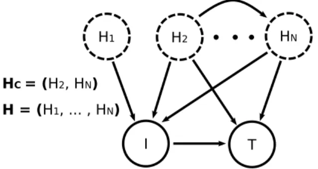
H1 H2

I T

HN

H = (H1, ... , HN) HC = (H2, HN)

Figure 2: A general model of visual causation. In our model each imageIis caused by a number of hidden non-visual variablesHi, which need not be independent. The

image itself is the only observed cause of a target behavior T. In addition, a (not necessarily proper) subset of the hid-den variables can be a cause of the target behavior. These confounders create visual “spurious correlates” of the be-havior inI.

of an image allows us to predict the value ofT. However, the predictive probability assigned to an image does not tell us the causaleffect of the image onT. For example, a barometer is widely taken to be an excellent predictor of the weather. But changing the barometer needle does not cause an improvement of the weather. It is not a (visual or otherwise) cause of the weather. In contrast, seeing a particular barometer reading may well be avisual causeof whether we pack an umbrella.

Our notion of a visual cause depends on the ability to ma-nipulate the image.

Definition 2(Visual Manipulation). Avisual manipulation is the operationman(I=i)that changes (the pixels of) the image to imagei ∈ I, while not affecting any other vari-ables (such asHorT). That is, the manipulated probabil-ity distribution of the generative model in Eq.(1)is given byP(T |man(I=i)) =P

HcP(T |I=i,Hc)P(Hc). The manipulation changes the values of the image pixels, but does not change the underlying “world”, represented in our model by theHi that generated the image. Formally,

the manipulation is similar to thedo-operator for standard causal models. However, we here reserve thedo-operation for interventions on causalmacro-variables, such as the vi-sual cause ofT. We discuss the distinction in more detail below.

We can now define thecausal partitionof the image space (with respect to the target behaviorT) as:

Definition 3(Causal Partition, Causal Class). The causal partitionΠc(T,I)of the setIw.r.t. behaviorTis the

par-tition induced by the equivalence relation∼defined onI

such thati∼jif and only ifP(T |man(I=i)) =P(T | man(I =j))fori, j ∈ I. When the image space and the target behavior are clear from the context, we will indicate the causal partition byΠc. A cell of a causal partition is

called acausal class.

The underlying idea is that images are considered causally equivalent with respect toT if they have the same causal effect onT. Given the causal partition of the image space, we can now define the visual cause ofT:

Definition 4(Visual Cause). Thevisual causeCof a target behaviorT is a random variable whose value stands in a bijective relation to the causal class ofI.

The visual cause is thus a function over I, whose values correspond to the post-manipulation distributions C(i) =

P(T | man(I = i)). We will writeC(i) = cto indicate that the causal class of imagei∈ Iisc, or in other words, that in imagei, the visual causeC takes valuec. Know-ingC allows us to predict the effects of a visual manipu-lationP(T | man(I =i)), as long as we have estimated P(T | man(I = i∗_k)) for one representativei∗_k of each causal classk.

2.3 THE CAUSAL COARSENING THEOREM Our main theorem relates the causal and observational par-titions for a givenI andT. It turns out that in general the causal partition is a coarsening of the observational parti-tion. That is, the causal partition aligns with the observa-tional partition, but the observaobserva-tional partition may subdi-vide some of the causal classes.

Theorem 5(Causal Coarsening). Among all the genera-tive distributions of the form shown in Fig. 2 which in-duce a given observational partitionΠo, almost all induce

a causal partitionΠcthat is a coarsening of theΠo.

Throughout this article, we use “almost all” to mean “all except for a subset of Lebesgue measure zero”. Fig. 3 il-lustrates the relation between the causal and the observa-tional partition implied by the theorem. We note that the measure-zero subset whereΠC does not coarsenΠO can

indeed be non-empty. We provide such counter-examples in Appendix 7.

We prove the CCT in Appendix 6 using a technique that extends that of Meek (1995): We show that (1) restricting the space of all the possibleP(T, H, I)to only the distribu-tions compatible with a fixed observational partition puts a linear constraint on the distribution space; (2) requiring that the CCT be false puts a non-trivial polynomial constraint on this subspace, and finally, (3) it follows that the theo-rem holds for almost all distributions that agree with the given observational partition. The proof strategy indicates a close connection between the CCT and the faithfulness assumption (Spirtes et al., 2000).

Two points are worth noting here: First, the CCT is in-teresting inasmuch as the visual causes of a behavior do not contain all the information in the image that predict the behavior. Such information, though not itself a cause of

(5)

P(T=0 | do{ }) = .17 P(T=0 | do{ }) = .83 P(T=0 | ) = .33 P(T=0 | ) = .66 P(T=0 | ) = 0 P(T=0 | ) = 1

Figure 3: The Causal Coarsening Theorem. The observa-tional probabilities of T given I (gray frame) induce an observational partition on the space of all the images (left, observational partition in gray). The causal probabilities (red frame) induce a causal partition, indicated on the left in red. The CCT allows us to expect that the causal partition is a coarsening of the observational partition. The observa-tional and causal probabilities correspond to the generative model shown in Fig. 1.

the behavior, can be informative about the state of other non-visual causes of the target behavior. Second, the CCT allows us to take any classification problem in which the data is divided into observational classes, and assume that the causal labels do not change within each observational class. This will help us develop efficient causal inference algorithms in Section 3.

2.4 VISUAL CAUSES IN A CAUSAL MODEL CONSISTING OF MACRO-VARIABLES We can now simplify our generative model by omitting all the information inIunrelated to behaviorT. Assume that the observational partitionΠT

o refines the causal

parti-tionΠT

c. Each of the causal classesc1,· · · , cK delineates

a region in the image spaceI such that all the images be-longing to that region induce the same P(T | man(I)). Each of those regions—say, the k-th one—can be further partitioned into sub-regions sk

1,· · ·, skMk such that all the images in the m-th sub-region of the k-th causal region in-duce the same observational probabilityP(T |I). By as-sumption, the observational partition has a finite number of classes, and we can arbitrarily order the observational classes within each causal class. Once such an ordering is fixed, we can assign an integerm ∈ {1,2,· · ·, Mk}to

each imageibelonging to the k-th causal class such thati belongs to the m-th observational class among theMk

ob-servational classes contained in ck. By construction, this

integer explains all the variation of the observational class within a given causal class. This suggests the following definition:

Definition 6 (Spurious Correlate). The spurious correlate S is a discrete random variable whose value differentiates between the observational classes contained in any causal

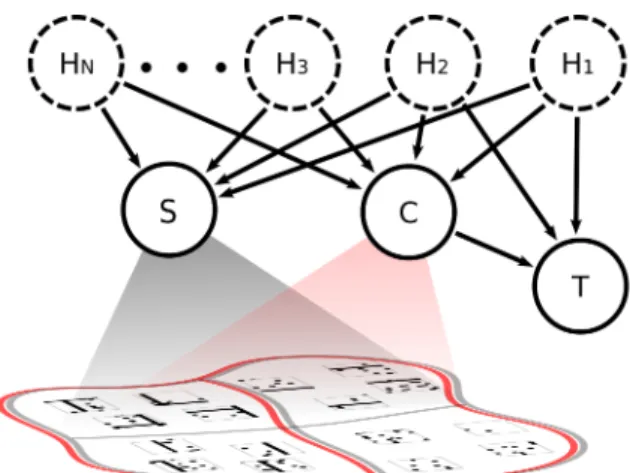
Figure 4: A macro-variable model of visual causation. Us-ing our theory of visual causation we can aggregate the in-formation present in visual micro-variables (image pixels) into the visual causeCand spurious correlateS. According to Theorem 7,CandScontain all the information aboutT available inI.

class.

The spurious correlate is a well-defined function on I, whose value ranges between1andmaxkMk. LikeC, the

spurious correlateS is a macro-variable constructed from the pixels that make up the image. CandS together con-tain all and only the visual information inIrelevant toT, but onlyCcontains the causal information:

Theorem 7(Complete Macro-variable Description). The following two statements hold for C and S as defined above:

1. P(T |I) =P(T |C, S).

2. Any other variableXsuch thatP(T |I) =P(T |X)

has Shannon entropyH(X)≥H(C, S).

We prove the theorem in Appendix 8. It guarantees thatC andSconstitute the smallest-entropy macro-variables that encompass all the information about the relationship be-tweenTandI. Fig. 4 shows the relationship betweenC, S andT, the image spaceIand the observational and causal partitions schematically. Cis now a cause of T,S corre-lates with T due to the unobserved common causesHC,

and any information irrelevant toTis pushed into the inde-pendent noise variables (commonly not shown in graphical representations of structural equation models).3

The macro-variable model lends itself to the standard treatment of causal graphical models described in Pearl (2009). We can define interventions on the causal vari-ables{C, S, T}using the standarddo-operation. Thedo -operator only sets the value of the intervened variable to

3

We note thatC may retain predictive information aboutT that is not causal, i.e. it is not the case that all spurious correlations can be accounted for inS. See Appendix 9 for an example.

(6)

the desired value, making it independent of its causes, but it does not (directly) affect the other variables in the sys-tem or the relationships between them (see themodularity assumptionin Pearl (2009)). However, unlike the standard case where causal variables are separated in location (e.g. smokingandlung cancer), the causal variables in an image may involve the same pixels:Cmay be the average bright-ness of the image, whereasSmay indicate the presence or absence of particular shapes in the image. An intervention on a causal variable using thedo-operator thus requires that the underlying manipulation of the image respects the state of the other causal variables:

Definition 8 (Causal Intervention on Macro-variables). Given the set of macro-variables{C, S}that take on values

{c, s}for an imagei∈ I, an interventiondo(C =c0)on the macro-variable C is given by the manipulation of the imageman(I =i0)such thatC(i0) = c0 andS(i0) = s. The interventiondo(S =s0)is defined analogously as the change of the underlying image that keeps the value ofC constant.

In some cases it can be impossible to manipulateCto a de-sired value without changingS. We do not take this to be a problem special to our case. In fact, in the standard macro-variable setting of causal analysis we would expect inter-ventions to be much more restricted by physical constraints than we are with our interventions in the image space.

3

CAUSAL FEATURE LEARNING:

INFERENCE ALGORITHMS

Given the theoretical specification of the concepts of in-terest in the previous section, we can now develop algo-rithms to learnC, the visual cause of a behavior. In addi-tion, knowledge ofCwill allow us to specify a manipula-tor function: a function that, given any image, can return a maximally similar image with the desired causal effect. Definition 9(Manipulator Function). LetCbe the causal variable of T and d a metric on I. The manipulator function ofC is a functionMC:I × C → I such that

MC(i, k) = arg minˆı∈C−1₍_k₎d(i,ˆı)for anyi∈ I, k∈ C.

In cased(i, .)has multiple minima, we group them together into one equivalence class and leave the choice of the rep-resentative to the manipulator function.

The manipulator searches for an image closest toIamong all the images with the desired causal effectk. The mean-ing of “closest” depends on the metricdand is discussed further in Section 3.2 below. Note that the manipulator function can find candidates for the image manipulation underlying the desired causal manipulationdo(C=c),but it does not check whether other variables in the system (in particular, the spurious correlate) remain in fact unchanged. Using the closest possible image with desired causal effect is a heuristic approach to fulfilling that requirement.

Algorithm 1:Causal Predictor Training input :Dobs={(i1, p1=p(T |i1)),· · ·,

(iN, pN =p(T |iN)}– observational data

P ={P1,· · ·, PM}– the set of

observatio-nal classes (so that∀k, pk ∈ P,1≤k≤N)

Train– a neural net training algorithm output:C: I →[0,1]– the causal variable

1 Pick{ik1,· · · , ikM} ⊂ {i1,· · · , iN}s.t.pkm =Pm; 2 EstimateCˆm←P(T |man(I=ikm))for eachm; 3 For allkletCˆ(ik)←Cˆmifpk=Pm;

4 Dcsl← {(i1,Cˆ(i1)),· · ·,(iN,Cˆ(iN))};

5 C←Train(Dcsl);

There are several reasons why we might want such a ma-nipulator function:

• If our goal is to perform causal manipulations on im-ages, the manipulator function offers an automated so-lution.

• A manipulator that uses a givenC and produces im-ages with the desired causal effect provides strong evi-dence thatCis indeed the visual cause of the behavior.

• Using the manipulator function we can enrich our dataset with new datapoints, in hope of achieving bet-ter generalization on both the causal and predictive learning tasks.

The problem of visual causal feature learning can now be posed as follows: Given an image spaceI and a metricd, learnC—the visual cause ofT—and the manipulatorMC.

3.1 CAUSAL EFFECT PREDICTION

A standard machine learning approach to learning the rela-tion between I andT would be to take an observational dataset Dobs = {(ik, P(T | ik))}k=1,···,N and learn a

predictorf whose training performance guarantees a low test error (so that f(i∗) ≈ P(T | i∗) for a test image i∗). In causal feature learning, low test error on observa-tional data is insufficient; it is entirely possible thatD con-tains spurious information useful in predicting test labels which is nevertheless not causal. That is, the prediction may be highly accurate for observational data, but com-pletely inaccurate for a prediction of the effect of a manip-ulation of the image (recall the barometer example). How-ever, we can use the CCT to obtain a causal dataset from the observational data, and then train a predictor on that dataset. Algorithm 1 uses this strategy to learn a func-tion C that, presented with any image i ∈ I, returns C(i) ≈P(T | man(I = i)). We use a fixed neural net-work architecture to learnC, but any differentiable hypoth-esis class could be susbtituted instead. Differentiability of Cis necessary in Section 3.2 in order to learn the manipu-lator function.

(7)

In Step 1 the algorithm picks a representative member of each observational class. The CCT tells us that the causal partition coarsens the observational one. That is, in principle (ignoring sampling issues) it is sufficient to estimate Cˆm = P(T | man(I = ikm)) for just one image in an observational class m in order to know that P(T |man(I=i)) = ˆCmfor any otheriin the same

ob-servational class. The choice of the experimental method of estimating the causal class in Step 2 is left to the user and depends on the behaving agent and the behavior in question. If, for example, T represents whether the spik-ing rate of a recorded neuron is above a fixed threshold, estimatingP(T |man(I=i))could consist of recording the neuron’s response toiin a laboratory setting multiple times, and then calculating the probability of spiking from the finite sample. The causal dataset created in Step 4 con-sists of the observational inputs and their causal classes. The causal dataset is acquired throughO(N)experiments, whereN is the number of observational classes. The fi-nal step of the algorithm trains a neural network that pre-dicts the causal labels on unseen images. The choice of the method of training is again left to the user.

3.2 CAUSAL FEATURE MANIPULATION

Once we have learnedCwe can use the causal neural net-work to create synthetic examples of images as similar as possible to the originals, but with a different causal label. The meaning of “as similar as possible” depends on the image metricd(see Definition 9). The choice ofdis task-specific and crucial to the quality of the manipulations. In our experiments, we use a metric induced by anL2norm. Alternatives include other Lp-induced metrics, distances

in implicit feature spaces induced by image kernels (Har-chaoui and Bach, 2007; Grauman and Darrell, 2007; Bosch et al., 2007; Vishwanathan, 2010) and distances in learned representation spaces (Bengio et al., 2013).

Algorithm 2 proposes one way to learn the manipulator function using a simple manipulation procedure that ap-proximates the requirements of Definition 9 up to local minima. The algorithm, inspired by the active learning techniques of uncertainty sampling (Lewis and Gale, 1994) and density weighing (Settles and Craven, 2008), starts off by training a causal neural network in Step 2. If only ob-servational data is available, this can be achieved using Al-gorithm 1. Next, it randomly chooses a set of images to be manipulated, and their target post-manipulation causal la-bels. The loop that starts in Step 6 then takes each of those images and searches for the image that, among the images with the same desired causal class, is closest to the original image. Note that the causal class boundaries are defined by the current causal neural netC. SinceCis in general a highly nonlinear function and it can be hard to find its in-verse sets, we use an approximate solution. The algorithm thus finds the minimum of a weighted sum of|C(j)−ˆcl,k|

Algorithm 2:Manipulator Function Learning input :d: I × I →R+– a metric on the image

space

Dcsl={(i1, c1),· · ·(iN, cN)}– causal data

C={C1,· · · , CM}– the set of causal

classes (so that∀ici∈ C)

Train– a neural net training algorithm nIters– number of experiment iterations Q– number of queries per iteration α– manipulation tuning parameter

A:I → C– an oracle forP(T |do(I))

output:MC:I × C → I– the manipulator function

1 forl←1tonItersdo 2 C←Train(Dcsl);

3 Choose manipulation starting points

{il,1,· · ·, il,Q}at random fromDcsl;

4 Choose manipulation targets{ˆcl,1,· · ·,ˆcl,Q}

such thatˆcl,k6=cl,k; 5 fork←1toQdo 6 ˆıl,k←argmin j∈I (1−α)|C(j)−cˆl,k| +α d(j, il,k); 7 end 8 Dcsl← Dcsl∪ {(ˆıl,1,A(ˆıl,1)),· · ·, (ˆıl,Q,A(ˆıl,Q))}; 9 end

(the difference of the output imagej’s label and the desired labelˆcl,k) andd(il,k, j)(the distance of the output imagej

from the original imageil,k).

At each iteration, the algorithm performsQmanipulations and the same number of causal queries to the agent, which result in new datapoints(ˆıl,1, A(ˆıl,1)),· · ·,(ˆıl,Q, A(ˆıl,Q)).

It is natural to claim that the manipulator performs well if A(ˆıl,k) ≈ˆcl,kfor manyk, which means the target causal

labels agree with the true causal labels. We thus define the manipulation errorof thelth iterationMErrlas

MErrl= 1 Q Q X k=1 |A(ˆıl,k)−ˆcl,k|. (2)

While it is important that our manipulations are accurate, we also want them to be minimal. Another measure of in-terest is thus theaverage manipulation distance

MDistl= 1 Q Q X k=1 d(Il,k,ˆıl,k). (3)

A natural variant of Algorithm 2 is to setnItersto a large integer and break the loop when one or both of these per-formance criteria reaches a desired value.

(8)

4

EXPERIMENTS

In order to illustrate the concepts presented in this article we perform two causal feature learning experiments. The first experiment, called GRATING, uses observational and causal data generated by the model from Section 1.2. The GRATING experiment confirms that our system can learn the ground truth cause and ignore the spurious correlates of a behavior. The second experiment,MNIST, uses images of hand-written digits (LeCun et al., 1998) to exemplify the use of the manipulator function on slightly more realistic data: in this example, we transform an image into a maxi-mally similar image with another class label.

We chose problems that are simple from the computer vi-sion point of view. Our goal is to develop the theory of visual causal feature learning and show that it has feasible algorithmic solutions; we are at this point not engineering advanced computer vision systems.

4.1 THEGRATINGEXPERIMENT

In this experiment we generate data using the model of Fig. 1, with two minor differences: H1 andH2 only in-duce one v-bar or h-bar in the image and we restrict our observational dataset to images with only about 3% of the pixels filled with random noise (see Fig. 5). Both restric-tions increase the clarity of presentation. We use Algo-rithms 1 and 2 (with minor modifications imposed by the binary nature of the images) to learn the visual cause of behaviorT.

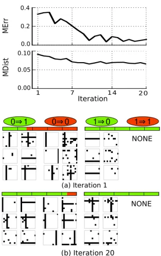
Figure 5 (top) shows the progress of the training process. The first step (not shown in the figure) uses the CCT to learn the causal labels on the observational data. We then train a simple neural network (a fully connected network with one hidden layer of 100 units) on this data. The same network is used on Iteration 1 to create new manipulated exemplars. We then follow Algorithm 2 to train the manip-ulator iteratively. Fig. 5 (bottom) illustrates the difference between the manipulator on Iteration 1 (which fails almost 40% of the time) and Iteration 20, where the error is about 6%. Each column shows example manipulations of a par-ticular kind. Columns with green labels indicate successful manipulations of which there are two kinds: switching the causal variable on (0⇒1, “adding the h-bar”), or switch-ing it off (1 ⇒ 0, “removing the h-bar”). Red-labeled columns show cases in which the manipulator failed to in-fluence the cause: That is, each red column shows an origi-nal image and its manipulated version which the manipula-tor believes should cause a change inT, but which does not induce such change. The red/green horizontal bars show the percentage of success/error for each manipulation di-rection. Fig. 5 (bottom, a) shows that after training on the causally-coarsened observational dataset, the manipulator fails about 40% of the time. In Fig. 5 (b), after twenty ma-nipulator learning iterations, only six manipulations out of

M D is t 1 7 14 20 M Er r 1 7 14

0

⇒

1

0

⇒

0

1

⇒

0

1

⇒

1

(a) Iteration 1 NONE NONE (b) Iteration 10 Iteration 0.0 0.2 0.4 0.10 0.05 0.00 20

Figure 5: Manipulator learning for GRATING. Top. The plots show the progress of our manipulator function learn-ing algorithm over ten iterations of experiments for the GRATING problem. The manipulation error decreases quickly with progressing iterations, whereas the manipu-lation distance stays close to constant. Bottom. Original and manipulatedGRATINGimages. See text for the details. a hundred are unsuccessful. Furthermore, the causally ir-relevant image pixels are also much better preserved than at iteration 1. The fully-trained manipulator correctly learned to manipulate the presence of the h-bar to cause changes in T, and ignores the v-bar that is strongly correlated with the behavior but does not cause it.

4.2 THEMNIST ON MTURKEXPERIMENT In this experiment we start with the MNIST dataset of handwritten digits. In our terminology, this – as well as any standard vision dataset – is already causal data: the labels are assigned in an experimental setting, not “in nature”. Consider the following binary human behavior: T = 1

if a human observer answers affirmatively to the question “Does this image contain the digit ‘7’?”, whileT = 0if the observer judges that the image does not contain the digit ‘7’. For simplicity we will assume that for any image

(9)

ei-Starting Digit Target Class 0 1 2 3 4 5 6 7 8 9 Iteration 0.0 0.5 1.0 0.0 0.05 0.1 1 2 3 4 MEr r MDis t 1 2 3 4 5 1 2 3 4 5

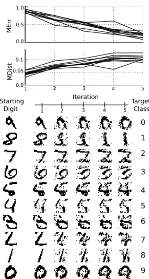
Figure 6: Manipulator Learning for MNIST ON MTURK. Top. In contrast to the GRATING experiment, here the manipulation distance grows as the manipulation error de-creases. This is because a successful manipulator needs to change significant parts of each image (such as continuous strokes).Bottom.Visualization of manipulator training on randomly selected (not cherry-picked)MNIST digits. See text for the details.

therP(T= 1|man(I)) = 0orP(T = 1|man(I)) = 1. Our task is to learn the manipulator function that will take any image and modify it minimally such that it will become a ‘7’ if it was not before, or will stop resembling a ‘7’ if it did originally.

We conduct the manipulator training separately for all the tenMNISTdigits using human annotators on Amazon Me-chanical Turk. The exact training procedure is described in Appendix 10. Fig. 6 (top) shows training progress. As in Fig. 5, the manipulation error decreases with train-ing. Fig. 6 (bottom) visualizes the manipulator training progress. In the first row we see a randomly chosen MNIST “9” being manipulated to resemble a “0”, pushed through successive “0-vs-all” manipulators trained at itera-tions 0, 1, ..., 5 (iteration 1 shows what the neural net takes to be the closest manipulation to change the “9” to a “0”

purely on the basis of the non-manipulated data). Further rows perform similar experiments for the other digits. The plots show how successive manipulators progressively re-move the original digits’ features and add target class fea-tures to the image.

5

DISCUSSION

We provide a link between causal reasoning and neu-ral network models that have recently enjoyed tremen-dous success in the fields of machine learning and com-puter vision (LeCun et al., 1998; Russakovsky et al., 2014). Despite very encouraging results in image classi-fication (Krizhevsky et al., 2012), object detection (Dollar et al., 2012) and fine-grained classification (Branson et al., 2014; Zhang et al., 2014), some researchers have found that visual neural networks can be easily fooled using adver-sarial examples (Szegedy et al., 2014; Goodfellow et al., 2014). The learning procedure for our manipulator func-tion could be viewed as an attempt to train a classifier that is robust against such examples. The procedure uses causal reasoning to improve on the boundaries of a standard, cor-relational classifier (Fig. 5 and 6 show the improvement). However, the ultimate purpose of a causal manipulator net-work is to extract truly causal features from data and au-tomatically perform causal manipulations based on those features.

A second contribution concerns the field of causal discov-ery. Modern causal discovery algorithms presuppose that the set of causal variables is well-defined and meaning-ful. What exactly this presupposition entails is unclear, but there are clear counter-examples: xand2xcannot be two distinct causal variables. There are also well understood problems when causal variables are aggregates of other variables (Chu et al., 2003; Spirtes and Scheines, 2004). We provide an account of how causal macro-variables can supervene on micro-variables.

This article is an attempt to clarify how one may construct a set of well-defined causal macro-variables that function as basic relata in a causal graphical model. This step strikes us as essential if causal methodology is to be successful in areas where we do not have clearly delineated candidate causes or where causes supervene on micro-variables, such as in climate science and neuroscience, economics and—in our specific case—vision.

Acknowledgements

KC’s work was funded by the Qualcomm Innovation Fel-lowship 2014. KC’s and PP’s work was supported by the ONR MURI grant N00014-10-1-0933. FE would like to thank Cosma Shalizi for pointers to many relevant results this paper builds on.

(10)

6

APPENDIX: PROOF OF THE CAUSAL

COARSENING THEOREM

Before we prove the Causal Coarsening Theorem, we prove its less general version in order to split the rather complex proof of CCT into two parts. This Auxiliary Theorem can be proven using simpler techniques, however here we de-liberately use techniques that transfer directly to the proof of the CCT.

Auxiliary Theorem Among all the generative models of the form discussed in Fig. 2 (in the main text), the subset of distributions P(T, H, I)for which the causal partition is not a coarsening (proper or improper) of the observational partition is Lebesgue measure zero.

Proof. Our proof is inspired by a proof used by Meek (1995) to prove that almost all distributions compatible with a given causal graph are faithful. The proof strat-egy is thus first to express the proposition that for a given distribution, the observational partition does not refine the causal partition as a polynomial equation on the space of all distributions compatible with the model. We then show that this polynomial equation is not trivial, i.e. there is at least one distribution that is not its root. By a simple al-gebraic lemma, this will prove the theorem. We extend Meek’s proof technique in our usage of Fubini’s Theorem for the Lebesgue integral. It allows us to “split” the poly-nomial constraint into multiple different constraints along several of the distribution parameters. This allows for ad-ditional flexibility in creating useful assumptions (in our proof, the assumption that the datapoints have well-defined causal classes, but the observational class can still vary freely).

Assume thatT is binary andH = (H1,· · ·, HM),I are

discrete variables (say|Hi|=Ki,|I|=N, thoughN can

be very large. We will use the notationK_,K1×· · ·×KM

for simplicity later on). The discreteness assumption is not crucial, but will simplify the reasoning. We can factorize the joint as P(T, H, I) = P(T | H, I)P(I | H)P(H). P(T |H, I)can be parametrized by|H1| × · · · × |HM| ×

|I|=K×Nparameters,P(I |H)by(N−1)×K pa-rameters, andP(H)by anotherKparameters, all of which are independent. Call the parameters, respectively,

αh,i,P(T = 0|H =h, I=i)

βi,h,P(I=i|H =h)

γh,P(H =h)

We will denote parameter vectors as α= (αh1,i1,· · ·, αhK,iN)∈R K×N β = (βi1,h1,· · · , βiN−1,hK)∈R (N−1)×K γ= (γh1,· · · , γhK)∈R K_,

where the indices are arranged in lexicographical order. This creates a one-to-one correspondence of each possi-ble joint distributionP(T, H, I)with a point(α, β, γ) ∈ P[α, β, γ] ⊂ RK

3_×_N_×₍_N₋₁₎

, where P[α, β, γ] is the K3_×_N_×₍_N ₋₁₎_{-dimensional simplex of multinomial} distributions.

To proceed with the proof, we first pick any point in the P(T |H, I)×P(H)space: that is, we fix the values ofα andγ. The only free parameters are nowβi,hfor all values

ofi, h; varying these values creates a subset of the space of all the distributions which we will call

P[β;α, γ] ={(α, β, γ) | β∈[0,1](N−1)×K}. P[β;α, γ] is a subset of P[α, β, γ] isometric to the

[0,1](N−1)×K_{-dimensional simplex of multinomials. We}

will use the term P[β;α, γ] to refer both the subset of P[α, β, γ]and the lower-dimensional simplex it is isomet-ric to, remembering that the latter comes equipped with the Lebesgue measure onR(N−1)×K.

Now we are ready to show that the subset of P[β;α, γ]

which does not satisfy the Causal Coarsening constraint is of measure zero with respect to the Lebesgue measure. To see this, first note that sinceαandγ are fixed, each im-ageihas a well-defined causal classC(i) = P

hαh,iγh.

The Causal Coarsening constraint says “For every pair of images i, j such thatP(T | i) = P(T | j)it holds that C(i) =C(j).” The subset ofP[β;α, γ]of all distributions that do not satisfy the constraint consists of theP(T, H, I)

for which for somei, jit holds that

P(T = 0|i) =P(T = 0|j) and C(i)6=C(j). Take any pair i, jfor whichC(i) 6= C(j)(if such a pair does not exist, then the Causal Coarsening constraint holds for all the distributions inP[β;α, γ]). We can write

Since the same equation applies toP(T = 0|j), the con-straintP(T |i) =P(T |j)can be rewritten

(11)

which we can rewrite in terms of the independent param-eters (after definingα0,h,i =αh,iandα1,h,i = 1−αh,i)

and further simplify as

  X t∈{0,1} X h αt,h,jγhβj,h   X h α0,h,iγhβi,h− −   X t∈{0,1} X h αt,h,iγhβi,h   X h α0,h,jγhβj,h = 0 ⇐⇒ X h α1,h,jγhβj,h ! X h α0,h,iγhβi,h− − X h α1,h,iγhβi,h ! X h α0,h,jγhβj,h = 0 ⇐⇒ X h (1−αh,j)γhβj,h ! X h αh,iγhβi,h− − X h (1−αh,i)γhβi,h ! X h αh,jγhβj,h = 0 ⇐⇒ X h γhβj,h ! X h αh,iγhβi,h− − X h γhβi,h ! X h αh,jγhβj,h = 0, (4)

which is a polynomial constraint on P[β;α, γ](note that to keep the notation manageable, we have omitted the de-pendent term1−P

hγhfrom the equations). By a simple

algebraic lemma (proven by Okamoto, 1973), if the above constraint is not trivial (that is, if there existsβ for which the constraint does not hold), the subset ofP[β;α, γ]on which it holds is measure zero.

To see that Eq. (4) does not always hold, note that if forany h∗ we setβi,h∗ = 1(and thusβ_i,h = 0for anyh6= h∗) andβj,h∗= 1, the equation reduces to

(γh∗)2(α_h

i,i−αhj,h) = 0.

Thus if Eq. (4) was trivially true, we would have αh,i =

αh,j orγh = 0for allh. However, this impliesC(i) =

C(j), which contradicts our assumption.

We have now shown that the subset of P[β;α, γ] which consists of distributions for whichP(T | i) = P(T | j)

(even though C(i) 6= C(j)) is Lebesgue measure zero. Since there are only finitely many pairs of imagesi, j for whichC(i) 6= C(j), the subset ofP[β;α, γ] of distribu-tions which violate the Causal Coarsening constraint is also

Lebesgue measure zero. The remainder of the proof is a di-rect application of Fubini’s theorem.

For eachα, γ, call the (measure zero) subset ofP[β;α, γ]

that violates the Causal Coarsening constraintz[α, γ]. Let Z =∪α,γz[α, γ]⊂P[α, β, γ]be the set of all the joint

dis-tributions which violate the Causal Coarsening constraint. We want to prove thatµ(Z) = 0, whereµis the Lebesgue measure. To show this, we will use the indicator function

ˆ

z(α, β, γ) =

1 ifβ∈z[α, γ],

0 otherwise.

By the basic properties of positive measures we have

µ(Z) =

Z

P[α,β,γ]

ˆ

z dµ.

It is a standard application of Fubini’s Theorem for the Lebesgue integral to show that the integral in question equals zero. For simplicity of notation, let

A=RK×N B=_RN×K G=RK. We have Z P[α,β,γ] ˆ z dµ= Z A×B×G ˆ z(α, β, γ)d(α, β, γ) = Z A×G Z B ˆ z(α, β, γ)d(β)d(α, γ) = Z A×G µ(z[α, γ])d(α, γ) (5) = Z A×G 0d(α, γ) = 0.

Equation (5) follows aszˆrestricted toP[β;α, γ]is the in-dicator function ofz[α, γ].

This completes the proof that Z, the set of joint distribu-tions over T, H andI that violate the Causal Coarsening constraint, is measure zero.

We are now ready to prove the main theorem.

Theorem (Causal Coarsening Theorem) Among all the generative models of the form discussed in Fig. 2 (in the main text) that have distributions P(T,H, I) that induce some given observational partition Πo,almost all

(12)

Proof. Any variables that appear in this proof without def-inition are defined in the proof of the Auxiliary Theorem. We take the sameα, β, γ parametrization of distributions. Fixing an observational partition means fixing a set of ob-servational constraints (OCs)

P(T |i1₁) =· · ·=P(T |i1_N

1),

.. .

P(T |iL1) =· · ·=P(T |iLNK),

where1≤L≤N is the number of observational classes. SinceP(T, H, I) =P(H |T, I)P(T |I)P(I),P(T |i)

is an independent parameter in the unrestrictedP(T, H, I), and the OCs reduce the number of independent parameters of the joint by PL

l=1(Nl −1). We want to express this

parameter-space reduction in terms of theα, β andγ pa-rameterization and then apply the proof of the Auxiliary Theorem. To do this, for each observational classl, choose a representative imageˆıl_{such that}

P(T |il_m) =P(T |ˆıl) ∀m∈1···Nk. Then for eachil

m6= ˆılit holds that P(T, il_m) =P(T |ˆıl)P(il_m) or X h P(T, h, il_m) =P(T |ˆıl)X h P(h, il_m). Picking an arbitraryh0, we can separate the left-hand side as P(T, h0, il_m) =P(T |ˆıl)X h P(h, il_m)−X h6=h0 P(T, h, il_m).

Finally, this equation can be rewritten in terms ofα, βand γas αh0,iβi,h0γh0 =P(T |ˆı l₎X h βh,il mγh− X h6=h0 αh,il mβilmγh, or αh0,i= P(T |ˆıl₎P hβh,il mγh− P h6=h0αh,ilmβilmγh βi,h0γh0 for anyil

m 6= ˆıl. There are precisely

PL

l=1(Nl−1)such

equations, altogether equivalent to the observational con-straints. Thus we can express anyP(T, H, I)distribution that is consistent with a given observational partition in terms of the full range of β andγ parameters, and a re-stricted number of independentαparameters. The rest of the proof now follows similarily to the proof of the Auxil-iary Theorem and shows that within this restricted param-eter space, the paramparam-eters for which the (fixed) observa-tional partition is not a refinement of the causal partition is measure zero.

7

APPENDIX: CCT EXAMPLES AND

COUNTER-EXAMPLES

In Fig. 7 we provide examples of three distributions over binary variablesH, T and three-valuedI. The first model induces a causal partition that is a proper coarsening of the observational partition, and thus agrees with the CCT. The second model induces an observational partition that is a proper coarsening of the causal partition – CCT im-plies that this is a measure-zero case and that, after fix-ing the observational partition, we had to carefully tweak the parameters to align the causal partition as it is. The third model induces causal and observational partitions that are incompatible – that is, neither is a coarsening of the other. This is also a measure-zero case. We provide a Tetrad (http://www.phil.cmu.edu/tetrad/) file that contains these three models at http://vision. caltech.edu/˜kchalupk/code.html. It can be used to verify our observational and causal partition com-putations.

8

APPENDIX: PROOF OF THE

COMPLETE MACRO-VARIABLE

DESCRIPTION THEOREM

Theorem (Complete Macro-variable Description) The following two statements hold forC and S as defined in the main text:

1. P(T |I) =P(T |C, S).

2. Any other variableXsuch thatP(T |I) =P(T |X)

has Shannon entropyH(X)≥H(C, S).

Proof. The first part follows by construction ofS. For the second part, note that by the CCT there is a bijective cor-respondence between the pairs of values(c, s)and the ob-servational probabilities P(T | I). Call this correspon-dence f, that is f(c, s) = P(T | c, s) and f−1₍_p_{) =}

(c, s s.t.P(T|c, s) = p). Further, defineg as the func-tion onX,withg:x7→P(T |x). But sinceP(T |X) =

P(T |I), we have(c, s) =f−1(g(x)). That is, the value of C andS is a function of the value ofX, and thus the entropy ofCandSis smaller than the entropy ofX.

9

APPENDIX: PREDICTIVE

NON-CAUSAL INFORMATION IN

CAUSAL VARIABLE

C

In some casesC retains predictive information that is not causal. Consider the following example: We have a causal graph consisting of three variables {I, T, H} where the causal relations areI → T andI ← H → T. All three variables are binary and we have a positive distribution over

(13)

I=2

I=1

I=0

P(H=0) = 0.4572 P(I=0|H=0) = 0.3426 P(I=1|H=0) = 0.1239 P(I=0|H=1) = 0.3255 P(I=1|H=1) = 0.5097 P(T=0|H=0, I=0) = 0.13 P(T=0|H=0, I=1) = 0.233 P(T=0|H=0, I=2) = 0.05 P(T=0|H=1, I=0) = 0.12 P(T=0|H=1, I=1) = 0.0332 P(T=0|H=1, I=2) = 0.1141

I=2

I=1

I=0

I=2

I=1

I=0

H

I

T

{0,1}

{0,1,2}

{0,1}

Figure 7: A graphical causal model and three faithful prob-ability tables. The first (from the top) table induces a causal partition (red) that is a coarsening of the observa-tional partition (gray) – specifically, as the figure shows, P(T|I = 0) 6= P(T|I = 1)butP(T|man(I = 0)) =

P(T|man(I= 1)). The second table induces an observa-tional partition that is a corasening of the causal partition. The last table induces a causal and an observational parti-tion such that neither is a coarsening of the other.

the variables. In the general case, distributions over this graph satisfy

1. P(T|do(I= 1))6=P(T|do(I= 0))

2. P(T|I= 1)6=P(T|I= 0), and importantly 3. P(T|I)6=P(T|do(I)).

If we view I as an image (which can either be all black or all white), T as the target behavior andH as a hidden confounder, analogous to the set-up in the main article, then the observational partition Πo has just two classes,

namely {1,0}. But in this case the observational parti-tion is the same as the causal partition: Πo = Πc. So

by our definition of a spurious correlate, S is a constant, since there are no further distinctions to be made within any of the causal classes. S would be omitted from any standard causal model. Nevertheless, we have in our model still thatP(T|C) 6= P(T|do(C)), i.e. the causal variable C still contains predictive information that is not causal. Given that there is by construction no other than the causal and the trivial partition in this example, it must be the case thatCretains predictive non-causal information. It follows that in our definitions ofCandS, it is not the case that the predictive non-causal components of an image can always be completely separated from the causal features.

10

APPENDIX:THE

MNIST ON MTURK

EXPERIMENT

For this experiment, we started off by training ten one-vs-all neural nets. We used cross-validation to choose among the following architectures: 100 hidden units (h.u.), 300 h.u. (one layer), 100-100 h.u (two layers), 300-300 h.u. (two layers). We used maxout (Goodfellow and Warde-Farley, 2013) activations (each of which computed the max of 5 linear functions). For training we used stochastic gra-dient descent in batches of 50 with 50% dropout (Hinton and Srivastava, 2012) on the hidden units, momentum ad-justment from 0.5 to 0.99 at iteration 100, learning rate de-caying from 0.1 to 0.0001 with exponential coefficient of 1/0.9998, no weight decay, and we enforced the maximum norm of a column of hidden units to 5. The training stopped after 1000 iterations and the iteration with best validation error was chosen. We used the Pylearn2 package (Goodfel-low and Warde-Farley, 2013) to train the networks. This initial training was done on 5000 training points and 1250 validation points (both of which come from the MNISTdataset) for each machine. The training points were chosen at random to include 2500 images of a specific digit class (that is, 2500 zeros for the first machine, 2500 ones for the second machine and so on), and 2500 images of random other digits for each machine. The validation sets were composed similarly. Each machine then used

(14)

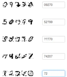
Algo-Figure 8: The Amazon Mechanical Turk interface we used to query online annotators. An annotator is shown five rows of five manipulated digit images, and is requested to type the digit labels (or ‘?’) into the input boxes. Each annotator goes through ten similar screens, annotating a total of 250 digits.

rithm 2 to transform 1000 images of digitsfrom its training setinto maximally similar images of the opposing class. We thus started off with ten manipulated datasets of 1000 images each. The first dataset contained images of zeros manipulated to be non-zeros, and all the other digits ma-nipulated to be zeros. The tenth dataset contained images of nines manipulated to be non-nines and the other digits manipulated to be nines. We then used Amazon Mechan-ical Turk to present all those images to human annotators, using the interface shown in Fig. 8. The images created by all the manipulator networks were mixed at random to-gether, so that each single annotator (annotating 250 im-ages in one task) would see some imim-ages created by each machine. Finally, each of the 10000 images was shown to five annotators; we used 5×40=200 annotators total on each iteration. The annotators labeled the images as either one of the ten digits, or the question mark ‘?’ if there was no recognizable digit in an image. The final label (“target digit” or “not target digit”) was chosen using majority of the annotators’ votes.

The annotated manipulated digits were then added to the datasets which their respective original images belonged to. We then proceeded to train the next iteration of neural net-work manipulators on the updated datasets, and so on until completion of the manipulator training.

References

Y. Bengio, A. Courville, and P. Vincent. Representation learning: A review and new perspectives. Pattern Anal-ysis and Machine Intelligence, 35(8):1798–1828, 2013. A. Bosch, A. Zisserman, and X. Munoz. Representing

shape with a spatial pyramid kernel. In6th ACM Interna-tional Conference on Image and Video Retrieval, pages 401–408, 2007.

S. Branson, G. Van Horn, and C. Wah. The Ignorant Led by the Blind: A Hybrid Human–Machine Vision System for Fine-Grained Categorization. International Journal of Computer Vision, 108(1-2):3–29, 2014.

T. Chu, C. Glymour, R. Scheines, and P. Spirtes. A statis-tical problem for inference to regulatory structure from associations of gene expression measurements with mi-croarrays. Bioinformatics, 19(9):1147–1152, 2003. P. Dollar, C. Wojek, B. Schiele, and P. Perona. Pedestrian

detection: An evaluation of the state of the art. IEEE Transactions on Pattern Analysis and Machine Intelli-gence, 34(4):743–761, 2012.

A. S. Fire and S. C. Zhu. Using causal induction in hu-mans to learn and infer causality from video. The An-nual Meeting of the Cognitive Science Society (CogSci), 2013a.

A. S. Fire and S. C. Zhu. Learning Perceptual Causality from Video. AAAI Workshop: Learning Rich Represen-tations from Low-Level Sensors, 2013b.

I. J. Goodfellow and D. Warde-Farley. Maxout networks. arXiv preprint arXiv:1302.4389, 2013.

I. J. Goodfellow, J. Shlens, and C. Szegedy. Explaining and Harnessing Adversarial Examples. arXiv preprint arXiv:1412.6572, 2014.

K. Grammer and R. Thornhill. Human (Homo sapiens) fa-cial attractiveness and sexual selection: The role of sym-metry and averageness. Journal of Comparative Psy-chology, 108(3):233–242, 1994.

K. Grauman and T. Darrell. The pyramid match kernel: Ef-ficient learning with sets of features.Journal of Machine Learning Research, 8:725–260, 2007.

I. Guyon, A. Elisseeff, and C. Aliferis. Causal feature se-lection. InComputational Methods of Feature Selection Data Mining and Knowledge Discovery Series, pages 63–85. Chapman and Hall/CRC, 2007.

Z. Harchaoui and F. Bach. Image classification with seg-mentation graph kernels. In IEEE Computer Society Conference on Computer Vision and Pattern Recogni-tion, pages 1–8, 2007.

G. E. Hinton and N. Srivastava. Improving neural networks by preventing co-adaptation of feature detectors. arXiv preprint arXiv:1207.0580, 2012.

(15)

E. P. Hoel, L. Albantakis, and G. Tononi. Quantifying causal emergence shows that macro can beat micro. Pro-ceedings of the National Academy of Sciences, 110(49): 19790–19795, 2013.

A. Krizhevsky, I. Sutskever, and G. E. Hinton. Ima-geNet Classification with Deep Convolutional Neural Networks. In F. Pereira, C. J. C. Burges, L. Bottou, and K. Q. Weinberger, editors,Advances in Neural Informa-tion Processing Systems 25, pages 1097–1105. 2012. Y. LeCun, L. Bottou, Y. Bengio, and P. Haffner.

Gradient-based learning applied to document recognition. Pro-ceedings of the IEEE, 86(11):2278–2324, 1998.

D. D. Lewis and W. A. Gale. A sequential algorithm for training text classifiers. InACM SIGIR Seventeenth Con-ference on Research and Development in Information Retrieval, pages 3–12, 1994.

C. Meek. Strong completeness and faithfulness in Bayesian networks. InEleventh Conference on Uncertainty in Ar-tificial Intelligence, pages 411–418, 1995.

M. Okamoto. Distinctness of the eigenvalues of a quadratic form in a multivariate sample. The Annals of Statistics, 1(4):763–765, 1973.

J. Pearl. Causality: Models, Reasoning and Inference. Cambridge University Press, 2009.

J. P. Pellet and A. Elisseeff. Using Markov blankets for causal structure learning. Journal of Machine Learning Research, 9:1295–1342, 2008.

O. Russakovsky, J. Deng, H. Su, J. Krause, S. Satheesh, S. Ma, Z. Huang, A. Karpathy, A. Khosla, M. Bernstein, A. C. Berg, and L. Fei-Fei. ImageNet large scale visual recognition challenge. arXiv preprint arXiv:1409.0575, 2014.

B. Settles and M. Craven. An analysis of active learning strategies for sequence labeling tasks. In Conference on Empirical Methods in Natural Langauge Processing, pages 1070–1079, 2008.

C. R. Shalizi. Causal architecture, complexity and self-organization in the time series and cellular automata. PhD thesis, University of Wisconsin at Madison, 2001. C. R. Shalizi and J. P. Crutchfield. Computational

me-chanics: Pattern and prediction, structure and simplicity. Journal of Statistical Physics, 104(3-4):817–879, 2001. P. Spirtes and R. Scheines. Causal inference of ambiguous

manipulations. Philosophy of Science, 71(5):833–845, 2004.

P. Spirtes, C. N. Glymour, and R. Scheines. Causation, prediction, and search. Massachusetts Institute of Tech-nology, 2nd ed. edition, 2000.

C. Szegedy, W. Zaremba, I. Sutskever, J. Bruna, D. Erhan, I. Goodfellow, and R. Fergus. Intriguing properties of neural networks. InInternational Conference on Learn-ing Representations, 2014.

S. V. N. Vishwanathan. Graph kernels.Journal of Machine Learning Research, 11:1201–1242, 2010.

N. Zhang, J. Donahue, R. Girshick, and T. Darrell. Part-based R-CNNs for fine-grained category detection. In ECCV 2014, pages 834–849, 2014.

http://vision.caltech.edu/˜kchalupk/code.html

(http://www.phil.cmu.edu/tetrad/