Design and Analysis of Two Highly Scalable Sparse Grid Combination Algorithms
Peter E. Strazdins
Research School of Computer Science Australian National University
Canberra, Australia [email protected]
Md Mohsin Ali
Research School of Computer Science Australian National University
Canberra, Australia [email protected]
Brendan Harding Mathematical Sciences Institute
Australian National University Canberra, Australia [email protected]
Abstract—Many petascale and exascale scientific simulations involve the time evolution of systems modelled as Partial Differential Equations (PDEs). The sparse grid combination technique (SGCT) is a cost-effective method for solve time-evolving PDEs, especially for higher-dimensional problems. It consists of evolving PDE over a set of grids of differing resolution in each dimension, and then combining the results to approximate the solution of the PDE on a grid of high resolution in all dimensions. It can also be extended to support algorithmic-based fault-tolerance, which is also important for computations at this scale.
In this paper, we present two new parallel algorithms for the SGCT that supports the full distributed memory parallelization over the dimensions of the component grids, as well as across the grids as well. The direct algorithm is so called because it directly implements a SGCT combination formula. We give details of the design and implementation of a ‘partial’ sparse grid data structure, which is needed for its efficient implementation. The second algorithm converts each component grid into their hierarchical surpluses, and then uses the direct algorithm on each of the hierarchical surpluses. The conversion to/from the hierarchical surpluses is also an important algorithm in its own right. It requires a technique called sub-griding in order to correctly deal with the combination of very small surpluses. An analysis of both indicates the direct algorithm minimizes the number of messages, whereas the hierarchical surplus minimizes memory consumption and offers a reduction in bandwidth by a factor of 1−2−d, wheredis the dimensionality of the SGCT. However, this is offset by its incomplete parallelism (70–80%) and a factor of2dload imbalance in practical scenarios. Our analysis also indicates both are suitable in a bandwidth-limited regime and that the direct algorithm is scalable with respect to d. Experimental results including the strong and weak scalability of the algorithms indicates that, for scenarios of practical inter-est, both are sufficiently scalable to support large-scale SGCT but the direct algorithm has generally better performance, at least by a factor of 2 in most cases. Hierarchical surplus formation is much less communication intensive, but shows less scalability with increasing core counts. Altering the layout of processes in the process grids and the mapping of processes affects the performance of the 2D SGCT by less than 10%, and affects even less the application part of an SGCT advection application.
Keywords
-high performance computing, parallel computing, PDE solvers, sparse grid combination technique, algorithm-based fault tolerance
I. INTRODUCTION
Large scale scientific simulations at the peta- and exascale are capable of making great advances in computational sci-ence. Usually, these involve the numerical solution ofPartial Differential Equations (PDEs). There are two main obsta-cles for scientific applications in order to reach this goal: achieving sufficient scalability, and ensuring their reliable completion. Both of these problems arise due the immense size, and hence number of components, of supercomputing systems at these scales. The latter problem arises due to the fact that these simulations are typically long-running, and that the failure rate of the system is proportional to the number of components.
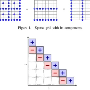
PDEs are normally solved on a regular grid. With uniform discretization across all its dimensions, the number of grid points increases exponentially with the increase of dimen-sionality. This behavior makes the high-dimensional PDE solver computationally expensive. In order to address this issue, the PDE can be solved on a grid with substantially fewer grid points than the regular full grid. These grids are calledsparse grids[1]. An example of a sparse grid is shown in Figure 1, where the sparse grid is represented as the union of smaller regular grids.
A numerical method called the Sparse Grid Combination Technique(SGCT) [2], [3] can be employed to approximate the solutions to PDEs on the sparse grid. Instead of solving the PDEs on a full grid, it solves them on severalanisotropic grids with substantially fewer grid points, called the sub-gridsor component grids, as shown in Figure 1. Solutions on these sub-grids are then linearly combined to approximate the solution on the sparse grid. The technique can be applied in principle to any PDE, but sufficient ‘smoothness’ of the solution is required for good accuracy.
An important technique associated with sparse grids is the formation ofhierarchical surpluses[4], [5] on regular grids. These facilitate error analysis over the various dimensions at various levels of resolution, and can be used to determine when refinement is required on adaptive grids [5].
As well as making high-dimensional PDEs tractable, employing the SGCT can result in computational efficiencies even for lower-dimensional problems [2], [3], [6], [7].
Fur-thermore, it inherently supports parallelism in the sense that component grids can be solved completely independently. The SGCT can also be extended to support algorithm-based fault-tolerance [8], [9], [7]. Upon detection of a fault, the SGCT can be applied in such a way that the component grids associated with the failed nodes are avoided. The lost data can be recovered by down-sampling from the combined (sparse) grid, and the computation can continue sustainably. The ability to repeatedly apply the SGCT over a computation is also useful in improving the accuracy of the sparse grid approximation in certain cases [6], [7].
Thus, there is an urgent need to have highly parallel SGCT and hierarchical surplus formation algorithms for where the component grids themselves are large and must be solved in parallel. The contributions of this paper are to (i) present two new algorithms for the SGCT which support fault-tolerance and are suitable for computations over a large number of cores and (ii) perform an analysis and detailed experimental evaluation of their performance. To the best of our knowledge, this is the first work that does so for a SGCT algorithm which supports distributed memory parallelism both across and within the component grids. The direct algorithm is furthermore highly general in terms of the process grid sizes used for the component grids (the hierarchical surplus algorithm requires these to be powers of 2). We also believe that we also give the first general distributed memory algorithm for the conversion of a grid to/from its hierarchical surpluses. We also are the first to discuss the concept of a partial sparse grid, and give the first implementation of a distributed sparse grid data structure. In order to do so, we introduce the concept of thesparse block distribution, which we believe is novel. Furthermore, we show how the hierarchical surpluses can be coalesced and scheduled, and show that the former is crucial for its efficiency. We give a deep analysis of the scaling behaviour of these algorithms, followed by a com-prehensive experimental evaluation, Finally, we expect that our approach to algorithm design and implementation using vector arithmetic and associated distribution mappings will be applicable to other communication-intensive algorithms over high dimensional spaces.
The paper is organized as follows. Section II describes the SGCT technique. Details of our implementation of a highly scalable SGCT algorithm are given in Section III, followed by an analysis in Section IV. Experimental results are given in Section V, related work is discussed in Section VI, and conclusions are given in Section VII.
II. THESPARSEGRIDCOMBINATIONTECHNIQUE
Consider the SGCT for the 2D case. Each component sub-gridGi, wherei= (ix, iy), is assumed to have(2ix+
1)×(2iy + 1) grid points with a grid spacing of h 1 = 2−ix andh
2= 2−iy in the x- and y-directions, respectively,
whereix, iy ≥0. If we consider a square domain, then the
133
J.W. Larson et al. / Procedia Computer Science 18 ( 2013 ) 130 – 139
= ∪ ∪
Fig. 1. A sparse grid with its components
3. MapReduce
MapReduce [5, 6] is a functional programming pattern popularized by Google, who have used it to compute page rank and inverted indices of the Internet. In broadest terms, the MapReduce programming model is the composition of oneMap()and oneReduce()–sometimes calledFold()–function, withReduce()operating on the outputs ofMap(). The discussion of sparse grid combination method in Section 4 and the 2D advection prototyped described in Section 5 employ the MapReduce pattern in this purely functional sense.
Google’s MapReduce programming model defines theMap()andReduce()functions as follows: theMap() transforms input data into a list of output<key,value>pairs; theReduce()phase transforms allvalues asso-ciated with a givenkeyinto a final result for thatkey. Mapoutputs are routed toReduceinputs by an inter-mediate sorting facility provided by the MapReduce framework. Data input into the framework, interinter-mediate <key,value>pairs, and the framework’s output are stored on a proprietary distributed file system (DFS). The <key,value>pairs are sorted, and grouped bykeyfor subsequent routing toReducenodes. Fault-tolerance is implemented using replication and task pools with reassignment. The Google MapReduce implementation is proprietary. Yahoo! have developed the open-source Hadoop implementation [20] that imitates the functionality and fault-tolerance of Google MapReduce. Hadoop is widely used in large-scale data analysis in the commercial and research communities. The rapid uptake of MapReduce has spawned other implementations, including one utilizing Python’s Pool class [21], and the message-passing-parallel MapReduce-MPI [22]. A review discussion of MapReduce implementations, advantages and disadvantages of the MapReduce programming model, and its variants and extensions is given by [23].
4. Sparse Grids and a Fault-tolerant Combination Technique
Sparse grids [24, 8] are computational grids that contain substantially fewer points than the usual regular isotropic grids. They are particularly suited to higher-dimensional problems as they are less affected by the curse of dimensionality. An example of a sparse grid is seen in Figure 1. The figure also shows that the sparse grid is represented as the union of regular grids. In the following discussion we only consider 2-dimensional grids. Any regular grid is assumed to have a grid spacing of 2−iin thexdirection and 2−jin theydirection. Following [25],
we call any union of regular grids a sparse grid.
The sparse grid combination technique [7, 8] approximates sparse grid solutions to PDEs by linear combina-tions of solucombina-tions on regular grids. Here we will consider a square domain in which the grid points of the regular gridsGi,jare{(2xi,
y
2i)|x=0,1, . . . ,2i,y=0,1, . . . ,2j}. For the example shown in Figure 1, five subgridsGi,jwith
2i+1 by 2j+1 grid points are required. These include in addition to the three constitutive gridsG
3,1,G1,3and G2,2the two intersection gridsG2,1andG1,2. The sparse grid itself may be defined using only the first three
GSG=G3,1∪G1,3∪G2,2
but for the combination technique approximation one requires the solutionsui,jon all the five gridsGi,jas the
approximation takes the form
uCT=u3,1+u1,3+u2,2−u2,1−u1,2.
The combination technique is a very general approach and has been used to obtain sparse grid approximations to problems for which solutions are available on regular grids. An example is the determination of eigenvalues,
Figure 1. Sparse grid with its components.
Figure 2. A depiction of SGCT combination coefficientsci, where+,−
and blank represent values of+1,−1and0, respectively. The combination
is of the form of Equation (2).
grid points of Gi are {(x 0 2ix, y0 2iy)|x 0 = 0,1,· · ·,2ix, y0 = 0,1,· · ·,2iy}.
In the more general case, the index space for the grids will be some finite set I ⊂ Nd. If u
i denotes the approximate solution of a PDE on Gi, the combination solution ucI generally takes the form
ucI =X
i∈I
ciui, (1)
where ci ∈ R are the combination coefficients. Clearly,
the accuracy of the combination technique approximation depends on the choice of the index space I of the sub-grids and their respective coefficients. For the 2D case, good choices of the coefficients are±1. For instance, in the clas-sical case, we have for levell the setI={(ix, iy)|ix, iy≥
0, l−1 ≤ ix+iy ≤ l} and the combination coefficients are ci = 1if ix+iy =l andci =−1 if ix+iy =l−1 wherei= (ix, iy). This provides the following combination formula ucI = X ix+iy=l ui− X ix+iy=l−1 ui (2)
which is depicted in Figure 2.
In contrast to the full grid approach which needs O(h−d
n ) grid points, the SGCT works with only
O(h−1
n log2(h−n1)d−1) grid points, where hn denotes the employed grid spacing and d is the dimension. The accuracy of the solution obtained from the SGCT deteriorates only slightly fromO(h2
n) to O(h2
φ1 φ2 φ3 φ4 φ5 φ6 φ7 φ3,1 φ2,1 φ3,3 φ1,1 φ3,5 φ2,3 φ3,7
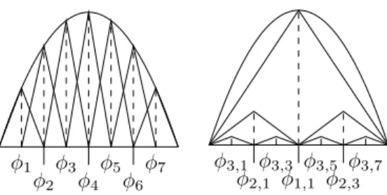
Figure 3. Comparison of piecewise linear nodal and hierarchical basis
functions on the left and right respectively. The basis functions at the endpoints are omitted as they are zero.
A. Hierarchical Surpluses
Approximations on component grids are typically com-puted and stored using a nodal basis representation, that is each elementvk in the vectorvgives the function’s value at the grid pointxk=k·2−i, that isvk =f(xk). An alternative representation is via the hierarchical basis [4] whereby each element of the vector is the difference between the function’s value’s at the corresponding grid point and the function’s values at the hierarchical neighbours. Writing v using the level notationvl,k wherel∈ {0, ..., i}and
k∈Bl=
(
{i∈N: 0< i <2l,i odd} if l >0
{0,1} if l= 0,
one has the hierarchical representation vl,k= f(xl,k)−12 f(xl−1,(k−1)/2) +f(xl−1,(k+1)/2) ! for l >0 f(xl,k) for l= 0 (3) wherexl,k :=xk·2i−l. Thesevl,k correspond to the heights of the hierarchical basis functions depicted in Figure 3. The collections {vl,k}k∈Bl for each l are referred to as
hierarchical surpluses. The hierarchical basis function in 2 or more dimensions is obtained by taking the tensor product of the one dimensional hierarchical basis functions. For full details we refer the reader to [4], [5]. Rather than perform the combination technique directly over the component grid approximations (in nodal basis) one may instead convert each component grid to hierarchical basis, combine each of the hierarchical surpluses (distributing the result) and then reconstruct the nodal basis for each component grid. This is advantageous over direct combination for two reasons: 1) it reduces the communication volume [10], 2) it allows one to avoid interpolation onto a full grid or sparse grid structure thus reducing compute cycles and memory requirements.
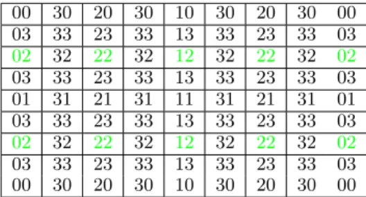
The formation of the hierarchical surpluses involves ap-plying Equation 3 across each of the dimensions of a component grid (Gi). Each element in a grid will correspond to a hierarchical surplus of index j, where j ≤i. This is
00 30 20 30 10 30 20 30 00 03 33 23 33 13 33 23 33 03 02 32 22 32 12 32 22 32 02 03 33 23 33 13 33 23 33 03 01 31 21 31 11 31 21 31 01 03 33 23 33 13 33 23 33 03 02 32 22 32 12 32 22 32 02 03 33 23 33 13 33 23 33 03 00 30 20 30 10 30 20 30 00
Figure 4. Hierarchical surplus indices corresponding to the elements of a
l= 3grid.
illustrated for i = (3,3) in Figure 4. The hierarchization process occurs in-place, with the surpluses computed from the initial grid values.
Consider the hierarchization across the x dimension in row 0. The elements with hierarchy 30 are formed by subtracting the average of the elements at distance 1 to the left and right (‘30’ is a shorthand for ‘(3,0)’). Then elements with 20 are formed by subtracting the average of the elements at distance 2 from right or left. Finally, the single element of hierarchy 10 is computed by subtracting the average of the elements in hierarchy 00 at a distance 4 to the left and right.
B. Truncated Combinations
Our SGCT algorithms support so-called ‘truncated’ com-binations [11], which avoids using the highly anisotropic grids (e.g. G(1,l)) close to the axes of the grid index
space. This avoids the problem of minimum dimension size imposed by some applications [7]. Furthermore, the highly anisotropic grids have been known to contribute least towards the accuracy of the sparse grid solution or cause convergence problems [11], enabling us to concentrate process resources on the more accurate sub-grids. Finally, it removes the limitation that the approximated full grid need not be isotropic, i.e. have an index of (l, l).
In this context we use a different notion of level to that described above in describing how much smaller the sub-grids are relative to some full gridGi0. In particular, a level l≤min{i0
x, i0y}combination in this context consists of sub-grids from the index set:
I= (ix, iy) : (i0x−l, i0y−l)< i i0x+i0y−l≤ix+iy≤i0x+i0y+ 1−l . (4) It can be noted from the above that the truncated com-bination formula is a generalization of the standard SGCT formulation, which hasi0= (l, l).
III. PARALLELSGCT ALGORITHMS
In this section, we present first the direct and then the hierarchical surplus based algorithms. Finally, we discuss their current limitations and how they may be extended.
These algorithms have a succinct description when ex-pressed via d-dimensional vector arithmetic, and we use the following notations (explained for the case d = 2). Given M, N ∈ Nd, and a ∈ N, then M ≤ N means
(Mx ≤ Nx) ∧(My ≤ Ny) and a ≤ N means (a ≤ Nx)∧(a≤Ny). Also M∗N = (Mx∗Nx, My∗Ny)and a∗N = (a∗Nx, a∗Ny). This applies to all other (integer) arithmetic operators, which include%and ==(which have the same meaning as in the C language). We also use the vector to scalar notations Σ(a) and Π(a) for the sum and product of elements of a, i.e., Σ((ax, ay)) =ax+ay and
Π((ax, ay)) =axay in the 2D case.
Crucial to their description (and to the reliable construc-tion of their implementaconstruc-tions [12]) are the mappings of global grid lengths and offsets to local lengths and offsets (which break down in turn to process offsets and index offsets within a process). If p∈ Nd is the id of a process on a process grid of size P, with 0 ≤ p < P, and given
ˆ
N ∈Ndwith0≤N < Nˆ , and lettingn=N/P, we define
the following vector functions for a block-distribution ofN overP:
l(N, p, P) = n+ (p==P−1)∗(N%P) (5)
g0(N, p, P) = p∗n (6)
p( ˆN , N, P) = min( ˆN /n, P −1) (7)
o( ˆN , N, P) = ( ˆN /n==P−1)? ˆN−n∗(P−1) : Nˆ%(8)n where l(N, p, P) is the local size of N on process p, g0(N, p, P) is the global index of the 0th local point on
p,p( ˆN , N, P) is the id of the process holding global point ˆ
N, ando( ˆN , N, P)is the local offset of global pointNˆ on that process.
The above assumes thatN ≥P. We now introduce what we will call thesparse block distributionwhich covers also the caseN < P:
ls(N, p, P) = (N >=P)?l(N, n, P) : ls(N, p/2, P/2) = (N >=P)?l(N, n, P) : (p%r== 0) (9)
g0s(N, p, P) = (N >=P)?g0(N, p, P) : g0s(N, p/2, P/2) = (N >=P)?g0(N, p, P) : r (10)
where r = Np−1. The above formulations assumes P and N−1 are powers of 2. The sparse block distribution arises when we take power of two sub-vectors from a block distribution, as for example when forming hierarchical surpluses (see Figure 4). When the sub-vectors become smaller than the process grid, we effectively form a new process grid where the processes holding no elements of the sub-vector are removed.
A. Direct SGCT
The presentation of our SGCT algorithm begins first with the scaled addition of a single sub-grid component into
Figure 5. Figure 4 from [12]. Message paths for the gather stage for the classic 2D combination method (not truncated) on a level 5 sparse grid.
The sparse grid and component grid (3,3) have2×2 process grids, all
others have2×1or1×2process grids.
the combination solution. Each sub-grid is assumed to be distributed over an independent set of processes, arranged in a d-dimensional logical grid. The combination solution is similarly distributed over a logical process grid. The parallelization of this over each component grid forms a gatherstage. This is illustrated in Figure 5. For computations performing the SGCT repeatedly, it is necessary to reverse this process by sending the respective points of the combined grid back to the component sub-grids. This is called the scatterstage, and can be visualized by reversing the arrows in Figure 5.
1) Single Sub-grid Components: Consider the scaled ad-dition of a single grid into a full grid representation of the combination uC
I ← uCI +ciui in Equation 1. For brevity, we write this as u0 ←u0+cu. LetN, N0 ∈Nd represent
the global sizes of u and u0, respectively. For the SGCT, the elements of N −1, N0 −1 will be powers of 2 and (N0−1) =r∗(N−1), where r∈Nd.
Assume u and u0 are distributed over process grids of sizeP andP0, respectively (P, P0 ∈Nd, 0< P ≤N and
0< P0≤N0).
On process p, the gather of u to the appropriate pro-cess(es) on P0 is described in Algorithm 1. The loop structure is shown ford= 2; this generalizes in the obvious way for d > 2. The number of messages sent is bounded by Π((P0+P−1)/P + 1). On line 9, note that a volume of grid points of size dn+ 1 is sent: an extra uppermost
1 Nˆ0 =rg0(N, p, P); 2 p0 =p( ˆN0, N0, P0); ˆo0 =o( ˆN , N0, P0); 3 i=0; n=l(N, p, P); 4 whileix< nxdo 5 whileiy< ny do 6 o0= ˆo0∗(i==0); // local offset @ p0 7 n0=l(N0, p0, P0)−o0; // local size @ p0
8 dn= min(n0/r, n−i); // local size here
9 send local pointsi:i+dnof utop0; 10 iy+=dny; p0y++;
11 ix+=dnx; p0x++;
Algorithm 1: Sending ofuby process pto be
gathered by the corresponding processes on P0. row and column of points is required for interpolation. It is assumed thatuhas storage for itsn points plus a ‘halo’ of neighbouring points to the positive direction, and that these have been filled by a halo exchange operation from the corresponding processes in P prior to the start of the algorithm.
The receipt on processp0 of the gridu(with combination coefficientc) and its interpolation intou0 is essentially the mirror image of this and is described in Algorithm 2. The number of messages received is bounded byΠ((P+P0−
1)/P0+ 1).
These algorithms are general for arbitraryP; as expressed here, it assumes that onP0,g0(N0, p0, P0) %r= 0, that is,
the global indices of the 0th points on p0 are a multiple of r. This is satisfied for the SGCT if the elements of P0 are powers of 2.
2) Overall SGCT Algorithm and Repeated SGCT Sup-port: Algorithm 1 is run in parallel on each Pi, and Algorithm 2 is run iteratively overi(i.e. for each sub-grid) on P0. To support the latter, arrays over i containing the process grid (Pi), grid index and combination coefficient of each grid are maintained over all processes inP0.
Our implementation can take advantage of
MPI_Irecv() semantics by allocating different buffers
(u) for each grid i, and overlapping the interpolation with the receipt of messages.
Where repeated combinations are performed, it is neces-sary to scatter back the points of the combined grids (with appropriate down-sampling) on P0 iteratively to each sub-grid onPi. It is assumed that the processes inPi have been restored by this stage if there was a failure inuidetected for the gather stage. The scatter send stage onP0is identical to Algorithm 2 except that lines 10–11 are replaced with:
sample pointsi:i+dn0−1 of u0 intou;
1 Nˆ =g0(N0, p0, P0)/r; 2 p=p( ˆN , N, P); ˆo=o( ˆN , N, P); 3 i=0; n0 =l(N0, p0, P0); 4 whileix< n0x do 5 whileiy< n0y do 6 o= ˆo∗(i==0); // local offset @ p 7 n=l(N, p, P)−o; // local size @ p
8 dn0= min(r∗n, n0−i);// local size here
9 n= min(n, dn0/r); //
corresponding size @ p
10 receiven+ 1 points frompintou;
11 interpolatec∗uinto pointsi:i+dn0−1 of u0;
12 iy+=dn0y; py++; 13 ix+=dn0x; px++;
Algorithm 2:Receipt of sub-grid uon processp0
from the gather stage from the corresponding processes on P.
send the npoints ofutop;
The receipt of the scatter occurs in parallel over each process grid Pi. The algorithm is identical to Algorithm 1 except line 9 becomes:
receivednpoints fromp0 into v; store v into pointsi:i+dn−1 ofu;
3) Partial Sparse Grid Data Structure for Efficient Inter-polation: On the receive stage of the gather operation, if we use a full grid representation of the combined grid u0, the interpolation stage (line 11 of Algorithm 2) will involve interpolating onO(2l−1)points in the full grid which are not represented by any point in any of the component grids. This is wasteful as these points are never used (in thesamplestep, above), in terms of both time and space, and furthermore this overhead is exponential in l.
This can be avoided by interpolating onto a sparse rep-resentation of u0. However, when using the truncated com-bination formula (Equation 4), the resulting data structure will be a generalization of both a regular full grid (l = 1) and a (classical) sparse grid (l = i0x = i0y). We call this representation apartial sparse grid, which represents exactly the union of points in all component grids. This section will describe how to create a distributed data structure for a partial sparse grid and the resulting interpolation and sample algorithms.
Figure 6 gives a visualization of this data structure for level l = 3 onto grid Gi0 where i0 = (4,4,4). This introduces a ‘fill-in’ factor f = i0 −l = (1,1,1) where any gaps of size 2f in from the corresponding sparse grid
(a)z= 0,4,8,12,16 (b) z= 2,6,10,14 (c)z= 1,3, . . . ,15
(c= 1) (c= 2) (c= 4)
Figure 6. Partial Sparse Grid for levell= 3SGCT onto grid (4,4,4), shown in slices across thezplane. ‘Filled in’ points (and planes) are shown in
green, with points from the sparse grid (4,4,4) in black. The compression factorcindicates the actual distance between neighbouring xy-points on the
edges.
are filled in (as far as this is possible). Note that the smaller planes must be compressed first so that there are no gaps in their boundary points.
We use concepts similar to the CSR format for sparse matrices, except we take advantage of the regularity of the partial sparse grid to avoid column indexes. Recall that this corresponds to a full grid of size N0 = 2i0 + 1. In the 2D case, global row i, 0 ≤ i < Ny0, will have global length Nx0(i) = 2i
0
x−l+l(i)+ 1, where l(i) = Z(2i+1 + 2l) and
Z(n)gives the number of rightmost zeroes before the first 1 bit inn >0. The stride between the consecutive elements in this row that must be stored is2l−l(i).
The local length in the x-dimension on process p0 of process gridP0 of the partial sparse grid is then given by
nx(i) =ls(Nx0(i), p 0 x, P
0 x)
where we are now using the scalar (d = 1) version of Equation 9. We need to use this equation as nowN0
x(i)< Px0 is possible and hence we now need to assumePx0 is a power of 2.
Process p0 computes these lengths for the n
y =
l(Ny0, p0y, Py0) rows beginning from local point 0 (global point i =g0(Ny0, p0y, Py0)) and creates the required storage vectoru0 and a row index vectorrx[0..ny−1]accordingly. It caches the corresponding row strides ins[0..ny−1].
Algorithm 3 gives the resulting code for the local interpo-lation step. It requires both alignment and scaling to take into account the grid row stride (s[i0]). These calculations in turn assume that the first local element in each row corresponds to a global (full grid) index which is a multiple ofs[i0]; this will be the case ifPx0 is a power of 2, as assumed previously. The sample operation (Algorithm 4) iterates over the elements of the component grid instead of the partial sparse grid.
To generalize this to 3D, thezandydimensions takes the place ofy andx, respectively, in the above. For thejth row inyofith plane inz, the global length of this row is given by Nx0(i, j) = 2i0x−l+l(i,j)+ 1, wherel(i, j) =Z(2j+1+ 2l(i)). 1 for(i= 0; i < n0y; i++) do 2 i0 =i+i0y; s=s[i0]; 3 j0 = (s−i0x%s)%s; j00=di0xs e; 4 for(j= 0; j <dn 0 x−j0 s e; j++)do 5 i˙=bri yc; ˙j=b j0+j∗s rx c;
6 add interpolant of c∗u[˙i..i˙+ 1,j..˙ j˙+ 1]onto u0[rx[i0] +j00+j];
Algorithm 3:Interpolation of part of a 2D component
griduof sizen+ 1, corresponding ton0 points and local offset i0of the full grid, onto the partial sparse gridu0.ris the ratio of full to component grid sizes, andn0 =r∗n.cis the component grid’s combination
coefficient. 1 for(i= 0; i < ny; i++) do 2 i0 =i∗ry+i0y; s=s[i0]; 3 j00=di0x s e; 4 for(j= 0; j < nx; j++) do 5 u[i, j] =u0[rx[i0] +j00+j∗rx/s]; // note: s|rx and rx≥1
Algorithm 4: Samplenpoints from local full grid
offseti0 from partial sparse grid u0 into part of a component gridu.ris the ratio of full to component
grid sizes.
4) Support for Fault Tolerance: As described in [7], the classical SGCT algorithm can be made fault-tolerant with alternate combination formulas requiring the inclusion of extra diagonals (2D) or planes (3D). Before the SGCT is applied, failed processes are detected and recovered, and the grids of the failed processes are allocated a combination coefficient of c = 0. Assuming that these processes were associated with gridi, the gather ofui onPi andP0 is not performed.
As mentioned in Section III-A2, the abstraction of having a simple array of grid data means that the algorithm is
effectively oblivious to the extra requirements for a fault-tolerant SGCT.
B. Hierarchical Surpluses-Based Algorithm
An alternate approach to the SGCT is to form the hi-erarchical supluses on each component grid. This can be done in-place, as observed in Section II-A and this can occur in parallel over each component grid’s process grid (P). Then, for each surplus h ∈ Nd, where h ≤ i0, the
(direct) SGCT is performed on each. Only the processes holding part of surplus h need participate, that is those holding the component grid Gi, where i ≥ h. Finally the original component grids can be recovered from the combined surpluses, thus performing an overall SGCT.
Only surpluses common to more than one grid need be combined. For 2D, this is for hierarchyhsatisfying:
H2(x, y) :hx+hy <=i0x+i 0 y−l
This is illustrated in Figure 7. For 3D, the condition be-comes:
Σ(h)<= Σ(i0)−2l+ 1∧H2(x, y)∧H2(x, z)∧H2(y, z) As the number of hierarchies is O(Π(i0)), applying the SGCT on them individually is likely to suffer from high startup overheads.
In this section, we describe a parallel algorithm for forming the surpluses (and recovering the original grid from its surpluses). This is followed by a description of how to coalesce these hierarchies, in order to try to reduce startup overheads, and how to schedule them where possible in parallel. We then describe how to overcome an issue with this approach, that is how to handle the case where a hierarchy becomes too small for a process grid P > 1, noting hierarchy his of size2h−1 for h >0. Our solution
is called process sub-griding. Finally, we present how the direct SGCT algorithm was extended to operate on coalesced surpluses.
1) Formation of Hierarchical Surpluses: Let P ∈ Nd denote the process grid over which component grid Gi is distributed and N ∈ Nd be the global size of this grid
(N = 2i+ 1). Algorithm 5 gives the corresponding parallel algorithm for the 3D case (which can easily be generalized for higher dimensions). The notationN\dx∈Nd denotes a
vector with the same elements asNin all dimensions except d, where it has a value ofx∈N.
First, we calculate the global left and rightmost global indices of points on processp(line 1). We iterate over each dimension (line 2) and then over each stride length of the hierarchies of that dimension (line 3). Note that the index for the hierarchy is given byh=id−s. Then, we calculate the global indices of the leftmost and rightmost source points for this surplus (lines 4–5). With this, we calculate the surpluses for local points which do not need points from neighbouring processes (lines 6–7). “Plane j of u” should be read as
1 Nl=g0(N, p, P), Nr=Nl+l(N, p, P)−1; 2 ford=x, y, zdo 3 fors= 0 :id−1 do 4 jl=Ndl + min{x≥0|(Ndl+x)%2s+1= 0} 5 jr=Ndr−min{x≥0|(Ndr−x)%2s+1= 0} 6 forj=jl+ 2s:jr−2s: 2s do 7 hierarchize planej ofu 8 kl =jl−2s;kr=jr+ 2s 9 if 0≤kl< Ndl ≤jl≤Ndr then 10 send planejl ofutop(Nl\dkl, N, P) 11 if Ndl ≤jr≤Ndr< kr< Nd then 12 send planejr of utop(Nr\dkr, N, P) 13 if Ndl ≤kl≤Ndr then
14 receive plane from p(Nl\d(kl−2s), N, P) 15 hierarchize planekl of u, if kl6=kr 16 if Ndl ≤kr≤Ndrthen
17 receive plane fromp(Nr\d(kr+ 2s), N, P)
18 hierarchize planekrof u
Algorithm 5: Hierarchization of griduof global size
N = 2i+ 1by processpin process gridP.
“plane of global index j in dimension d of u”. Note that the local index onpis given simply byj−Nl
d. If powns the leftmost source pointjl and another process on the left
holds the next destination pointkl, we send planejl to that
process, and similarly forjr (lines 8–10). Ifpownskl then
we receive the plane kl −2s from the owning process on the left and planekl can now be hierarchized, and similarly
forkr (lines 13–18).
To restore the original grid from the surpluses, we simply reverse the order of the stride loop (line 4), and add instead of subtract the averages of the source points (line 7, 15 and 18).
2) Scheduling and Coalescing of Surpluses: A set of hierarchies may be coalesced without introducing redundant communications if they are present on a common set of component grids. This is illustrated for a 2D example in Figure 7, which shows the index spaces for each surplus can be coalesced under this principle. The component grids are indicated in yellow; indices on the upper boundaries (dotted) are common to only one grid and need not be combined.
The surpluses may be combined in the following order. Surpluses (i0
x−l+ 1, i0y−1), . . . ,(i0x−1, i0y−l+ 1) are combined (separately) first, then those of the next diagonal in the triangular area, until finally surplus(i0x−l+1, i0y−l+1). It should be noted that each surplus in this triangular area operates on different sets of component grids, and so may not be coalesced with another (without causing redundant communications). Then we combine the surpluses coalesced
Figure 7. Coalesced hierarchical index spaces for a 2D truncated SGCT
with l = 5 and i0 = (9,9). Indices of 0 are are not shown. The
corresponding indices of the component grids are filled with yellow. Indices to surpluses common to only one grid are in dashed boxes. Note that the size of the corresponding surplus halves as an index is decreased by 1.
in one dimension,(0 :i0x−l, i0
y−1), . . . ,(0 :i0x−l, i0y−l+1) and(i0x−1,0 :i0y−l), . . . ,(i0x−l+ 1,0 :i0y−l), and finally those coalesced in both(0 :i0x−l,0 :i0y−l). This coalescing is possible as they reside on common sets of the component grids.
While the avoidance of communicating the surpluses com-mon to only one grid ((i0x−l+1, i0y), . . . ,(i0x, i0y−l+1)) is an advantage of this approach, it has a drawback in that there is limited parallelism over the whole system. This can be min-imized if surpluses i along each diagonal in the triangular area at a distanceδ(i) =i0x+iy0 −l+ 2−(ix+iy)apart are scheduled in parallel, as they share no common component grids. For example, in Figure 7, along the diagonal beginning with (8,5), δ(i) = 2, and surpluses marked ‘1’ may run in parallel, as may those marked ‘2’. Similarly, for the surpluses coalesced in one dimension, if these are scheduled from biggest to smallest, i.e.(0 :i0x−l, i0y−1),(i0x−1,0 :
i0y−l),(0 :i0x−l, i0y−2),(i0x−2,0 :i0y−l), . . ., then the firstbl/2c −1 of these pairs operate on disjoint component grids and hence will run in parallel. This is illustrated in in Figure 7 with the coalesced surpluses marked ‘3’. It should be noted that (coalesced) surpluses need to have the same size if they are to be effectively scheduled together.
For 3D, the generalization involves the combination of (l−1)(l−2)(l−3)/3,3(l−1)(l−2)/2,3l and 1 groups coalesced in 0, 1, 2, and 3 (respectively) dimensions. The scheduling distanceδ(i)increases by 1. This, combined with
the fact that the average diagonal is shorter, means that the average scope of parallelization of coalesced surpluses markedly diminishes from the 2D case.
3) Extension of Direct Algorithm to Support Surpluses: We now consider how the SGCT can be applied to the hierarchical surplus h ∈Nd, for which the boolean vector
¯
c ∈ {0,1}d indicates that it is notcoalesced with all lower indices in each dimension.
Let the current process hold part of grid Gi of sizeN=
2i+ 1, with an associated process grid P, and this process has id pon this grid. If h≤i does not hold, surplus his not inGiand the process participates no further. Otherwise, the process proceeds with the corresponding grid index for the SGCT given byh0=h−¯c.
The (local portion of the) surplus must first be extracted. The relevant parameters of are the stride s, global index offsetO, local index offset oand the local lengthn:
s = 2i−h−c¯
O = ¯c∗s/2
o = min{v≥0|(g0(N, p, P)−O+v)%s= 0}
n = (l(N, p, P)−o+s−1)/s+ (p==P−1)∗c¯ The last term for n represents a padding required for an uncoalesced surplus, since these have a global size which is exactly a power of 2. We can also compute nby
n=l(N0, p, P), where N0= 2h0+ 1
The elements of the extracted surplus may be now sup-plied to the direct SGCT algorithm, which has h0 (N0) set to both the component and combined grid index (size) for the current combination.
The SGCT algorithm is also set into hierarchical mode. In this mode, computations over all the original component grids must skip any grid not containing the hierarchy h0. Here, the grid ratior= 1and we senddninstead ofdn+ 1 points (line 9 of Algorithm 1), as interpolation and hence boundary points are not required. Finally, the combination process grid P0 in this case may only involve processes participating in the current combination, which will be a subset of the processes operating on all component grids.
4) Process Sub-griding: Even with the coalescing of hi-erarchical surpluses, a component gridGi that is distributed of a process grid P can have a hierarchyhthat is, in some dimensions, smaller than the process grid. In this case, the regular block distribution breaks down and the direct SGCT algorithm cannot be applied. Figure 8 illustrates this case whereP = (8,8). It can be observed however that here we still have a sparse block distribution(see Equations 9–10), and that, if we take a sub-grid of P beginning at process offset (0,2) and stride (2,4), the hierarchy will retain a block distribution over that sub-grid. An exception occurs for the rightmost elements of the hierarchy, where the process stride is 1.
00 30 20 30 10 30 20 30 00 03 33 23 33 13 33 23 33 03 02 32 22 32 12 32 22 32 02 03 33 23 33 13 33 23 33 03 01 31 21 31 11 31 21 31 01 03 33 23 33 13 33 23 33 03 02 32 22 32 12 32 22 32 02 03 33 23 33 13 33 23 33 03 00 30 20 30 10 30 20 30 00
Figure 8. Hierarchical surplus indices corresponding to the elements of a
l= 3grid, highlighting coalesced hierarchy(0 : 2,2)on an8×8process
grid.
1 q=r; // r is the 1D rank of this
process in P 2 ford=x, y, z do 3 p0d= (q−Od)%Pd; δ= (p0d==Pd−1)∗Zd; 4 if(p0d+δ)%sd== 0 /*is part of sub-grid*/then 5 p0d= (p0d+δ)/sd; q=q/Pd;
Algorithm 6:Determination of sub-grid process ids
Our solution to this problem is to form such a sub-grid and allows only the processes that are part of it to participate in the SGCT. The following calculations determine the process offset, stride and ‘zero delta’ and size of the process sub-grid:
s = (P <= 2h)?1 : (h== 0)?P :P/h O = ¯c∗s/2
Z = (1−c¯)∧(s >1)
P0 = min(P,2h+ (h >0)∗Z)
Algorithm 6 can be used to determine if a process of P is in the sub-grid and, if so, its id within that sub-grid. C. Limitations and Extensions
As noted at the end of Section III-A1, the elements on sparse grid process grid (P0) currently need to be powers of 2 for the direct algorithm. This can be relaxed if the halo points of uhave also been filled in the negative direction, and pointsi−1 :i+dnare sent at line 7 of Algorithm 1 andn+ 2points are received on line 10 of Algorithm 2 and included in the interpolation (line 11).
The hierarchical surplus algorithm however requires all component process grids sizes (P) to be powers of 2. This is because the surpluses have a power of two stride (see Figure 4); thus the elements of the surpluses will only retain a block distribution (Equations (5–8)) in this case. This could be overcome at the expense of redistribution.
Our current implementation can accommodate 2D or 3D combinations. The main engineering issues in extending it to a higher dimension dare (i) for a given level l, the number of sub-grids increases rapidly with d (so load balance in the underlying SGCT application will become an increasing concern), (ii) enumerating the grid indices for these sub-grids across the hyperplanes in grid index space becomes increasingly complex and (iii) the sparse grid data structure becomes increasingly complex. For the hierarchical surplus algorithm, the enumeration of the coalesced surpluses sub-spaces (Section III-B2) also becomes increasingly complex. As mentioned in [7], the implementation of our algorithms supports a 2D or 3D SGCT on 4D or higher-dimensional grids. A lower dimension (say of size b) than those used for the SGCT is supported by extending the implementation to handle blocks of b elements. Higher dimensions can be dealt with by applying the SGCT iteratively. The dimensions chosen for the SGCT must be contiguous, and a local transposition can be applied in order to ensure this.
Our direct SGCT algorithm supports parallelization over arbitrary process grids (Pi) in the SGCT dimensions of a data grid. As also explained in [7], parallelization in a non-SGCT dimension can be simply performed by applying the whole SGCT in parallel over this dimension.
IV. ANALYSIS
We now will give an analysis of our SGCT algorithms un-der typical operating conditions imposed it with conjunction with an application [9], [7].
In order to perform a SGCT over the desired set of sub-grids {ui}, where ui is distributed over the process grid Pi, we form the combined process grid P0 over a subset of these processes. That is, Π(P0) = 2k for the largest k such that 2k ≤Σ
iΠ(Pi). The aspect ratio ofP0 will be set to match the grid index of the combined (full) grid. In this case P0 ≥Pi. For simplicity (and because it is a case of strong practical interest [9], [7]), we assume each Pi is a power of 2 also.
In terms of load balancing, we allocate the same number (p ∈ N) of processes on each of the Pi on each diagonal in the grid index space (see Figure 2); in the 3D case, the diagonal becomes a plane. The next lower diagonal receivesdp/2eprocesses. This strategy balances the amount of data points and hence work across each processes, which approximates to a first order the load for that process.
We denoteg=g(d, l)to be the number of sub-grids given dimensionalitydand levell. We haveg(d, l) =O(ld−1)and
more specifically:
g(2, l) = 2l−1 (11)
g(3, l) = 3l2−2l+ 1 (12) Let m denote the number of data points in a sub-grid in a given process. By the above assumptions m should be constant across all processes. Let αand β denote the cost
of starting up a message and the transmission cost per unit data.
A. Direct SGCT Algorithm
For this algorithm, in the worst case, each process in P0 will receive2mwords of data. Each process in eachPisends and receivesΠ(P0/Pi)≤g messages, and each process in P0 receives and then sends g messages. Since the whole operation should be completely parallelized, the total cost of the direct gather-scatter is given by:
td≤2gα+ 3mβ (13)
This indicates that the algorithm should be efficient in bandwidth-constrained (largem) circumstances, which will be the case for most large-scale simulations. Otherwise, when g is large, it may be less efficient compared to an algorithm based on multistage reductions with a constant fan-in [10], with a cost of2 log2(g)(α+mβ).
B. Interpolation Overheads
Consider a levellSGCT on ad-dimensional isotropic grid of grid indexi0∈N,i0≥l. The full grid will haveO(2i
0d ) points. The partial sparse grid will have a fill in factor of f(d, l) = 2(i0−l)d and hence will have
f(d, l)2lO(ld−1) = 2i0d−(d−1)lO(ld−1)
data points, noting a classical sparse grid (i0 = l) has 2lO(ld−1) points. Each component grid will have 2i0d−(d−1)(l−1) points.
Assume the upper level grids are distributed across p processors, and partial sparse grid is distributed over the total number of processors,g(d, l)p=O(ld−1)p, using Equations
11–12.
Then the ratio of partial sparse grid to component grid points per process is given by:
2i0d−(d−1)lO(ld−1)/(O(ld−1)p) 2i0d−(d−1)(l−1)
/p = O(1)
This indicates that the interpolation stage should scale with p, l, andd. However, the number of interpolation calculations per received point is O(ld−1) and hence, for sufficiently
large l and d, interpolation time will dominate communi-cation time.
By contrast, if a full grid is used for interpolation, the ratio of full grid to component grid points per process is
2i0d/(O(ld−1)p) 2i0d−(d−1)(l−1)
/p = 2
(d−1)(l−1)/O(ld−1)
which is essentially exponential inl.
C. Hierarchical Surplus-based Algorithm
This approach avoids communication of surpluses shared by only one grid, which reduces the total communication volume by a fraction 1
2d. This is however offset by both
the limited parallelization and load imbalance imposed. Furthermore, even with coalescing, the overhead of com-munication startups will be considerably increased over the direct method. This will however be partially offset by the average effective value of g being ≈30% on average less. For example, the direct algorithm should should perform fairly optimally, given Equation 13, on the largest surpluses, which have a minimal g= 3.
Roughly the load imbalance factor will be ≈2d−1, due
to the fact that process grids on the inner diagonal (see the highlighted areas of Figure 7) have half the number of processes, but the sizes of the surpluses is the same across all grids. The average degree of parallelization will be≈2/3 for the scenario of Figure 7. Consider the largest surpluses, labelled ‘1’ and ‘2’. Those labelled ‘2’ cannot run in parallel with those marked ‘1’. Those marked ‘3’ can run in parallel, but then only≈2/3of the processes can be utilized. As we move closer to the origin, the overall utilization increases, till it is1when the indices are less thani0−l+ 1(= (5,5) in the figure). However, these areas represent only a small fraction of the overall data.
A more precise analysis needs to be done empirically. Included in the code release for this work is a Python script calculating the overall degree of parallelization for the combination of all surpluses. This generated the data for the following table, for the 2D case i0 = (9,9) with coalesced supluses:
scheduling\l 3 4 5 6 7 8 9
yes 0.80 0.82 0.74 0.75 0.72 0.72 0.70 no 0.80 0.69 0.62 0.58 0.54 0.52 0.50 This indicates that scheduling should make a worthwhile difference, achieving a 70–80% degree of parallelization. An experiment where the grid size grows withl, i.e. i0 = (9 + l,9 +l), gave essentially identical results.
Taking all these factors together, it is unclear if this approach, even with scheduling, has any overall inherent advantage in speed even ford= 2.
V. EXPERIMENTALRESULTS
In this section, we give performance results for our algorithms, under the operating conditions mentioned in Section IV.
All experiments were conducted on the Raijin cluster located at the Australian National University. It has 3,592 compute nodes, consisting of dual 8-core Intel Xeon (Sandy Bridge 2.6 GHz) processors (i.e. 16 cores) with on average 44 GB memory per node, and with an Infiniband FDR interconnect (56Gbs). Version 1.4.3 of Open MPI was used
and our codes were compiled withgcc4.6.4 with the-O3
option.
A. Direct SGCT Performance
In order to demonstrate the effect of our parallel SGCT algorithm on an application, we use an advection solver capable of solving 2D and 3D problems. As the amount of work per timestep for the advection problem is relatively small compared to most real applications, any inefficiencies in the SGCT will be easily seen.
Figure 9 shows strong scaling results. The plots BSend indicate an MPI_BSend based implementation was used:
this imposes a fixed order of message receipt. The plots ISend indicate that anMPI_ISend/IRecvimplementation
was used, which does not have this limitation and allows the overlap of communication with the interpolation of the gather stage. For the 3D problem, results for small core counts are missing for the former, as the MPI implemen-tation was not able to handle the very large BSend buffers that were required.
The results indicate that the application scales even with the SGCT applied relatively frequently, with the ISend implementation lending ≈ 20% extra performance to the overall execution time.
Figure 10 indicates the weak scaling performance of the direct 2D SGCT in isolation using the partial sparse grid data structure (the default). We chose 214 points per
process as this represents a reasonable amount of data, and is sufficiently large so that the bandwidth components of the SGCT (see Equation 13) becomes significant. It indicates that once communication is predominantly inter-node, the execution time remains relatively flat, indicating good scaling performance to the limit of our tests at around 3000 cores.
It can be noted that execution time increases slowly with increasing l when the sparse grid data structure is used (Figure 10(b)). At l = 3 and l = 11, the total core counts are an exact power of two; this is the best case for the algorithm, as all cores can hold part of the partial sparse grid. We have some performance loss at l = 5, l = 7 and
l = 9 where only 80%, 76% and 88% of the cores hold part of the sparse grid. There is approximately a factor of 2 between the performance atl= 3andl= 11cases. Much of this difference is due to the interpolation time (’in’), whose proportion of overall execution time increases withl. This is largely due to load imbalance effects: the sparser the (partial) sparse grid becomes, the less evenly the points divide over a regular process grid. As can be seen from Figure 1, the processes at the corners may have significantly more points than their neighbours towards the interior.
Figure 10(a) shows the results if the much simpler full grid data structure is used for interpolation. This introduces a factor of ≈2l−1 redundant data points. As expected, we
get an exponential increase in execution time with respect to
l, with interpolation time quickly accounting for almost all execution time. It indicates that the sparse grid data structure is essential for good scaling with l.
While interpolation appears to account for much of the total time, it should be noted that message receipt is over-lapped with it, hence message receipt time is attributed to interpolation time. Results corresponding to Figure 10(a) for the BSend implementation indicate that interpolation never consumes >50% of execution time. They also show poorer scaling with core count than the ISend results. Other experiments indicate the partial sparse grid interpolation function achieves near-ideal thread-level parallelism.
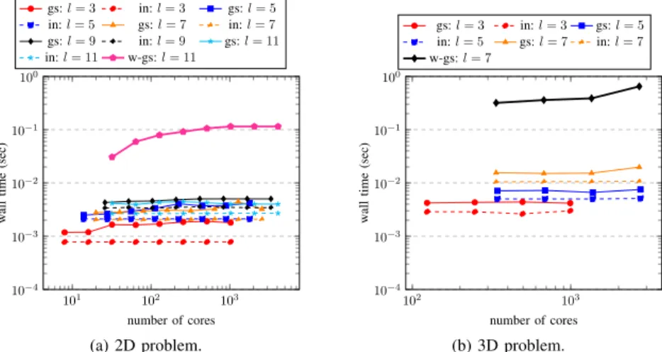
Figure 11 gives a comparison of the 2D and 3D algorithms using the sparse grid data structure. In terms of the number of component grids, l = 3,5,7 in 3D is equivalent to the cases l = 5,17,31 in 2D. We can see that 2D and 3D performance is very similar for l= 3(3D) andl= 5 (2D), and 3D scales similarly well with increasing core count. We also see a gradual decrease in performance as the number of component grids increases becomes large, due to the increased effects of startup latency.
All data shown so far are for ‘warmed’ timings where an SGCT was performed before the timing was taken. Figure 11 shows the time for the direct SGCT without this warmup; we see a degradation in performance by a factor of approximately 20. This is caused by OpenMPI setting up new (inter-grid) connections between processes in order to perform the SGCT. While not part of the SGCT itself, this overhead needs to be taken into account by any application using the SGCT. The results of our previous work [13] do not take this effect into account.
B. Hierarchical SGCT Performance
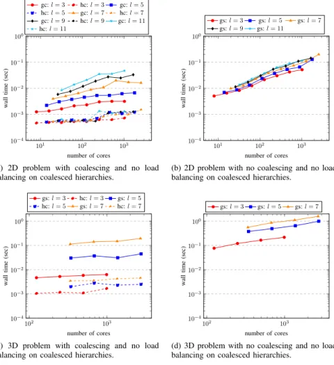
Figure 12 indicates the performance of the hierarchical surplus based algorithms. A comparison of sub-figures (a) to (b) and (c) to (d) indicates the clear benefit of coalescing the surpluses. Comparing sub-figures(a) and (c) to Figure 11, we see that this version is slightly slower for smallerl and core counts. We also see that it scales less well with l, due to the fact there areO(l2)sub-operations and the number of
cores (especially as g(l)increases). Somewhat surprisingly, scheduling of the surpluses gave no clear overall benefit.
The forming and restoring from the hierarchical surpluses formed a small factor (≈ 1/10) of this. As expected, the results vary little with l for 2D, but show some increase withl for 3D.
It should also be noted that there are no other SGCT codes available that can be used to perform the above experiments for comparison.
C. Load Balance and Communication Profiles
Figure 13 gives IPM profiles [14] for the 2D advection application with a l = 11 SGCT. We can clearly see the structure of the advection sub-problems. MPI_Send and
44 88 176 352 704 1408 1 10 number of cores ov erall ex ecution time (sec)
Isend: 1×comb Bsend: 1×comb Isend: 4×comb Bsend: 4×comb Isend: 16×comb Bsend: 16×comb Isend: 64×comb Bsend: 64×comb
(a) 2D problem with levell= 4and213×213
grid points. 31 62 124 248 496 992 1984 1 10 number of cores ov erall ex ecution time (sec)
Isend: 1×comb Bsend: 1×comb Isend: 4×comb Bsend: 4×comb Isend: 16×comb Bsend: 16×comb Isend: 64×comb Bsend: 64×comb
(b) 3D problem with levell= 3and29×29×28
grid points.
Figure 9. Overall execution time of the advection application with the direct SGCT running over 1024 timesteps (MPI warm-up time excluded). Results shown are an average of two experiments.
101 102 103 10−4 10−3 10−2 10−1 100 number of cores w all time (sec) gs:l= 3 in:l= 3 gs:l= 5 in:l= 5 gs:l= 7 in:l= 7 gs:l= 9 in:l= 9 gs:l= 11 in:l= 11
(a) interpolation on a full grid.
101 102 103 10−4 10−3 10−2 10−1 100 number of cores w all time (sec) gs:l= 3 in:l= 3 gs:l= 5 in:l= 5 gs:l= 7 in:l= 7 gs:l= 9 in:l= 9 gs:l= 11 in:l= 11
(b) interpolation on a sparse grid.
Figure 10. Execution time of the average of 10 repetitions of the 2D direct SGCT in isolation (MPI warm-up time excluded). The workload of each core
is214grid points. ‘l’, ‘gs’, and ‘in’ denote the level of the SGCT, combination time, and the time on the interpolation step only, respectively. ISend-based
implementations are used. Results shown are an average of two experiments.
MPI_Recv are used only in the advection phase, being used for halo exchanges. The fluctuations in MPI_Waitany in part (a) indicates (inversely) load imbalance across the process grid caused by differences in computational speed across the different sets of advection problems. It is also the dominant communication time for the SGCT operation (part(b)). D. Effect of Process Grid Aspect Ratio and Process Layout on Performance
The aspect ratios of each component grid and its pro-cess grid determines the shape of the decomposed domain. Changing the decomposed domain shape and changing how processes are aid out across nodes changes the commu-nication pattern for both the computation of application on the grid and the SGCT. Each application has its own communication requirements, and so process grid aspect
ratio and layout may affect them differently. We analyze the effect for the 2D advection application with different process layouts.
The default SGCT process grid layout is made to match the shape of the component gridGi. Allocating 64 processes to the largest component grids, the default process layout for 2DGiwithi= (3,0),(2,1),(1,2),(0,3),(2,0),(1,1), and
(0,2) are 16×4, 8×8, 8×8, 4×16,8×4,8×4, and 4×8, respectively. That of the 2D full grid is16×16.
How process are mapped to nodes also affects commu-nication. The process-to-node mapping of all the previous benchmarks were done by mapping the processes to cores in nodes linearly (default), as shown in Figure 14a for a 2D process grid. This will minimize inter-node communication horizontally at the expense of inter-node communication in the vertical dimension. A block-wise mapping, such is as
101 102 103 10−4 10−3 10−2 10−1 100 number of cores w all time (sec) gs:l= 3 in:l= 3 gs:l= 5 in:l= 5 gs:l= 7 in:l= 7 gs:l= 9 in:l= 9 gs:l= 11 in:l= 11 w-gs:l= 11 (a) 2D problem. 102 103 10−4 10−3 10−2 10−1 100 number of cores w all time (sec) gs:l= 3 in:l= 3 gs:l= 5 in:l= 5 gs:l= 7 in:l= 7 w-gs:l= 7 (b) 3D problem.
Figure 11. Execution time of the average of 10 repetitions of the direct SGCT in isolation. The workload of each core is214grid points. ‘l’ represents
the level of the SGCT. ‘gs’ and ‘in’ denote the combination time and the time on the interpolation step only, respectively, when MPI warm-up time is excluded. ‘w-gs’ denote the combination time when MPI warm-up time is included. ISend-based implementations are used. Results shown are an average of two experiments.
shown in Figure 14b, will balance inter-node communication ni both dimensions.
The effect of process aspect ratio and layout for a 2D advection application is presented in Tables I and II in isolation. It is observed from Table I that8×8,8×4process grid with block map shows a small advantage in advection computation time. Applying the same configuration also improves the combination time slightly as shown in Table II.
VI. RELATEDWORK
Early work in the parallelization of the SGCT for Laplace’s equation and the 3D Navier-Stokes system was reported in [2] and [15], respectively. However, the algorithm assumed each node had multiple sub-grids and concentrated on load balancing aspects, whereas our algorithm is designed for the many processes per sub-grid case.
More recently, work on a parallel SGCT algorithm has also involved allocating multiple grids per process group of size limited to the number of cores in a socket, with OpenMP parallelism applied within each process group [8]. The algorithm was targeted towards higher dimensional problems and the concern was in load balancing within sub-groups of O(1000)grids.
Work on load-balancing of component grid instances for the SGCT and a parallel SGCT algorithm using both the direct and hierarchical surplus implementations has been reported in [16] and [10], respectively. The latter paper also gives an analysis of their algorithms’ communication overheads. However, it is assumed that there is only one process per component sub-grid (i.e. Pi = 1), severely limiting its applicability to large-scale simulations. Their algorithm also does not support the truncated combination formula. While in both cases, the (direct) algorithm is based on a gather-scatter approach at the top level, our
algorithm has only two stages, whereas theirs hasO(log2l)
stages. Furthermore, their version of the direct algorithm involves a significant amount of redundant communications, resulting in their conclusion that the hierarchical surplus approach is 10× (3.5×) faster for a high SGCT level (l) for 2D (3D) combinations. For our algorithms, we reach the opposite conclusion. The paper mentions the idea of “merging” (coalescing?) hierarchical surpluses only in the context of future work.
Efficient data structures for sparse grids usually rely on tree or hash methods [17], [18]. More recently, a more com-pact representation involving multi-level indexing of a flat array, ranged in the order of the hierarchical surpluses [19]. It also offers faster indexing. Our sparse grid data structure based on sparse matrix ideas shares these advantages and moreover has potentially better data locality, as the flat array is based on the spatial layout of the original component grid. Furthermore our implementation is more general than any, as it is fully distributed and covers partial sparse grids as well.
[9] used our 2D direct SGCT implementation to build a fault-tolerant 2D advection solver. As its emphasis was on fault-tolerance it gave no details of the SGCT algorithm nor did it examine its performance in isolation. Similarly for [12], which studied the computational complexity of the par-allel SGCT and described software engineering techniques to reduce the complexity and ensure the reliability of the 2D direct SGCT implementation. Indeed, these techniques proved even more crucial to the more complex 3D and hierarchical surplus based implementation of the algorithms presented here. However, these papers give no details about the parallel SGCT algorithm itself.
This paper is an extended version of our preliminary work [13]. The algorithms have been perfected, with details for 3D
101 102 103 10−4 10−3 10−2 10−1 100 number of cores w all time (sec) gc:l= 3 hc:l= 3 gc:l= 5 hc:l= 5 gc:l= 7 hc:l= 7 gc:l= 9 hc:l= 9 gc:l= 11 hc:l= 11
(a) 2D problem with coalescing and no load balancing on coalesced hierarchies.
101 102 103 10−4 10−3 10−2 10−1 100 number of cores w all time (sec) gs:l= 3 gs:l= 5 gs:l= 7 gs:l= 9 gs:l= 11
(b) 2D problem with no coalescing and no load balancing on coalesced hierarchies.
102 103 10−4 10−3 10−2 10−1 100 number of cores w all time (sec) gs:l= 3 hc:l= 3 gs:l= 5 hc:l= 5 gs:l= 7 hc:l= 7
(c) 3D problem with coalescing and no load balancing on coalesced hierarchies.
102 103 10−4 10−3 10−2 10−1 100 number of cores w all time (sec) gs:l= 3 gs:l= 5 gs:l= 7
(d) 3D problem with no coalescing and no load balancing on coalesced hierarchies.
Figure 12. Execution time of the average of 10 repetitions of the hierarchical SGCT in isolation (MPI warm-up time excluded). The workload of
each core is214 grid points. ‘l’, ‘gs’, and ‘hc’ denote the level of the SGCT, combination time, and the time to form and restore from the hierarchical
surpluses, respectively. As the scheduling of hierarchical surpluses does not offer significant improvement, those are not included in the graph. ISend-based implementations are used. Results shown are an average of two experiments.
(a) computing whole application: MPI task (b) performing combination: MPI task
Figure 13. Analysis of IPM generated load balance of 2D direct SGCT solving advection on level 11 with a single combination (MPI warm-up time
excluded). Core count on each upper layer grid is16. Workload per core is214points and number of timesteps is214. The total execution time is 4.06
96 64 32 0 97 65 33 1 98 66 34 2 99 67 35 3 100 68 36 4 101 69 37 5 102 70 38 6 103 71 39 7 104 72 40 8 105 73 41 9 106 74 42 10 107 75 43 11 108 76 44 12 109 77 45 13 110 78 46 14 111 79 47 15 112 80 48 16 113 81 49 17 114 82 50 18 115 83 51 19 116 84 52 20 117 85 53 21 118 86 54 22 119 87 55 23 120 88 56 24 121 89 57 25 122 90 58 26 123 91 59 27 124 92 60 28 125 93 61 29 126 94 62 30 127 95 63 31 (a) linear (default) mapping
96 64 32 0 97 65 33 1 98 66 34 2 99 67 35 3 100 68 36 4 101 69 37 5 102 70 38 6 103 71 39 7 104 72 40 8 105 73 41 9 106 74 42 10 107 75 43 11 108 76 44 12 109 77 45 13 110 78 46 14 111 79 47 15 112 80 48 16 113 81 49 17 114 82 50 18 115 83 51 19 116 84 52 20 117 85 53 21 118 86 54 22 119 87 55 23 120 88 56 24 121 89 57 25 122 90 58 26 123 91 59 27 124 92 60 28 125 93 61 29 126 94 62 30 127 95 63 31 (b) block mapping
Figure 14. 2D linear and block mapping of32×4process grid onto cores of Raijin nodes. Processes with the same color are mapped onto the cores of
the same node. Different color represents mapping onto different nodes. Table I
AVERAGE AND MAXIMUM TIME SPENT ON352 CPUCORES FOR COMPUTING ADVECTION ON COMPONENT GRIDS(MPIWARM-UP TIME EXCLUDED). A 2DDIRECTSGCTWITH LEVEL4IS USED IN THE ADVECTION APPLICATION.
adv
ection SGCT default 8×8,8×4 block map 8×8,8×4 and block map
average 4.34 4.35 4.32 4.28
maximum 4.49 4.55 4.44 4.34
Table II
AVERAGE AND MAXIMUM TIME SPENT ON352 CPUCORES FOR PERFORMING COMBINATION OF THE COMPUTED COMPONENT GRIDS(MPIWARM-UP TIME EXCLUDED). A 2DDIRECTSGCTWITH LEVEL4IS USED IN ADVECTION APPLICATION.
combination
SGCT default 8×8,8×4 block map and block map8×8,8×4
average 2.04E-02 2.03E-02 2.02E-02 2.02E-02
maximum 2.20E-02 2.23E-02 2.18E-02 2.17E-02
added, and we have introduced the sparse block distribution, the partial sparse grid data structure and the process sub-griding technique. The analysis is more comprehensive and more precise. The experimental results are all significantly improved and extended results have been included.
VII. CONCLUSIONS
In this paper, we have presented two general SGCT com-bination algorithms both supporting parallelism within and across process grids and the more general SGCT ‘truncated combination’ formula. They can also support fault-tolerant SGCT combination formulae. The algorithms are inherently complex but can be formulated (and implemented) tractably when expressed in terms ofd-dimensional vector arithmetic and the associated mappings for a block distribution. The direct algorithm is highly efficient in bandwidth-limited scenarios and is general in terms of the process grid con-figurations of the component grids. It is particularly suited to SGCT where the number of component grids is small to moderate, i.e. d≤5. It does however need a partial sparse grid data structure, a generalization of the sparse grid, to be
scalable with the SGCT levelland the dimensionalityd. Our distributed implementation of this data structure, based on sparse matrix concepts, is comparably efficient to existing non-distributed implementations, in terms of both space and access time, and scales in the same sense as the SGCT.
The hierarchical surplus based algorithm uses the direct algorithm for combining the individual and coalesced hier-archical surpluses. It thus inherits some of the performance characteristics of the direct algorithm. It offers a bandwidth reduction by a factor of 1−2−d; however, this seems to be offset by an incomplete parallelization factor ≥ 2/3 for 2D (and even this requires careful scheduling of the computation), a factor of ≈ 2d−1 load imbalance (arising from the uneven number of processes across the component grids) and overall increased startup times. The latter is reduced by our technique of coalescing the surpluses for combination. It appears to have an advantage in memory consumption, with the extra memory for the SGCT being reduced to the size of the largest common surpluses, which is a factor of2−d of the largest component grids. However, the direct algorithm can match this by partitioning the SGCT
![Figure 5. Figure 4 from [12]. Message paths for the gather stage for the classic 2D combination method (not truncated) on a level 5 sparse grid.](https://thumb-us.123doks.com/thumbv2/123dok_us/9322872.2810830/4.918.478.851.102.501/figure-figure-message-gather-classic-combination-method-truncated.webp)