On obtaining effective elasticity tensors
with entries zeroing method
Bartosz Gierlach, Tomasz Danek
AGH University of Science and Technology, Faculty of Geology, Geophysics and Environmental Protection, Department of Geoinformatics and Applied Computer Sciences; al. A. Mickiewicza 30, 30-059 Krakow, Poland; e-mail: [email protected], [email protected]
© 2018 Authors. This is an open access publication, which can be used, distributed and reproduced in any medium according to the Creative Commons CC-BY 4.0 License requiring that the original work has been properly cited.
Received: 21 August 2017; accepted: 25 April 2018
Abstract: The purpose of this paper is to propose a new method for obtaining tensors expressing certain symme-tries, called effective elasticity tensors, and their optimal orientation. The generally anisotropic tensor being the result of in situ seismic measurements describes the elastic properties of a medium. It can be approximated with a tensor of a specific symmetry class. With a known symmetry class and orientation, one can better describe geo-logical structure elements like layers and fissures. A method used to obtain effective tensor in the previous papers (i.e. Danek & Slawinski 2015) is based on minimizing the Frobenius norm between the measured and effective tensor of a chosen symmetry class in the same coordinate system. In this paper, we propose a new approach for obtaining the effective tensor with the assumption of a certain symmetry class. The entry zeroing method as-sumes the minimization of the target function, being the measure of similarity with the form of the effective ten-sor for the specific class. The optimization of orientation is made by means of the Particle Swarm Optimization (PSO) algorithm and transformations were parameterised with quaternions. To analyse the obtained results, the Monte-Carlo method was used. After thousands of runs of PSO optimization, values of quaternion parts and ten-sor entries were obtained. Then, thousands of realizations of generally anisotropic tenten-sors described with normal distributions of entries were generated. Each of these tensors was the subject of separate PSO optimization, and the distributions of rotated tensor entries were obtained. The results obtained were compared with solutions of the method based on the Frobenius distances (Danek et al. 2013).
Keywords:seismic, anisotropy, elasticity tensor, effective tensor, PSO, entries zeroing method
INTRODUCTION
The elasticity tensor c relates linearly the stress s
and the strain e tensors, as shown below in the constitutional equation of Hookean solids (Slaw-inski 2010): sij ijkl kle l k c i j = ∈
{
}
= =∑
∑
1 3 1 3 1 2 3 for , , , (1)It is the general way of the description of elastic properties to provide a more detailed description of the medium than elastic moduli commonly
used by engineers and in seismic exploration. As P- and S-wave propagation is dependent on par-ticular elements of the elasticity tensor, one can estimate the elasticity tensor based on seismic measurements. Laboratory surveys on the rock samples have recently been complemented by in situ researches. The anisotropic elasticity tensor, containing all 21 independent elements, can be estimated based on the results of multiazimuth walkaway vertical seismic profiling (VSP) as de-scribed in Dewangan & Grechka (2003). The es-sential condition is the sufficient polar and azi-muthal coverage of the data.
Inversion for elasticity coefficients in the most general case requires slowness and polarization vectors for P-waves as well as for S1- and S2-waves. The receivers are placed inside the borehole, and overburden complexity influences the estimation of the horizontal slowness components at the geo-phone levels. If these values are poorly estimated, the inversion for cijkl may not be feasible.
Anisotropic elasticity tensors can usually be approximated with an effective tensor belonging to one of the eight symmetry classes, according to the symmetry planes and axes of the medium. The specific class indicates medium complexity, while the orientation of the planes and axes shows the general direction of layers and fissures. The changes of the medium over time caused by frac-turing may also be visible with the analysis of elas-ticity tensor symmetries and orientations.
METHODS
Elasticity tensor
As a consequence of symmetries of the strain and stress tensors, symmetry of elasticity tensor is ob-served: cijkl =cjikl = cklij and the number of inde-pendent entries in a generally anisotropic case is limited to 21. Equation (1) can be rewritten as fol-lows:
The simplest class is general anisotropy, while other symmetry classes (described as non-trivial) are the following: monoclinic symmetry, trigo-nal symmetry, orthotropic symmetry, tetragotrigo-nal symmetry, transverse isotropy, cubic symmetry, and isotropy. The following symmetry groups cor-respond to the symmetry classes covered in this paper (Bona et al. 2004):
Gorth I M M M e e e = ± ±
{
, 1,± 2,± 3}
(4) G I R R M M M M M tetra e e e e e = ± ± ± ± ± ± ± ± -, , , , , , , , , ( , , ) ( , p p 2 3 2 3 1 2 3 1 1 0 1 11 0, ) (5) G I R M v e e TI e v = ± ±{
±}
∈ ∈ , , [ , ), , q q p 3 1 2 0 2 for plane (6)Rθ,ei describes the rotation by θ around ei, and
Mv describes the reflection through the plane with normal ν. Tensor c is of even-rank; therefore, ±I belongs to each of its symmetry groups, and as a result, if c is invariant under A, it is also invar-iant under −A. We can consider only rotation for Equations (4)–(6) without the loss of generality.
A geological example of the transversely iso-tropic medium is a set of parallel layers in a sedi-mentary basin. The orthotropic solid is a TI medi-um with a perpendicular set of parallel fractures. The tetragonal medium is a special case of an orth-otropic solid where frac-tures occur with equal density along both hori-zontal axa.
Practically, tensors ob-tained from real seismic measurements always belong to the generally an-isotropic symmetry class, since the results are bur-dened with measurement errors. However, one can approximate tensor c by means of another tensor csym belonging to the particular symmetry class. With the fixed orientation of coordinates, in the sense of the Frobenius norm, the best approxima-tion of csym is the orthogonal projection of tensor c onto the linear space of all tensors of specific class (Lsym) (Kochetov & Slawinski 2009).
s s s s s s 11 22 33 23 13 12 1111 1122 1133 2 2 2 2 = c c c cc c c c c c c c c c c 1123 1113 1112 1122 2222 2233 2223 2213 2212 1133 2 2 2 2 2 2 2233 3333 3323 3313 3312 1123 2223 3323 2323 2313 2 2 2 2 2 2 2 2 2 c c c c c c c c c cc c c c c c c c c c 2312 1113 2213 3313 2313 1313 1312 1112 2212 33 2 2 2 2 2 2 2 2 2 112 2312 1312 1212 11 22 11 23 2 2 2 2 2 c c c e e e e e113 12 2e (2)
Tensor c, representing a Hookean solid, be-longs to one of eight material symmetry classes, as shown in several works (Forte & Vianello 1996, Bona et al. 2004). Symmetry classes are character-ized by their symmetry groups, which are groups of transformations g (subgroups of 3D rotation group, SO(3)) leaving tensor c of given symmetry class invariant:
The operator of the projection – prsym(c), is given with the following formula:
csym pr c g c d g
sym Gsym
= ( )=
∫
(
( ))
m( ) (7)with the integration over symmetry group Gsym with respect to the invariant μ normalized to sat-isfy μ(Gsym) = 1. For classes having finite symme-try groups (all apart from isotropy and transverse isotropy), the integral reduces to a finite sum. Diner et al. (2011) described explicit expressions of csym for these symmetries in the coordinate sys-tem associated with the symmetry group of each class. For example, an explicit expression for orth-otropic symmetry is shown below:
cortotropic C M CM M CM M CM e T e eT e eT e =1
(
+ + +)
4 1 1 2 2 3 3 (8)The quality of tensor approximation is evaluat-ed with the squarevaluat-ed distance between c and csym as shown below:
dsym2 C2 Csym 2
= - (9)
The tensor giving the least value of this squared distance is referred as an effective tensor (Kochetov & Slawinski 2009). For all symmetry groups except isotropy, the
op-erator of the pro-jection prsym(c) as well as obtained distance (9), are dependent on the orientation of the symmetry group. To find the
effec-tive tensor without a priori assumption of orien-tation, one should minimize the squared distance under all orientations, and the tensor obtained in the result is referred to as an absolute effective (Danek et al. 2013). The problem of the minimiza-tion of Equaminimiza-tion (9) as a funcminimiza-tion of orientaminimiza-tion is nonlinear.
Rotations with quaternions
In this contribution, we parameterise rotations SO(3) with quaternions of norm equal 1 to car-ry out computations. Quaternions, which were
introduced by Hamilton (1844), are structures given in the following form:
q a bi cj dk= + + + (10)
where: a is real part, vector (b, c, d) is imaginary part and i, j, k are imaginary units satisfying i2 = j2 = k2 = ijk = −1. The unitary quaternion (||q|| = 1) can be used to describe rotation in 3D and respective orthogonal matrix is given with (Kochetov & Slawinski 2009):
A q a b c d ad bc ac bd ad bc a b c d ab cd ( )= + - - - + + + - + - - + -2 2 2 2 2 2 2 2 2 2 2 2 2 2 2 2 22ac+2bd 2ab+2cd a2- - +b2 c2 d2 (11) The rotation is about the axis of components [b, c, d] by angle θ = 2arccos(a); thus, opposite qua-ternions correspond to the same matrix. The rota-tion A(q) gives rise to an orthogonal transforma-tion of the space of tensor classes r→ A(q)rA(q)T, where r is a symmetric 3 × 3 matrix, represent-ing the stress or the strain tensor. Transformation A(q) corresponds to the transformation of tensor C given by: C→ ÃCÃT, where an orthogonal 6 × 6 matrix à is given by the following expression (Kochetov & Slawinski 2009):
A q A A A A A A A A A A A A A A ( )= 112 122 132 12 13 11 13 11 12 212 222 232 22 23 2 2 2 2 22 2 2 2 2 2 2 21 23 21 22 312 322 332 32 33 31 33 31 32 21 31 2 A A A A A A A A A A A A A A A A22 32 23 33 23 32 22 33 23 31 21 33 22 31 21 32 11 31 2 2 A A A A A A A A A A A A A A A A A + + + 22 2 2 12 32 13 33 13 32 12 33 13 31 11 33 12 31 11 32 11 A A A A A A A A A A A A A A A A A + + + A A21 2A A12 22 2A A13 23 A A13 22+A A12 23 A A13 21+A A11 23 A A12 21+A A11 22 (12)
The main advantages of quaternion-based over Euler-angles based rotation are that they are sim-pler functions to minimize (without trigonomet-ric functions), have improved computational ef-ficiency, and lack the gimbal lock problem (see Shoemake 1985).
Entries zeroing method
The common approach to the problem of find-ing the effective tensor is based on the minimi-zation of the squared distance (9) as a function
of orientation described with quaternion q as fol-lows:
minD2sym( ) :q C prsym(Ceff)
2 2
= - (13)
The result of optimization is the value of q giv-ing the absolute minimum of the Frobenius dis-tance. The tensor referred to as Ceff is the absolute effective tensor, expressed in the coordinate sys-tem rotated using A(q) matrix. The procedure de-scribed by several authors (i.e. Kochetov & Slawin-ski 2009, Danek et al. 2013) includes the selection of a particular symmetry class and then the opti-mization of the target function, which is a Frobe-nius norm (14), over different orientations of the coordinate system. This results in computational form of Equation (13): ft et sym q C Cij ijeff j i arg = ( ) :=
(
-)
= =∑
∑
D2 2 1 6 1 6 (14) In this contribution, we propose a new ap-proach to the search for the absolute effective tensor. In the entries zeroing method we assume a particular symmetry group and wish to obtain a tensor similar to the effective tensor of this class by means of the rotation of the coordinate system of the measured tensor using Ã(q). It is a different approach to transformation because the coordi-nate system of the effective tensor is rotated in the method described above. The target function, spe-cific for each particular symmetry class, describes the similarity of the rotated measured tensor to the form of tensor characteristic for a given class.Let us analyse the orthotropic symmetry class (described also in Gierlach & Danek 2017). In this case, the effective tensor Cortotropic has several entries equal to zero, if expressed in a system where co-ordinate axes are normal to the symmetry planes:
C c c c c c c c c orthotropic= 1111 1122 1133 1122 2222 2233 1133 223 0 0 0 0 0 0 33 3333 2323 1313 1212 0 0 0 0 0 0 2 0 0 0 0 0 0 2 0 0 0 0 0 0 2 c c c c (15)
One can find explicit formulas for other sym-metry classes in Slawinski 2016.
Optimization aims to find rotation matrix A(q) for which the values of respective entries are near-ly zeroed. If we describe the measured elasticity tensor as c and particular entries as cijkl (see Equa-tion (2)), the target funcEqua-tion can be written as fol-lows: ft et ciikl ci l l i i l k k i arg = + = + = = + = =
∑
∑
∑
∑
∑
2 31 2 2 1 1 2 1 3 1 2 1 3 (16) In other words, the target function is the sum of these 12 independent entries of a tensor squared (out of 21 independent entries of generally aniso-tropic tensor) which are located neither on the di-agonal nor in first quarter of the tensor (column 1–3 and row 1–3). After the optimization is com-pleted, we obtain a quaternion suggesting the ori-entation of the coordinate system whose axes are normal to the symmetry planes. The absolute ef-fective tensor is the original tensor rotated with the obtained rotation matrix and with respective entries set to zero (those which were optimized to be zeroed).One can easily modify the target function ac-cording to the characteristic patterns of the ten-sor in order to use this method for other symme-try classes. For a tetragonal tensor, we have to take into account following conditions:
c1111=c2222, c1133=c2233 and c2323=c1313 (17)
For this symmetry class, we add to the target function (16) squared differences of entries which are expected to be equal. Conditions for trans-verse isotropy also contain equality:
2c1212=c1111-c1122 (18)
The target function for the TI symmetry class is given with the sum of Formula (16) and the dif-ferences of left-hand and right-hand sides of all equations in (17) and (18). One should remember that the obtained orientation is one of an infinite number of possibilities; therefore, as in this case, one of the coordinate axes is parallel to the axis of symmetry and another two axes are arbitrary.
The method described in this contribution can also be applied for the cubic symmetry class. In
this case, the target function also needs to consid-er the following equations:
c c c c c c c c c 1111 2222 3333 1133 1122 2233 2323 1212 13 = = = = = = , and 113 (19)
Effective isotropic tensor entries are calculat-ed with explicit formulas, and the values of par-ticular entries are constant for all orientations of an orthonormal coordinate system. In this case, searching for the orientation of the effective tensor system would obviously be pointless. The method of zeroing entries can also be used for monoclinic and trigonal symmetry classes after some obvious modifications of the target functions.
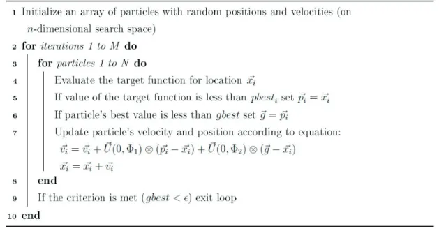
The problem of searching for the absolute effec-tive tensor is nonlinear. In our contribution, the solution is found with a particle-swarm optimiza-tion method (PSO), proposed by Kennedy & Eber-hart (1995). The method is a powerful global op-timization technique which can be applied to the wide range of optimization problems without ne-cessity of its internal parameter tuning (see Poli et al. 2007). This algorithm is often used to find the ef-fective tensor (see Danek et al. 2013, Kozubal 2016). PSO is a stochastic method simulating the behav-iour of animals searching for a food. Particular members of the swarm are described with the par-ticles placed in the n-dimensional solution space. Each particle knows its position (values of solution,
in this case four parts of quaternion) and evalu-ates the target function in its current location. The movement of a single particle through the search space is determined by combining its own cur-rent (xi) and the personal best location (pi) with the global best location (g) and some random pertur-bation. The swarm can be additionally subdivid-ed and then g refers to the best location achieved by a member of the group (in this work we treat a swarm as a fully connected graph). New locations are chosen by adding velocity vi to the coordinate xi (it can be treated as a step-size). The next iteration is calculated after all particles are moved. The initial velocity vi is zero, but before first use it is updated.
The algorithm of canonical PSO optimization is presented in Figure 1 as a pseudo-code (based on Poli et al. 2007).
The update of the particle’s velocity and position use vectors U( , )0 Φi , which are vectors of random
numbers uniformly distributed between [0, Φi],
which are randomly generated at each iteration and for each particle. The operator ⊗ means the com-ponent-wise multiplication. The calculated velocity has to be within the range [−vmax, vmax]. The veloci-ty is usually limited to the highest acceptable value of xi (see Eberhart & Shi 2000). Φ1 and Φ2 are con-striction coefficients limiting particle movements related to the best individual and global positions, respectively.
In our implementation, we used commonly used values of Φi = 2. The algorithm finishes either when the maximum number of iterations or when sufficiently good fit is achieved.
A single value of the target function arises as a result of the rotation of the coordinate system with a given quaternion and the calculation of a specific sum according to the particular symme-try class. Since we use only unit quaternions to pa-rameterise the rotations, we have to normalize the tested quaternions in each iteration.
RESULTS
All analyses in this paper are conducted using the generally anisotropic elasticity tensor (20) obtained by Dewangan & Grechka (2003). The source of 21 elastic stiffness coefficients cij was a multiazimuth, multicomponent VSP data set acquired in New Mexico. The entries are den-sity-scaled so their unit is square kilometre per square second [km2/s2]: C= 7 8195 3 4495 2 5667 2 0 1374 2 0 0558 2 0 1239 3 4495 8 129 . . . ( . ) ( . ) ( . ) . . 55 2 3589 2 0 0812 2 0 0735 2 0 1692 2 5667 2 3589 7 0908 2 0 . ( . ) ( . ) ( . ) . . . ( .- 00092 2 0 0286 2 0 1655 2 0 1374 2 0 0812 2 0 0092 2 1 66 ) ( . ) ( . ) ( . ) ( . ) ( .- ) ( . 336 2 0 0787 2 0 1053 2 0 0558 2 0 0735 2 0 0286 2 0 078 ) ( . ) ( . ) ( . ) ( . ) ( . ) ( . -- 77 2 2 0660 2 0 1517 2 0 1239 2 0 1692 2 0 1655 2 0 1053 ) ( . ) ( . ) ( . ) ( . ) ( . ) ( . ) -22 0 1517( .- ) 2 2 4270( . ) (20) S= ± 0 1656 0 1122 0 1216 2 0 1176 2 0 0774 2 0 0741 0 1122 0 18 . . . ( . ) ( . ) ( . ) . . 662 0 1551 2 0 0797 2 0 1137 2 0 0832 0 1216 0 1551 0 1439 2 0 . ( . ) ( . ) ( . ) . . . ( .00856 2 0 0662 2 0 1010 2 0 1176 2 0 0797 2 0 0856 2 0 071 ) ( . ) ( . ) ( . ) ( . ) ( . ) ( . 44 2 0 0496 2 0 0542 2 0 0774 2 0 1137 2 0 0662 2 0 0496 2 ) ( . ) ( . ) ( . ) ( . ) ( . ) ( . ) (( . ) ( . ) ( . ) ( . ) ( . ) ( . ) ( . 0 0626 2 0 0621 2 0 0741 2 0 0832 2 0 1010 2 0 0542 2 0 00621) 2 0 0802( . ) (21)
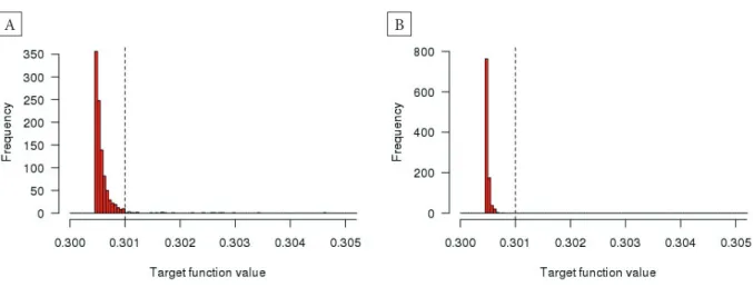
described in the previous section was applied 1000 times in order to obtain the orthotropic ef-fective tensor. Each run produced one quaternion, and, since the optimization algorithm is based on a random search of the solution space, the obtained results differ. However, different quaternions may describe the same rotation of a tensor expressed in several coordinate systems and gives an equal target function, so there are several global minima defining optimal solution for effective tensor (see Equations (23) and (25)). A histogram of the target function values (Fig. 2A) shows that most of the results are close to the global minimum but there are several values diverging from the minimum. It was decided arbitrarily that values right of the vertical line (>0.301) constituting 2.7% of the total number of values should be eliminated from the solutions set. The single optimization (one run of PSO procedure) did not bring a satisfying result and so repeated optimization had to be applied. The stopping criterion for the procedure is defined as follows: if three identical (to the numerical
ac-curacy) quaternions are found, one of them is accepted as a solu-tion. The histogram of values obtained with this approach, which is shown in the right plot of Figure 2, is nar-rower and all the target function values are less than 0.301.
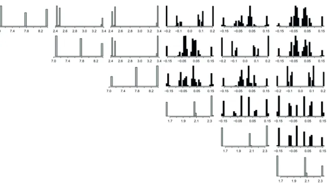
In the crossplots of particular parts of quater-nions obtained with single optimization (Fig. 3), one can see that values are concentrated around certain points.
Circles are black or grey, depending on the tar-get function value. It is clearly visible that in case of some points we do not observe values of target function lower than 0.301. It suggests that these points represent local minima.
For example, by run- ning our procedure, we obtained the following quaternion:
q= -0 00636 0 81548 0 57795. + . i+ . j-0 03050. k (22)
The values are obtained as a result of the meas-urement and inversion of slowness and polariza-tion vectors for the elasticity tensor. Thus, one should treat the tensor as a set of normal dis-tributions of entries, not just their strict values, because the entries are burdened with measure-ment errors. The matrix of standard deviations of tensor entries is given below (Danek & Slawin-ski 2015):
The first tests of our method were conduct-ed using the single tensor (20). The procconduct-edure
Fig. 2. Histograms of the final values of the target function. The described procedure was performed 1000 times to produce the orthotropic effective tensor: A) with a single optimization; B) with the optimization repeated to eliminate diverging values
Fig. 3. Solutions of the procedure for orthotropic class with single optimization (1000 runs). Scatterplot matrix contains all the pairwise crossplots of the particular quaternion parts (Q1–Q4). The tone of points depends on the value of the target function for the solution
The target function for this rotation is equal to 0.30046, and the tensor expressed in transformed coordinate system is as follows:
For the non-zero entries (grey bars), one can clearly see that each entry has three possible values.
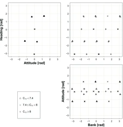
Solutions di-vided into three groups, depend-ing on the value of c11 entry, show easily noticeable patterns in the crossplots of part values (Fig. 5). c11 was used to distinguish 3 forms in which re-sulting tensor is observed (compare Fig. 4) If the values of quaternions are recalculated to Euler an-gles, one can also notice the clear division of the points (Fig. 6). The number of point groups in the quaternion crossplot is doubled, compared to Euler angle crossplots, as two opposite quaternions de-scribe the same set of angles. So- lutions divided with respect to other non-zero entries also give clear patterns but sets of point groups are not al-ways the same.
Since the tensor entries should be treated as distributions, further analyses were conducted with a statistical approach. This means that ten-sors being subject of inversion and rotation were realizations of normal distributions having mean values given with Equation (20) and standard de-viations given with Equation (21) for particular tensor entries.
Three specific tensors from among those 50,000 obtained were additionally marked with a circle, square, or triangle in Figure 7. It confirms the ear-lier observation about the swapping of some entries for tensors in different coordinate systems (e.g. c11,
c22, c33 or c12, c13, c23). The tensors were chosen such that each one is contained in one of three separate groups of solutions shown in Figures 5 and 6. While for non-zero entries pattern of values is clearly visi-ble, we cannot see any rule in zeroed entries. C= -8 3776 3 3626 2 4888 2 0 1136 2 0 0203 2 0 1545 3 3626 7 77 . . . ( . ) ( . ) ( . ) . . 442 2 4267 2 0 0691 2 0 0799 2 0 0244 2 4888 2 4267 7 0810 2 . ( . ) ( . ) ( . ) . . . - - -(( . ) ( . ) ( . ) ( . ) ( . ) ( . ) - -- -0 -0389 2 0 0404 2 0 2068 2 0 1136 2 0 0691 2 0 0389 22 2 0781 2 0 0715 2 0 1479 2 0 0203 2 0 0799 2 0 0404 ( . ) ( . ) ( . ) ( .- ) ( .- ) ( .- ) 22 0 0715 2 1 6500 2 0 0267 2 0 1545 2 0 0244 2 0 2068 2 ( . ) ( . ) ( . ) ( . ) ( . ) ( . ) -- (( .0 1479) 2 0 0267( .- ) 2 2 3315( . ) (23)
The same value of target function was obtained with different quaternion (24) giving tensor (25) as a result of rotation: q=0 01708 0 98520 0 16850. - . i+ . j-0 02621. k (24) C= -7 -7-744 3 3622 2 4262 2 0 0800 2 0 0690 2 0 0248 3 3622 8 37 . . . ( . ) ( . ) ( . ) . . 883 2 4893 2 0 0201 2 01142 2 0 1541 2 4262 2 4893 7 0809 2 0 . ( . ) ( ) ( . ) . . . ( . -00404 2 0 0390 2 0 2068 2 0 0800 2 0 0201 2 0 0404 2 1 6 ) ( . ) ( . ) ( . ) ( . ) ( . ) ( . - -5502 2 0 0720 2 0 0264 2 0 0690 2 01142 2 0 0390 2 0 ) ( . ) ( . ) ( . ) ( ) ( . ) ( . - -- - - 00720 2 2 0779 2 0 1477 2 0 0248 2 0 1541 2 0 2068 2 0 ) ( . ) ( . ) ( . ) ( . ) ( . ) ( -- - - ..0264) 2 0 1477( .- ) 2 2 3311( . ) (25)
Please note, that this is the same tensor de-scribing the same medium but in a different coor-dinate system.
All of the accepted results for many different quaternions (1000) are shown in Figure 4. Please note that when a tensor is expressed in a ent coordinate system, its a entries can have differ-ent values. Nevertheless, this is still exactly the same tensor corresponding with the optimized target function. For entries that were to be zeroed according to the form of the orthotropic tensor (black bars), the distributions of values are ap-proximately symmetrical with the central part about zero. However, none of these entries is equal to zero for any tensor. Additionally, in this exam-ple, the measurement errors of the original ten-sor were not applied in the optimization process. It is also visible that values can be divided into several groups, because the distributions are not continuous.
Fig. 4. Distribution matrix of the tensor entries. Values obtained with the described procedure for one specific orthotropic tensor. Plots represent respective entries in the 6 × 6 matrix (black bars – zeroed entries, grey bars – non-zero entries)
Fig. 5. Scatterplot matrix containing values of particular parts of quaternions for orthotropic class. Points are divided into three groups depending on the value of c11 entry obtained from rotation with specific quaternion
Fig. 6. Scatterplot matrix containing values of Euler angles for orthotropic class. Points are divided into three groups depending on the value of c11 entry obtained through rotation with specific set of angles
Fig. 7. Distribution matrix of the tensor entries for the orthotropic class. 50,000 realizations of tensor generated randomly with normal distributions (instead of exact values of entries) were rotated with quaternions obtained as results of separate optimiza-tions. Entries of three chosen tensors are marked respectively with a circle, triangle and square
The next analyses were conducted for the tetrag-onal symmetry class. In the distributions of the entries obtained as a result of the procedure with the target function specific for tetragonal symme-try (Fig. 8), which were repeated 1000 times, one can notice that the zeroing of respective entries was not as effective as for the orthotropic class. This is visible especially for c45, c46 and c56 entries, where the obtained values are at quite a large dis-tance from zero. The non-zero entries do not show that characteristic pattern known from the orth-otropic class. The pairs of entries expected to be equal have very similar distributions (in respective pairs) and comprise two peaks, each one constitut-ing about half of the values. The other entries have unimodal pseudonormal distributions (differenc-es l(differenc-ess than 0.01). The valu(differenc-es of obtained quatern-ions (Fig. 9) comprise fewer point groups than for the orthotropic class. One group is omitted, be-cause it does not satisfy the criteria to be treated as a global minimum. Here, we can also see the equal partition of quaternions with respect to the c11 en-try value. In the crossplots of Euler angles calcu-lated from mentioned quaternions (Fig. 10), one can see an even more distinct partition for the two
groups. There are only eight sets of angles giving a minimum of the target function.
The distributions obtained as a result of a sepa-rate procedure for 50,000 randomly genea sepa-rated ten-sors (Fig. 11) confirm what we expected after the analysis of the distributions for one specific tensor. Even though we operate with normal distributions (not exact values of entries), there is nearly a zero probability to have c45 entry zeroed. Some entries are apparently unimodal, but it is an effect of the merging of two normal distributions with means differing about 0.1 (c44, c55, c66 – compare Figs. 8 and 11). While entries expected to be equal appear to have nearly identical distributions, we cannot say that entries expected to be zeroed can be equal to zero.
The same analysis conducted for the procedure with the target function specified for the trans-verse isotropic symmetry class shows very similar results (Fig. 12), since a TI class is the subgroup of tetragonal class. The c45value cannot be zero-ed while different conditions describing the TI class seems to be satisfied. The non-zero entries all seems to be unimodal or bimodal with nearly equal modes.
Fig. 8. Distribution matrix of the tensor entries. One specific tensor was rotated with quaternions obtained with 1000 runs of procedure for tetragonal symmetry class (black bars – zeroed, grey bars – non-zero entries)
Fig. 9. Scatterplot matrix containing values of particular parts of quaternions for tetragonal class. Points are divided into three groups depending on the value of the entry obtained from rotation with a specific quaternion
Fig. 10. Scatterplot matrix containing values of Euler angles for tetragonal class. Points are divided into three groups depending on the value of c11 entry obtained through rotation with specific set of angles
Fig. 11. Distribution matrix of the tensor entries for the tetragonal class. 50,000 realizations of tensor generated randomly with normal distributions were rotated with quaternions obtained as results of separate optimizations
Fig. 12. Distribution matrix of the tensor entries for the transverse isotropic class. 50,000 realizations of tensor generated ran-domly with normal distributions were rotated with quaternions obtained as results of separate optimizations
DISCUSSION AND CONCLUSIONS
The described entries zeroing method is a tool to obtain an effective tensor of a certain symmetry from measured generally anisotropic tensor. In this contribution, the orthotropic, tetragonal, and transverse isotropy classes were analysed. Ob-viously, applying the proposed method for other classes is trivial and require only target function modifications similar to the ones used in present-ed examples. Comparison of the obtainpresent-ed results strongly suggests that this tensor belongs to the orthotropic symmetry class. This conclusion is supported by the fact that entry c45 cannot be ze-roed for tetragonal and TI symmetry class (com-pare Figs. 11 and 12). Please note, that in error-free case original tensor cannot be considered as an orthotropic (see Fig. 4).In this work, an algorithm was tested for three symmetry classes. The choice of the classes was based on a priori information about the medium being measured in the original field experiment. As the isotropic effective tensor is calculated ana-lytically and is independent of the orientation, the described method does not apply to this class.
For the orthotropic class, there are the same possible values of the respective entries (i.e. c11,
c22, c33), but recorded with a different frequency. The interpretation of this phenomenon is that the same tensor is expressed in three different coordi-nate systems rotated by π/2 (please see Fig. 6 and compare Danek et al. 2013).
The obtained results can be compared with the effects of previous methods based on the op-timization of the Frobenius distance. A compari-son of the respective entries of the effective tensor belonging to a given class can be performed in-stantaneously. When comparing the orientations described with the quaternion or set of Euler an-gles, one should remember that in distance-based methods the coordinate system of the effective ten-sor is rotated to the coordinate system of the meas-ured tensor, while in the entries zeroing method the transformation is done in reverse direction.
In general, the obtained results are in agree-ment with those obtained by Danek et al. (2013). In all analysed cases, very similar solutions can be found for both methods. In some cases, e.g. tetragonal class, the entry zeroing method is not
sensitive enough to provide all expected solutions (only two possible values of the bank angle with π step, while Danek et al. have found eight possible orientations with π/4 step). Nevertheless, we con-sider this result satisfactory.
The proposed method may be used to replace or complement the existing method of describing the symmetry class and orientation of the medi-um based on the elasticity tensor measured in situ with vertical seismic profiling, with its less com-plex target function and process of optimization being an advantage of the described method.
This research was partially supported by the National Science Centre of Poland under contract No. DEC-2013/11/B/ST10/0472 and by AGH Uni-versity of Science and Technology, Faculty of Geol-ogy, Geophysics and Environmental Protection as a part of the statutory project No. 11.11.140.613.
REFERENCES
Bona A., Bucataru I. & Slawinski M.A., 2004. Characteriza-tion of Elasticity-Tensor Symmetries Using SU(2). Jour-nal of Elasticity, 75, 3, 267–289.
Danek T., Kochetov M. & Slawinski M.A., 2013. Uncertain-ty analysis of effective elasticiUncertain-ty tensors using quatern-ion-based global optimization and Monte-Carlo meth-od. The Quarterly Journal of Mechanics and Applied Mathematics, 66, 2, 253–272.
Danek T. & Slawinski M.A., 2015. On choosing effective elasticity tensors using a Monte-Carlo Method. Acta Ge-ophysica, 63, 1, 45–61.
Dewangan P. & Grechka V., 2003. Inversion of multicompo-nent, multiazimuth, walkaway VSP data for the stiffness tensor. Geophysics, 68, 3, 1022–1031.
Diner C., Kochetov M. & Slawinski M.A., 2011. On choos-ing effective symmetry classes for elasticity tensors. The Quarterly Journal of Mechanics and Applied Mathemat-ics, 64, 1, 57–74.
Eberhart R.C. & Shi Y., 2000. Comparing inertia weights and constriction factors in particle swarm optimization. [in:] Proceedings of the 2000 Congress on Evolutionary Computation: CEC00: July 16–19, 2000, La Jolla Marriott Hotel, La Jolla, California, USA, IEEE Service Center, 84–88.
Forte S. & Vianello M., 1996. Symmetry Classes for Elastici-ty Tensor. Journal of ElasticiElastici-ty, 43, 2, 81–108.
Gierlach B. & Danek T., 2017. Obtaining orthotropic elas-ticity tensor using entries zeroing method. [in:] EGU European Geosciences Union: general assembly 2017: Vienna, Austria, 23–28 April 2017, Geophysical Re-search Abstracts, 19, [on-line:] http://meetingorganiz-er.copernicus.org/EGU2017/EGU2017-438.pdf [access: 10.06.2018].
Hamilton W.R., 1844. On a new species of imaginary quan-tities connected with a theory of quaternions. Proceed-ings of the Royal Irish Academy, 2, 424–434.
Kennedy J. & Eberhart R.C., 1995. Particle swarm optimiza-tion. [in:] 1995 IEEE International Conference on Neural Networks: proceedings, the University of Western Austral-ia, Perth, Western AustralAustral-ia, 27 November-1 December 1995, IEEE, 1942–1948.
Kochetov M. & Slawinski M.A., 2009. On obtaining effec-tive orthotropic elasticity tensors. The Quarterly Journal of Mechanics and Applied Mathematics, 62, 2, 149–166. Kozubal A., 2016. Global and local stochastic
optimiza-tion in effective elasticity tensors evaluaoptimiza-tion. [in:] 15th
International Conference on Geoinformatics – Theoreti-cal and Applied Aspects (Geoinformatics 2016): Proceed-ings of a meeting held 10–13 May 2016, Kiev, Ukraine, EAGE, 454.
Poli R., Kennedy J. & Blackwell T., 2007. Particle swarm opti-mization – An overview. Swarm Intelligence, 1, 1, 33–57. Shoemake K., 1985. Animating rotation with quatern-ion curves. ACM SIGGRAPH computer graphics, 19, 3, 245–254.
Slawinski M.A., 2010. Waves and Rays in Elastic Continua. World Scientific, Singapore.
Slawinski M.A., 2016. Wavefronts and rays in seismology. An-swers to unasked questions. World Scientific, Singapore.