Title Relevance-Redundancy Dominance: a threshold-free approach to filter-based feature selection
Author(s) Browne, David; Manna, Carlo; Prestwich, Steven Editor(s) Greene, Derek
MacNamee, Brian Ross, Robert Publication date 2016-09
Original citation Browne, D., Manna, C. and Prestwich, S. (2016) 'Relevance-Redundancy Dominance: a threshold-free approach to filter-based feature selection', in Greene, D., MacNamee, B. and Ross, R. (eds.) Proceedings of the 24th Irish Conference on Artificial Intelligence and Cognitive Science 2016, Dublin, Ireland, 20-21 September. CEUR Workshop Proceedings, 1751, pp. 227-238
Type of publication Conference item Link to publisher's
version http://ceur-ws.org/Vol-1751/Access to the full text of the published version may require a subscription.
Rights © 2016, David Browne, Carlo Manna and Steven Prestwich. http://ceur-ws.org/
Item downloaded
from http://hdl.handle.net/10468/4461
Downloaded on 2018-08-23T20:02:09Z
Relevance-Redundancy Dominance: a
Threshold-Free Approach to Filter-Based
Feature Selection
D. Browne, C. Manna, and S. D. Prestwich
{david.browne,carlo.manna,steven.prestwich}@insight-centre.org Insight Centre for Data Analytics, University College Cork, Ireland
Abstract. Feature selection is used to select a subset of relevant features in machine learning, and is vital for simplification, improving efficiency and reducing overfitting. In filter-based feature selection, a statistic such as correlation or entropy is computed between each feature and the target variable to evaluate feature relevance. A relevance threshold is typically used to limit the set of selected features, and features can also be removed based on redundancy (similarity to other features). Some methods are de-signed for use with a specific statistic or certain types of data. We present a new filter-based method called Relevance-Redundancy Dominance that applies to mixed data types, can use a wide variety of statistics, and does not require a threshold. Finally, we provide preliminary results, through extensive numerical experiments on public credit datasets.
1
Introduction
Many real-world applications deal with high-dimensional data, andfeature selec-tionis a well-known and important class of methods for reducing dimensionality. Feature selection reduces data size, and improves learning accuracy and compre-hensibility. The methods are usually categorized as filter,wrapper or embedded [7]. Filter methods rely on the general characteristics of the training data to select features with independence of any predictor, wrapper methods involve optimizing a predictor as part of the selection process, and embedded methods try to combine the advantages of both. In this paper we focus on filter-based methods, which are considered to be most scalable to big data. Furthermore, we focus on univariate methods which evaluate (and usually rank) single features, asmultivariate methods are computationally expensive.
We propose a new filter-based feature selection method called Relevance-Redundancy Dominance (RRD) feature selection, with a simple feature elimi-nation strategy based on relevance and redundancy. It can be applied to mixed data types, can use a wide variety of statistics, requires no threshold for choos-ing a feature subset, and in experiments outperforms published methods on four credit datasets.
2
Related Work
Feature selection strategies based on filter methods have received attention from many researchers in statistics and machine learning. Their advantages are that they are fast, independent of the classifier/predictor method, scalable and easy to interpret.
The RELIEF algorithm [12] estimates the quality of attributes according to how well their values distinguish between instances that are near to each other. It can deal with discrete and continuous features but was initially limited to two-class problems. An extension, ReliefF [13], not only deals with multiclass problems but is also more robust and capable of dealing with incomplete and noisy data. The Relief family of methods are especially attractive because they may be applied in all situations, have low bias, include interaction among features and may capture local dependencies that other methods miss. However, they select features based only on relevance and do not remove redundant features.
Correlation-based Feature Selection (CFS) [8] is a simple filter algorithm that ranks feature subsets according to a correlation-based heuristic evaluation function. The bias of the evaluation function is toward subsets that contain features that are highly correlated with the class and uncorrelated with each other. Irrelevant features should be ignored because they will have low correlation with the class. Redundant features should be screened out as they will be highly correlated with one or more of the remaining features. Moreover, there exists an improved CFS version called Fast Correlated-Based Filter (FCBF) method [27] based on symmetrical uncertainty (SU) [20], which is defined as the ratio between the information gain (IG) and the entropy (H) of two features. This method was designed for high-dimensionality data and has been shown to be effective in removing both irrelevant and redundant features (although it fails to take into consideration interactions between features). The INTERACT algorithm [28] uses the same goodness measure as the FCBF filter [20], but also includes the consistency contribution (c-contribution). The c-contribution of a feature indicates how significantly the elimination of that feature will affect consistency. The algorithm consists of two major parts. In the first part, the features are ranked in descending order based on their SU values. In the second part, features are evaluated one by one starting from the end of the ranked feature list. If the c-contribution of a feature is less than a given threshold the feature is removed, otherwise it is selected.
Finally, the Minimum Redundancy-Maximum Relevance (MRMR) [15] is a heuristic framework which minimizes redundancy, using a series of measures of relevance and redundancy to select promising features for both continuous and discrete data sets. Particularly, for discrete variables it applies Mutual Informa-tion, while for continuous variables it mainly uses the F-test and correlation.
3
The proposed method
RRD is a univariate filter-based feature selection method, which can use any suitable statistic to select agoodsubset of features in a dataset. The statistic can
be symmetric (s(f, f0)≡s(f0, f) for example correlation or mutual information) or asymmetric (for example Goodman and Kruskal’sλ[6]).
Given a binary statistics, featuresf ∈F and a target variablet, the RRD method works as follows. As in other methods, the features are ranked for rele-vance usings: f is more relevant than f0 ifs(f, t)> s(f0, t). We shall say that
f dominates f0 ifs(f, t)> s(f0, t) ands(f, f0)> s(f0, t). We shall also say that
f0 is redundant if it is dominated by f and f is not dominated by any other feature. RRD selects all non-redundant features.
This leads to the feature selection method shown in Algorithm 1. First we precompute the statistics xf t = s(f, t) between each feature f and the target variablet, and initialise the set of selected features to the empty set∅. Then we select the feature ˆf ∈F with greatest relevancexf tˆ, generate the setRoff ∈F
that are made redundant by ˆf, addR to S, and remove R∪ {fˆ} from F. The last few steps are repeated untilF is empty, then we return the setS of selected features.
Algorithm 1RRD Feature Selection Algorithm given featuresF and targett
∀f∈F xf t←s(f, t) S← ∅ whileF 6=∅ ˆ f←arg maxf∈Fxf t R← {f|f∈F∧s( ˆf , f)> xf t} F←F\(R∪ {fˆ}) S←S∪ {fˆ} returnS
Note that Algorithm 1 typically does not compute alls-values between fea-tures (for example a full correlation matrix). This is because after a feature has been removed fromF no further statistics on it need be computed. This means that it will often compute fewer statistics than (say) the MRMR method of [15], though in the worst case it computes the same number. It is possible to construct datasets for which RRD removes no features at all, or removes all but one, but in practice we find that it usually generates a small subset of features.
Finally, it should be pointed out that RRD assumes that we can compute statistics(x, y) for allx, y∈F∪{t}. Thus before we can apply RRD, if the target and/or features have mixed types (numerical, ordinal, nominal) they must be first preprocessed so that they are all of the same type. This preprocessing is detailed in the next section.
4
Experiments on real datasets
We performed extensive experiments on 4 datasets using 12 statistics, 7 dis-cretization methods, and 3 classifiers.
Datasets
RRD was evaluated on 4 credit datasets from the UCI Machine Learning Reposi-tory [14], each with a binary target variable. We decided to evaluate our method thoroughly on one type of data, rather than partially on several data types, though we are also working on other datasets. Feature selection for credit data has been the subject of several recent papers.
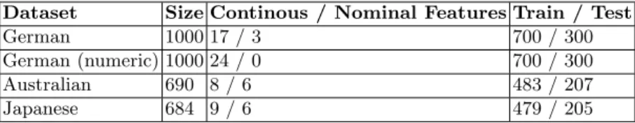
Table 1 provides an overview of the 4 datasets used in the numerical experi-ments. The German dataset has 3 continuous features, 4 ordinal features and 13 nominal features, while the numerical version of the German dataset has 24 con-tinuous features. Both the Australian and Japanese datasets have 6 concon-tinuous features, the Australian dataset also has 8 nominal features, and the Japanese dataset has 9 nominal features. These are popular datasets for evaluating clas-sification and feature selection methods, especially where credit scoring is the research topic.
Table 1.Credit datasets
Dataset Size Continous / Nominal Features Train / Test
German 1000 17 / 3 700 / 300
German (numeric) 1000 24 / 0 700 / 300
Australian 690 8 / 6 483 / 207
Japanese 684 9 / 6 479 / 205
Discretization
In classification problems we are typically faced with mixed-type features and a nominal (often binary) target, so we may apply preprocessing. In this work we transform all data to nominal form via discretization, which groups continuous feature values into bins. We used 7 binning methods including 2 supervised (Chi2 and Extended Chi2which are based on information theory) and 5 unsupervised. The unsupervised binning methods were: equal frequency and equal width, in which the cube root of the number of samples was used to determine the num-ber of bins;k-means clustering, where the value of kwas determined using the
pn
2 method, the elbow method, and the floor value of the natural log of the
continuous data.
It should be noted that if the dataset being analysed has all continuous numerical features and either a binary or continuous target variable, RRD can use statistics such as Spearman’s correlation to reduce the number of features.
This removes the need for discretization, which simplifies RRD and improves its computational efficency.
Statistics
RRD is capable of analysing all types of data, including hybrid data, using any suitable statistic whether they are use correlation criteria (such as Pearson’s correlation coefficient) or information-based (such as mutual information) [1, 18, 22–25, 27]. In this paper 12 different statistics were used to select the optimal subsets for the credit datasets.
Classifiers
We used 3 classifiers: Logistic Regression, Random Forests and Naive Bayes. A Logistic Regression model can be used as a classifier when the target variable is binary. It uses a sigmoid function to calculate to which class a test subject belongs. Random Forests [2] is an ensemble learning algorithm. Naive Bayes classifiers are based on Bayes’ Theorem. We chose these three methods because they are popular yet distinct. All three can handle mixed data types, but often perform better when continuous features are transformed into nominal form [5].
Cross-validation
We used stratified 100-fold Monte Carlo cross-validation with 70%/30% train-ing/testing splitting of the data, as follows: (i) randomly split the data set samples into 70% training set and 30% testing set; (ii) using only the training set, create bins for the discretization method; (iii) run RRD on the discretized training set to find the optimal features; (iv) using the training set subset, build the predictor model (e.g. Naive Bayes); (v) select the same features in the test set as RRD selected in the training set; (vi) using the bin cut-points found in step (ii) discretize the test set; (vii) evaluate the predictor model built in step (iv) using the test set, which has been kept completely isolated from the training set, and finally (viii) repeat steps (i) to (vii)k times (in this paper k = 100). Average prediction accuracy and number of selected features, along with their corresponding standard deviations, are reported in each case.
Results
The best results for each classifier and statistic are shown in Tables 3–5 in the Appendix (results for the numerical German dataset are omitted due to lack of space). These can be compared to published results from various papers using both new and well established filter feature selection methods, shown in Table 2.
The best RRD result on the German dataset was 76.13% ± 1.76% with 13.3±0.46 selected features, using Messenger & Mandell’sΘ [19] andk-means
discretization, which outperformed the majority of the other methods, and was on par with the best, the selective Bayesian classifier of [21] with 76.21% and 6 selected features. The worst result was 70.99% ± 1.67% with Goodman & Kruskal λusing Naive Bayes as the classifier andk-means elbow discretization method.
On the numerical German dataset our best result was 75.38%±1.69% us-ing Messenger & Mandell’s Θ and equal width discretization, with 11.99 ±0.1 selected features. This is beaten by the SVM + Grid search + F-score method of [10] with 77.50% and approximately 20 selected features, so our accuracy is slightly worse but with 8 fewer features selected. The worst result was 70.32% ±3.34% with Somers’δ using Naive Bayes as the classifier andk-means elbow discretization method.
On the Australian dataset Goodman & Kruskal’sλ with Chi2 binning and
the Naive Bayes classifier was the most accurate with 86.29%±1.97%. This was better than the result from Chen [3] using DT + SVM. The worst result was 84.54% ±2.53% with Mutual InformationI using Naive Bayes as the classifier and equal frequency discretization method.
On the Japanese dataset Somers’δ with equal frequency discretization was the most accurate: 87.04%±1.94% and 3.95±0.39 selected features. This beats the ECMBF method of Jiang [11] with 2 selected features and 85.45%. The worst result was 85.68% ±2.18% with Mutual InformationI, Naive Bayes and equal width discretization.
In summary, the best results were found by Random Forests, the most robust statistics were Messenger & Mandell’sΘand Cramer’sφc, and the best binning methods were generally the unsupervised k-means and equal width discretiza-tion. Overall RRD performed excellently, selecting 6%– 65% of features while achieving very competitive accuracies compared to published results.
5
Conclusion
We proposed a new filter-based feature selection algorithm called RRD with several advantages over existing methods: it can use a variety of statistics; it can handle combinations of nominal, ordinal and numerical data; it takes both relevance and redundancy into account; and it automatically decides how many features to select without the need for a threshold or cut-off (though one could be added if necessary). In experiments on credit data it outperformed published methods.
In future work we shall test RRD further, especially investigating its scal-ability to big data. We shall also investigate whether it continues to select an appropriate number of features on other datasets. An early result in this direc-tion uses the Musk dataset from the UCI Machine Learning Repository [14], which involves predicting whether a molecule is a musk or not. It has 166 nu-meric features, a binary target variable, and 6598 samples. RRD’s best result so far is 95.58% ±0.44% with 9.5±1.18 selected features, using Cramer’s φc and equal frequency discretization. This beats the published result of Lou [16]
of 92.4% with 6 features using HSMB algorithm, and is similar to the best result of [26] with 96.35%±0.51% with 25 selected features using FCBF-P.
Acknowledgments
This work was supported in part by Science Foundation Ireland (SFI) under Grant Number SFI/12/RC/2289, and was aided by the availability of bench-marks in the UCI Machine Learning Repository [14].
References
1. A. Agresti. Categorical Data Analysis. John Wiley and Sons, pp. 57–59, 2002. 2. L. Breiman and J. Friedman. Classification and Regression Trees. Chapman and
Hall, New York, USA, 1984.
3. F. Chen, F. Li. Combination of Feature Selection Approaches With SVM in Credit Scoring.Expert Systems with Applications.37:4902–4909, 2010.
4. P. O’Dea, J. Griffith, C. O’Riordan. Combining Feature Selection and Neural Net-works for Solving Classiciation Problems.In: Proceedings of The Irish Conference on Artifical Intelligence & Cognitive Science,pp. 157–166, 2001.
5. J. Dougherty, R. Kohavi, M. Sahami. Supervised and unsupervised discretization of continuous features.In: Machine Learning: Proceedings of the Twelfth Interna-tional Conference,pp. 194–202, 1995.
6. L. A. Goodman and W. H. Kruskal. Measures of Association for Cross Classifica-tions. New York: Springer-Verlag (contains articles appearing in J. Amer. Statist. Assoc. in 1954, 1959, 1963, 1972), 1979.
7. I. Guyon. Feature Extraction: Foundations and Applications, vol. 207, Springer, 2006.
8. M. A. Hall. Correlation-based Feature Selection for Machine Learning.PhD thesis., Department of Computer Science, Waikato University, New Zealand, 1999. 9. M. A. Hall, L. A. Smith. Feature Subset Selection: A Correlation Based Filter
Approach. University of Waikato, Hamilton, New Zealand.
10. C. Haung, M. Chen, C. Wang. Credit Scoring With a Data Mining Approach Based on Support Vector Machines.Expert Systems with Applications.33:847–856, 2007. 11. S. Jiang, L. Wang. Efficient Feature Selection Based on Correlation Measure Be-tween Continuous and Discrete Features.Information Processing Letters 116(2), 2016.
12. K. Kira, L. Rendell. A Practical Approach to Feature Selection.In: Proceedings of the Ninth International Conference on Machine Learning,pp. 249–256, 1992. 13. I. Kononenko. Estimating Attributes: Analysis and Extensions of RELIEF. In:
Bergadano, F., De Raedt, L. (eds.), Machine Learning: ECML-94, LNCS vol. 784, pp. 171–182, Springer, Heidelberg, 1994.
14. M. Lichman. UCI Machine Learning Repository. University of California, Irvine, School of Information and Computer Sciences, 2013, http://archive.ics.uci.edu/ml 15. H. C. Peng, F. Long, C. Ding. Feature Selection Based on Mutual Information: Criteria of Max-Dependency, Max-Relevance, and Min-Redundancy.IEEE Trans-actions on Pattern Analysis and Machine Intelligence 27(8):1226–1238, 2005. 16. Q. Lou and Z. Obradovicl. Feature selection by approximating the Markov Blanket
in a kernel-induced space.In:Europe Conference on Artificial Intelligence,pp. 797– 802, 2010.
17. H. Lui, R. Setiono. A Probabilistic Approach to Feature Selection - A Filter Solu-tion.. In Machine Learning: Proceedings of the Thirteenth International Confer-ence on Machine Learning,Morgan Kaufmann, 1996.
18. Z. Masoumeh and K. R. Seeja. Feature Extraction or Feature Selection for Text Classification: A Case Study on Phishing Email Detection. Information Engineer-ing and Electronic Business, 2015.
19. R. C. Messenger and L. M. Mandell. A Modal Search Technique for Predictive Nominal Scale Multivariate Analysis.Journal of the American Statistical Associa-tion 67, 1972.
20. W. H. Press, B. P. Flannery, S. A. Teukolsky, W. T. Vetterling. Numerical Recipes in C. Cambridge University Press, Cambridge, 1988.
21. C. A. Ratanamahatana, D. Gunopulos. Scaling Up the Naive Bayesian Classifier: Using Decision Trees for Feature Selection.. In Machine Learning: Proceedings of Workshop Data Cleaning and Preprocessing (DCAP ’02) at IEEE Int’l Conf. Data Mining,, 2002.
22. A. Stuart. The Estimation and Comparison of Strengths of Association in Contin-gency Tables.Biometrika 40:105–110, 1953.
23. H. Theil. Statistical Decomposition Analysis. Amsterdam: North-Holland Publish-ing Company, 1972.
24. A. A. Tschuprow. Principles of the Mathematical Theory of Correlation. W. Hodge & Co., 1939.
25. B. Wu and L. Zhang. Feature Selection via Cramer’s V-Test Discretization for Remote-Sensing Image Classification. IEEE Transactions on Geoscience and Re-mote Sensing 52(5), 2014.
26. L. Yu, H. Liu. Efficiently handling feature redundancy in high-dimensional data.
In:The Ninth ACM SIGKDD International Conference on Knowledge Discovery and Data Mining (KDD-03),pp. 685–690, 2003.
27. L. Yu, H. Liu. Feature Selection for High-Dimensional Data: A Fast Correlation-Based Filter Solution.In: ICML, Proceedings of The Twentieth International Con-ference on Machine Learning,pp. 856–863, 2003.
28. Z. Zhao, H. Liu. Searching for Interacting Features. In: IJCAI, Proceedings of International Joint Conference on Artificial Intelligence, pp. 1156–1161, 2007.
Table 2.Feature selection results from related work
dataset selected accuracy algorithm paper
German 6 76.21% SBC [21] 6 76.13% ABC [21] 7 75.85% NN [4] 4 74.38% NB ECMBF [11] 20 74.32% NB Full-set [11] 14 73.87% NB Consistency [11] 4 73.76% NB FCBF [11] 3 73.24% NB CFS [11] 4 72.18% C4.5 ECMBF [11] 3 71.47% C4.5 CFS [11] 4 71.32% C4.5 FCBF [11] 14 71.26% C4.5 Consistency [11] 20 71.26% C4.5 Full-set [11]
German 20.4 77.50% SVM + Grid search+ F-Score [10] (numerical) 12 76.70% F-score + SVM [3] 12 76.10% LDA + SVM [3] 12 75.60% RST + SVM [3] 24 75.40% Full-set + SVM [3] 12 73.70% DT + SVM [3] Australian 7 86.52% LDA + SVM [3] 7 86.29% DT + SVM [3] 2 85.79% C4.5 ECMBF [11] 2 85.79% NB ECMBF [11] 7 85.22% RST + SVM [3] 7 85.10% F-score + SVM [3] 5 84.80% C4.5 - LV F [17] 1 84.65% IB1-CFS [9] 14 84.34% Full-set + SVM [3]
7.6 84.20% SVM + Grid search+ F-Score [10]
14 83.91% C4.5 Full-set [11] 13 83.83% C4.5 Consistency [11] 1 83.78% Naive-CFS [9] 7 83.49% C4.5 FCBF [11] 7 83.32% C4.5 CFS [11] 5 80.30% ID3 - LV F [17] 14 76.09% NB Full-set [11] 7 75.32% NB CFS [11] 13 74.89% NB Consistency [11] 7 73.57% NB FCBF [11] Japanese 2 85.45% C4.5 ECMBF [11] 15 85.83% C4.5 Full-set [11] 7 85.28% C4.5 CFS [11] 2 84.94% NB ECMBF [11] 6 84.77% C4.5 FCBF [11] 13 84.68% C4.5 Consistency [11] 15 78.13% NB Full-set [11] 13 75.32% NB Consistency [11] 6 75.23% NB FCBF [11] 7 74.81% NB CFS [11]
Table 3.German credit dataset RRD results
Classifier Statistic Selected Accuracy Discretization Logistic Messenger & Mandell’sΘ 13.27±0.45 75.32±2.12 Equal Width Model Cramer’sφc 5.18±0.78 74.64±2.33k-means Elbow
Stuart’sτc 5.19±0.9 73.92±2.02k-means Elbow
Tschuprow’sT 3.59±0.55 73.7±2.1 k-means Elbow Theil’sU 3.61±0.75 73.58±2.11k-means Elbow Mutual InformationI 2.17±0.38 72.73±2.06k-means Elbow Goodman & Kruskal’sγ 5.05±0.9 72.69±1.84 Chi2 Contingency CoefficientC 2.26±0.52 72.62±1.9 k-means Elbow Pearson’sχ2 2.24±0.51 72.62±1.89k-means Elbow Somers’δ 4.32±0.74 71.69±2.14 Chi2 Goodman & Kruskal’sλ 1.12±0.33 71.6±1.44 Floor (ln) Naive Messenger & Mandell’sΘ 13.27±0.45 75.66±2.32 k-means Bayes Cramer’sφc 5.22±0.73 74.44±2.1 k-means Elbow
Stuart’sτc 5.18±0.94 74.31±2.27k-means Elbow
Tschuprow’sT 3.6±0.64 73.74±2.16k-means Elbow Theil’sU 3.56±0.74 73.65±2.28k-means Elbow Mutual InformationI 2.21±0.43 72.54±2.38k-means Elbow Pearson’sχ2 2.2±0.43 72.49±2.3 k-means Elbow Contingency CoefficientC 2.24±0.45 72.46±2.33k-means Elbow Goodman & Kruskal’sγ 5.09±1.04 71.99±2.34 Chi2 Somers’δ 4.2±0.71 71.67±2.49 Chi2 Goodman & Kruskal’sλ 2.07±0.36 70.99±1.67k-means Elbow Random Messenger & Mandell’sΘ 13.3±0.46 76.13±1.76 k-means Forest Cramer’sφc 5.12±0.74 73.74±2.35k-means Elbow
Theil’sU 3.55±0.73 73.22±2.39k-means Elbow Tschuprow’sT 3.51±0.56 73.18±2.29k-means Elbow Stuart’sτc 5.16±0.88 72.56±2.43k-means Elbow
Mutual InformationI 2.22±0.44 72.07±1.8 k-means Elbow Pearson’sχ2 2.23±0.49 71.97±1.7 k-means Elbow Contingency CoefficientC 2.27±0.51 71.95±1.71k-means Elbow Somers’δ 4.77±0.79 71.7±2.29 Extended Chi2 Goodman & Kruskal’sλ 2.08±0.34 71.66±1.44k-means Elbow Goodman & Kruskal’sγ 5.05±1.08 71.65±2.07 Extended Chi2
Table 4.Australian credit dataset RRD results
Classifier Statistic Selected Accuracy Discretization Logistic Goodman & Kruskal’sλ 7.62±0.92 85.98±2.14 Extended Chi2 Model Tschuprow’sT 6±0.79 85.86±2.07 Extended Chi2 Cramer’sφc 5.62±0.81 85.83±2.09 Extended Chi2
Goodman & Kruskal’sγ 5.32±0.74 85.78±1.99 k-means Stuart’sτc 5.33±0.55 85.78±1.78 Equal Freq
Messenger & Mandell’sΘ 8±0 85.74±1.87 Chi2 Theil’sU 4.88±0.79 85.54±2.01 Extended Chi2 Somers’δ 6.08±0.84 85.37±1.97 Extended Chi2 Mutual InformationI 4.28±0.9 85.29±1.88 Extended Chi2 Pearson’sχ2 4±0.85 85.27±1.91 Extended Chi2 Contingency CoefficientC4.07±0.84 85.26±1.9 Extended Chi2 Naive Somers’δ 3.94±0.28 85.9±2.19 Equal Freq Bayes Tschuprow’sT 5.38±0.68 85.53±2.46 Equal Freq Messenger & Mandell’sΘ 5.4±0.49 85.47±2.68 Equal Width Cramer’sφc 6.21±0.73 85.34±2.62 Equal Freq
Goodman & Kruskal’sγ 4.99±0.54 85.33±2.3 Equal Freq Theil’sU 5.45±0.66 85.31±2.46 Equal Freq Goodman & Kruskal’sλ 7.91±0.6 85.08±2.21 Equal Freq Stuart’sτc 5.24±0.57 84.98±2.47 Equal Freq
Contingency CoefficientC3.05±0.46 84.63±2.53 Equal Freq Pearson’sχ2 3.05±0.46 84.63±2.53 Equal Freq Mutual InformationI 3.28±0.71 84.54±2.53 Equal Freq Random Goodman & Kruskal’sλ 8.58±0.55 86.29±1.97 Chi2 Forest Messenger & Mandell’sΘ 8.05±0.22 86.09±1.87 k-means
Cramer’sφc 7.4±0.55 86.06±1.83 Chi2
Somers’δ 6.09±0.87 85.71±2.09 Extended Chi2 Stuart’sτc 6.49±0.8 85.69±1.92 Floor (ln)
Tschuprow’sT 5.2±0.71 85.57±2.05 Floor (ln) Goodman & Kruskal’sγ 5.63±0.77 85.49±2.1 k-means Elbow Contingency CoefficientC 2.04±0.2 85.34±2.15 k-means Pearson’sχ2 2.04±0.2 85.34±2.15 k-means Mutual InformationI 2.13±0.34 85.33±2.15 k-means Theil’sU 2.97±0.36 85.06±2.13 Equal Width
Table 5.Japanese credit dataset RRD results
Classifier Statistic Selected Accuracy Discretization Logistic Goodman & Kruskal’sλ 7.43±0.9 86.56±2.07 Extended Chi2 Model Stuart’sτc 5.79±0.82 86.55±2.12 Extended Chi2
Tschuprow’sT 6.17±0.88 86.44±2.1 Extended Chi2 Cramer’sφc 6.28±0.87 86.42±2.23 Equal Freq
Goodman & Kruskal’sγ 5.43±0.98 86.31±2.01 Extended Chi2 Messenger & Mandell’sΘ 7.98±0.14 86.24±2.25 Chi2 Theil’sU 5.29±0.91 86.24±2.19 Extended Chi2 Mutual InformationI 4.64±0.96 86.18±2 Extended Chi2 Somers’δ 6±0.91 86.14±2.05 Extended Chi2 Contingency CoefficientC4.53±0.89 86.1±2.06 Extended Chi2 Pearson’sχ2 4.45±0.91 86.1±2.03 Extended Chi2 Naive Somers’δ 3.95±0.39 87.04±1.94 Equal Freq Bayes Cramer’sφc 6.2±0.77 86.47±2.02 Equal Freq
Messenger & Mandell’sΘ 5.28±0.45 86.45±1.96 Equal Width Theil’sU 5.52±0.63 86.33±2.09 Equal Freq Goodman & Kruskal’sγ 4.65±0.73 86.32±1.89 Equal Freq Tschuprow’sT 5.49±0.88 86.22±2.09 Equal Freq Stuart’sτc 5.43±0.86 86.12±1.91 Equal Freq
Goodman & Kruskal’sλ 7.55±0.61 85.86±1.94 Equal Freq Contingency CoefficientC3.03±0.17 85.76±1.94 Equal Width Pearson’sχ2 3.03±0.17 85.71±1.92 Equal Width Mutual InformationI 3.06±0.28 85.68±2.18 Equal Width Random Messenger & Mandell’sΘ 8.13±0.34 86.58±2.14 k-means Forest Somers’δ 3.97±0.3 86.52±2.2 Chi2
Goodman & Kruskal’sλ 8.16±0.39 86.51±1.97 Chi2 Tschuprow’sT 6.19±0.94 86.49±2.22 Chi2 Cramer’sφc 7.65±0.48 86.41±1.88 Chi2
Stuart’sτc 5.97±0.73 86.37±2.18 k-means
Goodman & Kruskal’sγ 5.18±0.99 86.3±2.06 k-means Contingency CoefficientC2.06±0.24 86.13±1.98 k-means Pearson’sχ2 2.06±0.24 86.13±1.98 k-means Mutual InformationI 2.16±0.37 86.12±2.01 k-means Theil’sU 4.57±0.71 85.95±1.85k-means Elbow