Efficient OLAP Operations in Spatial Data Warehouses

Efficient OLAP Operations in Spatial Data Warehouses

Department of Computer Science Hong Kong University of Science and Technology

Clear Water Bay, Hong Kong

{dimitris, kalnis, zhangjun, taoyf}@cs.ust.hk

Abstract. Spatial databases store information about the position of individual objects in space. In many applications however, such as traffic supervision or mobile communications, only summarized data, like the number of cars in an area or phones serviced by a cell, is required. Although this information can be obtained from transactional spatial databases, its computation is expensive, rendering online processing inapplicable. Driven by the non-spatial paradigm, spatial data warehouses can be constructed to accelerate spatial OLAP operations. In this paper we consider the star-schema and we focus on the spatial dimensions. Unlike the non-spatial case, the groupings and the hierarchies can be numerous and unknown at design time, therefore the well-known materialization techniques are not directly applicable. In order to address this problem, we construct an ad-hoc grouping hierarchy based on the spatial index at the finest spatial granularity. We incorporate this hierarchy in the lattice model and present efficient methods to process arbitrary aggregations. We finally extend our technique to moving objects by employing incremental update methods.

1

Introduction

Data warehouses are collections of historical, summarized, non-volatile data, which are accumulated from transactional databases. They are optimized for On-Line Analytical Processing (OLAP) [CCS93] and have proven to be valuable on assisting decision-making. The data in a warehouse are conceptually modeled as hyper-cubes [GBLP96] where each dimension represents some business perspective, like products and stores, and the cube cells contain a measure, such as sales.

Recently, the popularity of spatial information, such as maps created from satellite images and the utilization of telemetry systems, has created repositories of huge amounts of data which need to be efficiently analyzed. In analogy to the non-spatial case, a spatial data warehouse can be considered, which supports OLAP operations on both spatial and non-spatial data.

Han et. al.[HSK98; SHK00] were the first ones to propose a framework for spatial data warehouses. They considered an extension of the star-schema [K96] in which the cube dimensions can be both spatial and non-spatial and the measures are regions in space, in addition to numerical data. They focus on the spatial measures and propose a method for selecting spatial objects for materialization. The idea is similar to the

algorithm of [HRU96], the main difference being the finer granularity of the selected objects. In [ZTH99], an I/O efficient method is presented for merging spatial objects. The method is applied on the computation of aggregations for spatial measures.

In this paper we concentrate on the spatial dimensions. The fact that differentiates the spatial attributes from the non-spatial ones is that there is little or no a-priori knowledge about the grouping hierarchy. The user, in addition to some predefined regions, may request groupings based on maps which are computed on the fly, or may be arbitrarily created (e.g. an arbitrary grid in a selected window). Therefore the well-known pre-aggregation methods [HRU96; G97; GM99; SDN98] which are used to enhance the system performance under OLAP operations, cannot be applied.

Motivated by this fact, we propose a method which combines spatial indexing with the pre-aggregated results. We built a spatial index on the objects of the finer granularity in the spatial dimension and use the groupings of the index to define a hierarchy. We incorporate this implicit hierarchy to the lattice model of Harinarayan et. al, [HRU96] to select the appropriate aggregations for materialization. We study several algorithms for spatial aggregation and we propose a method which traverses the index in a breadth-first manner in order to compute efficiently group-by queries. Finally we employ incremental update techniques and show that our method is also applicable for moving objects.

Storing aggregated results in the index for non-spatial warehouses has been proposed by Jurgens and Lenz [JL98]. Lazaridis and Mehrotra [LM01] use a similar structure for on-line computation of approximated results which are progressivly refined. Yang and Widom [YW01] also employ an aggregation tree for incremental maintenance of temporal aggregates. None of these papers considers spatial objects.

There are numerous applications that benefit from our method. Throughout this paper we use an example of a decision support system for traffic control in a city. Some of the queries that can be answered efficiently are “which is the total number of cars inside every district”, or “find the road with the highest traffic in a 2km radius around every hospital”. One could also use data from other sources, like a map which groups the city based on the pollution levels, and group the traffic data based on the regions of the pollution map. Other application domains include network traffic control and congestion prevention systems for cellular communications, meteorological applications, etc.

The rest of the paper is organized as follows: Section 2 provides a brief overview of OLAP and a motivating example followed throughout the paper. Section 3 proposes the aR-tree which keeps aggregated information organized according to the spatial dimensions. Section 4 describes algorithms for query processing and Section 5 discusses update issues. Section 6 evaluates the approach experimentally, while Section 7 concludes the paper with future directions and potential applications.

2

Related Work and Motivating Example

In this work we assume that the multi-dimensional data are mapped on a relational database using a star schema [K96]. Let D1, D2, …, Dn be the dimensions (i.e. business perspectives) of the database, such as Product, Store and Time. Let M be the

measure of interest; Sales for example. Each Di stores details about the dimension, while M is stored in a fact table F. Each tuple of F contains the measure plus pointers (i.e. foreign keys) to the dimension tables (Figure 1a).

There are O(2n) possible group-by queries for a data warehouse with n dimensional attributes. A detailed group-by query can be used to answer more abstract aggregations. [HRU96] introduce the search lattice L, which represents the interdependencies among group-bys. L is a directed graph whose nodes represent group-by queries. There is an edge from node uito node uj, if uican be used to answer

uj(see Figure 1b). For instance the aggregated results per product (node P) can be computed from the results of product/store (node PS) or product/time (node PT).

The aggregation functions are divided into three classes [GPLP96]: distributive, algebraic and holistic. Distributive aggregate functions can be computed by partitioning their input into disjoint sets, aggregating each set individually and obtaining the final result by further aggregating the partial results. COUNT, SUM, MIN and MAX belong to this category. Algebraic aggregate functions can be expressed as a scalar function of distributive functions. AVERAGE, for example, is an algebraic function since it can be expressed as SUM / COUNT. Holistic aggregate functions (e.g. MEDIAN) cannot be computed by dividing the input into parts. The proposed techniques can be applied for distributive and algebraic functions.

It is common in OLAP applications, to include hierarchies for several dimensions: for instance, various types of products for which we want aggregated statistical information. Another example is time where at the finer granularity data are grouped by day, but the user may ask queries which involve grouping by week, month or year. In order to accelerate such queries, all or some [BPT97; HRU96; G97; GM99; SDN98] of these results can be precalculated and materialized. Extending the example to spatial dimensions, we could have pre-aggregated results for stores in specific regions of interest, e.g., cities, states, countries and so on. The motivation for this work comes from the fact that in the spatial case, these hierarchies are often not known in advance. In the example of Figure 1, for instance, assume that users ask for sales of stores in several query windows, which differ depending on their interests.

As a more realistic application, consider a traffic supervision system that monitors the positions of cars in a city and the road traffic (for the following examples we assume that a car does not necessarily lie on a road segment, e.g., it can be in a parking lot). The goal of such a system can be: "find the road segments with the heaviest traffic near the center" or, given a medical emergency, "which is the hospital that can be reached faster given the current traffic situation". In both cases, it is

FACT TABLE Product_ID Store_ID Time_ID Sales PRODUCT Product_ID Description Color Shape STORE Store_ID Location TIME Time_ID Day Month Quarter Year PCT PS PT ST P S T all

(a) The star schema (b) The data-cube lattice Fig. 1. A data warehouse schema with dimensions Product, Customer and Time

statistical information, i.e., the number of cars, rather than their ids that is important. Furthermore, the extraction of this information can be time consuming. Consider that the positions of the cars are stored in an R-tree RC, and the extents of the line segments in a tree RR. Answering a query such as "give me the traffic for every road segment in an area of 1km radius around each hospital" would require a spatial join between RCand RR. The same system could also be used to answer queries involving fire emergencies, in which case the areas of interest would be around fire departments (police stations and so on).

Even if the join result is pre-computed and stored for each segment, the existence of spatial conditions (area of 1km radius around each hospital), calls for some spatial indexing technique. Driven by the data warehouse paradigm, a spatial data warehouse can be constructed [HSK98; SHK00] to answer analytical queries more efficiently. A spatial warehouse can be represented by a star schema: Diis the set of dimensions of interest and F the fact table which contains the aggregated results for the spatial dimension at the finest granularity (in this case the number of cars per road segment). For ease of understanding assume that there is no other dimension except the spatial one (we will extend our model to many dimensions in a following section). In the rest of the paper we describe a data structure and associated query processing mechanisms for retrieval of spatial aggregated results.

3

The Aggregation R-Tree Structure

Let SD be a spatial database and C a spatial relation that stores the positions of cars. C is indexed by an R-Tree RC. Let R be a spatial relation that stores all the objects that belong to the spatial dimension (i.e. roads), at the finest granularity. R is also indexed by an R-Tree RR. Let AG(·) be the aggregation function. Without loss of generality, we will assume that AG(·) is COUNT, although any non-holistic function can be used.

The aggregation R-Tree (aR-tree) is an R-Tree which stores for each minimum bounding rectangle (MBR), the value of the aggregation function for all the objects that are enclosed by the MBR. The aR-tree is built on the finest granularity objects of the spatial dimension, therefore its structure is similar to that of RR(the trees can be different due to the smaller fanout of the aR-tree). Figure 2 depicts an aR-tree which

a2,3 a3,1 a5,2 a1,0 a4,4 A1,6 A2,4 aR 0 1 a5 a2 a3 a1 a4 A1 A2 + + + + + + +++ + q q1q2

indexes a set of five road segments, r1… r5, whose MBRs are a1… a5respectively. There are three cars on road r2, therefore there is an entry (a2,3) in the leaf node of the aR-tree. Moving one level up, MBR A1contains three roads, r2, r3and r5. The total number of cars in these roads is six; therefore there is an entry (A1, 6) at level one of the aR-tree. The general concept can be applied to different types of queries; for instance, instead of keeping aggregated results of joins the aR-tree could store such results for window queries. Furthermore we could employ the same idea to other data partitioning or space partitioning data structures (e.g., Quadtrees).

In the rest of the paper, we make the distinction between an aR-tree node Xiand its

entries Xi,1,.., Xi,CPi, (where CPi≤CP is the capacity of Xi) which correspond to MBRs included in Xi. Xi,k.ref points to the corresponding node Xk at the next (lower) level. For instance, at level 1 of the first tree, the entries of the root are A1and A2, which point to nodes at level 0. The pre-aggregated result for each entry is denoted by Xi,k.agr. Each node Xialso has a pointer Xi.next, which points to the next node Xi+1at the same level (we will justify the need for this pointer below).

It is straightforward to extend the above definition to handle multiple aggregate functions. Instead of storing one result in each entry of the tree, we store a list of results for all the necessary functions. In our example, if the maximum number of cars in each road is also required, the entry for A1will be (A1, 6, 3) since there are 3 cars on road r2. In this way, the aR-tree can also handle algebraic aggregate functions. If, for instance, we need the average number of cars in each road segment covered by a node, in addition to the total number of cars we need to store the number of road segments covered by the node.

The value of AG(⋅) for all leaf level entries (i.e., road segments) in the aR-tree can be computed by an R-tree spatial join algorithm [BKS93] if both datasets are indexed by R-trees, or by employing specialized spatial join indexes [R91]. Nodes can then be constructed in a bottom-up fashion by using information of the lower levels. An important property of the aR-tree is that every object at level l-1, belongs to exactly one MBR at level l. This fact allows us to store partial results and aggregate them in a further step to get more general results, which correspond to the roll-up operation in OLAP terminology. For instance, the total number of cars in all roads of Figure 2 is calculated by adding the materialized results for A1and A2, i.e. 6 plus 4. Assuming that the many-to-one property didn’t hold, such operations wouldn’t be possible because some object could be counted multiple times.

Lemma 1: The aR-tree defines a hierarchy among MBRs that forms a data cube

lattice1_[HRU96].

Proof: (sketch) Let Elbe the set of materialized results for all entries of all nodes of the aR-tree at level l, i.e. El= {Xi,j.agr,∀Xiin level l,∀j∈[1, CPi]}. Following the notation of [HRU96], we say that Ei ≤ Ej if Ei can be answered by Ej. From the previous discussion it is obvious that an aggregation query El can be answered by further aggregating the materialized results of El-1. Therefore El+1≤El∀l∈[0, h-1], where h is the height of the tree. Eh contains only one member, which is the

1 _{Strictly speaking, a hierarchy is a lattice [TM75] if there is a least upper bound and a greatest}

lower bound for every two elements according to the≤ ordering. Here we adopt the term “lattice” since it is standard in the OLAP literature.

aggregated result of all objects. Thus, the aR-tree defines a hierarchy, which is a data cube lattice, since there is:

1. An operator≤which imposes a partial order to the sets El. 2. A top element E0upon which every set Elis dependant.

Figure 3 depicts the lattice which corresponds to the aR-tree of the previous example. Notice that, in order to be compatible with the standard OLAP notation, the order of materialized results is inversed compared to the tree (i.e., E0, which corresponds to the leaf level is at the top of the lattice).

E0= (3, 1, 2, 0, 4)≡(AG(a2), AG(a3), AG(a5), AG(a1), AG(a4))

E1= (6, 4)≡(AG(a2, a3, a5), AG(a1, a4))

E0

E1

E2 E

2= (10)≡(AG(a2, a3, a5, a1, a4))≡all

Fig. 3. The lattice for the aR-tree of Figure 2

By incorporating the aR-tree to the lattice framework, we can take advantage of the extensive work that exists for non-spatial data warehouses, both on modeling and efficient implementation. We highlight some of these issues below:

• Multiple dimensions: Until now we only considered the spatial dimension (recall that we model the n-D space that the spatial data belongs to, as one dimension in the warehouse). Assume that there are k dimensions represented by the lattices L1,

…, Lk respectively, in addition to the spatial dimension which is represented by lattice L0. The data cube lattice is defined as the product of L0⋅L1⋅…⋅Lk (see [HRU96] for details). In Figure 4a, there is the spatial dimension from the aR-tree of Figure 2, and a non-spatial dimension Ct→all which models vehicle types (i.e. truck, bus, small car, etc). Figure 4b depicts the resulting 2-D data cube lattice. The node E0Ctfor example corresponds to the query that returns the number of vehicles in each road grouped by their type. At the physical level, the entries of the aR-tree must be extended to support multiple dimensions. In addition to the previous information, there is a pointer to a multidimensional array which contains the aggregated values for the whole domain of the other dimensions. It is also possible for a spatial data warehouse to have more than one spatial dimension. In our example, assume that for each car, we know its starting position (e.g. the address of the owner) and we want to group the cars both by the starting and the current

E0 E1 all Ct all E0Ct E1Ct E0 Ct E1 all

(a) A spatial and a non-spatial dimension (b) The resulting data cube lattice Fig. 4. A data cube which includes both a spatial and a non-spatial dimension

position (e.g. in road r1there are 3 cars which came from the east part of the city and 2 cars from the west part). The current position of each car is independent of its starting position; therefore we can model this problem by two orthogonal dimensions on the data cube. For each dimension we build a separate aR-tree. • View selection: Although the materialization technique accelerates the OLAP

operations, usually it is not practical to materialize all the possible aggregations because of storage and/or update cost constraints. A number of methods [HRU96; G97; GM99; SDN98] have been proposed which select a set of views to materialize based on a benefit metric. The lattice framework allows us to employ similar techniques for spatial dimensions. Selecting a view in the spatial case corresponds to selecting a set El (i.e., a level) of the aR-tree for materialization. Since some of the intermediate levels may not be materialized, we must assure that the structure of the tree is preserved. Assume that the set Elis not selected. Let Xi,j be an entry at level l+1 and Xk, …, Xk+m be the nodes of level l-1 which are enclosed by the MBR of Xi,j. Then Xi,j.ref is changed to point to Xkand we create a linked list which contains all nodes from Xkto Xk+m. This is repeated for all entries of level l+1. In Figure 5, a four-level tree is depicted, where only levels 0 and 3 are materialized. Observe that the first entry of level 3 points to the first node of level 0, and there is a linked list that connects this node to the following three that contain objects which are enclosed by the MBR of the entry at level 3. The remaining part of the tree is constructed in the same way.

E0 E1

E2

E3

Fig. 5. Partial materialization of the aR-tree

• Multiple spatial hierarchies: We stated above that the aR-tree is beneficial since the groupings at the spatial dimension are usually unknown. However, in some applications there may exist some default groupings in addition to the ad-hoc ones. In our running example there may be a grouping of the city roads based on the areas of responsibility of each police station, and another grouping for the areas that are covered by each fire station. Such cases are modeled as dimensions with multiple hierarchies. If the aggregations for the default groupings are materialized, the queries that involve these groupings will run faster than if the aR-tree were accessed. Ad-hoc groupings, however, still need the aR-tree. The multiple hierarchy lattice can be the input of the view selection algorithm. Therefore, a combination of default groupings and levels of the aR-tree are selected, based on the distribution and the cost of the queries.

• Spatial measures: In the previous discussion we dealt only with numeric measures. The aR-tree structure can be extended to support spatial measures (see Han et. al [HSK98; SHK00]). In this case, Xi,j.agr is substituted by a pointer to the aggregated object. Both spatial and numeric measures can coexist in the same aR-tree.

4

Query Processing

Lets start with a simple query of the form: "find the total number of cars on all road segments inside a query window". As an example consider Figure 2 and window q. Using only the transactional database, we should perform the query directly on the base relations, i.e., the cars and the road segments. As an alternative we could pre-compute and store in a table the number of cars per road segment, in which case a sequential scan of the table is required; each road segment is compared with q, and if q contains the segment, its aggregated value is updated. For roads that partially overlap the query window, we may need to perform the joins with the base relations in order to compute the actual results. For instance, although we store that there are four cars in segment a4, we do not know which of these cars is inside the window. Alternatively, if precision is not vital, we could assume uniformity and estimate the number of cars depending on the percentage of the road segment inside the query window.

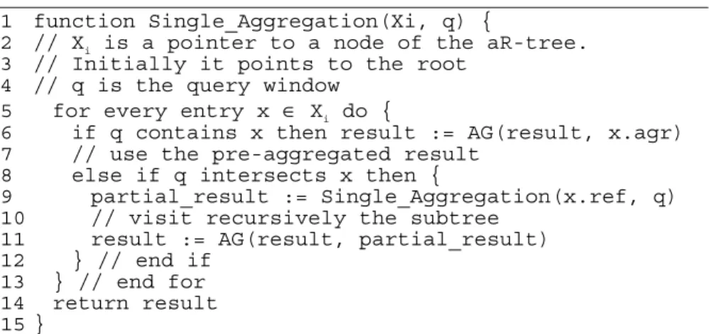
Using aR-trees, the processing of this query starts from the root of the tree and proceeds recursively to the leaves. For all entries one of the following three conditions may hold:

• The entry is disjoint with the query window; thus, the corresponding node cannot contain any cars contributing to the answer and is not retrieved.

• The entry is inside the query window (e.g., A1 in Figure 2) in which case all aggregate information is stored with the entry and the corresponding node does not need to be accessed.

• The entry partially overlaps the query window in which case the corresponding node must be recursively followed.

For leaf entries that partially overlap the query window, we could either use estimations (as described above), or compute the actual results using the base tables. The pseudo-code for aggregated window queries is shown in Figure 6.

The algorithm is similar to the window-query algorithm for common R-Trees. There is, however, a fundamental difference. For common window queries, if the query window is very large the use of the index does not pay off and the optimizer uses sequential search on the MBRs of the objects. For aggregate queries, on the other hand, there are two cases:

1. The query window q is large; then many nodes in the intermediate levels of the aR-tree will be contained in q so the pre-calculated results are used and we avoid visiting the individual objects.

2. The query window is small. In this case the aR-tree is used as a spatial index, allowing us to select the qualifying objects.

Now assume that there are multiple query windows and the goal is “for each query window, find the total number of cars on all road segments inside it”. We define Q as a set of k query windows, i.e. Q = {q1, q2, ..., qk}. Each window qidefines a grouping region where the aggregation function AG(⋅) must be evaluated. In the example of Figure 2, the plane is divided in two windows, q1and q2. There are 6 and 4 cars in the

q1 and q2 region respectively, therefore the result of the above query contains two tuples: {(q1, 6), (q2, 4)}. Note that the union of all grouping windows doesn’t

necessarily cover the entire space, and the grouping windows may intersect with each other.

If there are no pre-aggregated results available, this query can be modeled and processed as a multiway spatial join [MP99]. In particular, the sets to be joined are the cars, the roads and the query windows. Similar to the case of single window, if we have pre-aggregated results in the form of a table, each row is compared with every window qi, and if qicontains the segment, its aggregated value is updated. Partial containment can be handled again by estimations or computation using the base relations.

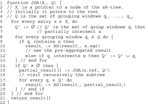
In the presence of aR-trees, the query is modeled as a pairwise spatial join between the set of query windows and the aR-tree. Any algorithm for joining an indexed with an non-indexed set (query windows) could be used [LR94; PRS99; MP99]. Actually since in most cases the number of windows is expected to be rather small, we can assume that this set can fit in memory. Under this assumption, we can traverse the aR-tree in a top-down fashion, and recursively follow only entries that partially intersect some window. We call this algorithm Join Group Aggregation (JGA); the pseudo-code is illustrated in Figure 7.

Both types of queries can be easily extended to retrieve aggregated results at the finer resolution, i.e., "for each road segment inside the query window, find the number of cars". In this case, even nodes contained inside the window(s) should be traversed all the way to the leaves, in order to find the qualifying road segments; thus, the aR-tree acts as a spatial index on the fact table.

1 function Single_Aggregation(Xi, q) {

2 // Xi is a pointer to a node of the aR-tree.

3 // Initially it points to the root 4 // q is the query window

5 for every entry x ∈ Xi do {

6 if q contains x then result := AG(result, x.agr) 7 // use the pre-aggregated result

8 else if q intersects x then {

9 partial_result := Single_Aggregation(x.ref, q) 10 // visit recursively the subtree

11 result := AG(result, partial_result) 12 } // end if

13 } // end for 14 return result 15 }

5

Updates

When the data in the spatial database changes, the updates must be propagated to the data warehouse. Here, we assume that the dimensions do not change (i.e. the map of roads is not altered), which is true for most applications. Therefore we only consider changes to the raw data (the positions of the cars in our example). For efficiency reasons, the updates of the warehouse should not occur during its normal operation. It is common practice [GM95; MQM97] that the warehouse goes off-line in regular intervals, when the updates are propagated to it and any required reorganization takes place. The off-line period should be minimized; in practice, mainly because of this constraint it is impossible to materialize all the possible aggregations [GM99].

The naïve updating method is to recalculate the whole aR-tree. The cost of this operation is unacceptably high, since it involves a spatial join between the raw data and the dimensions. Better performance can be achieved by incrementally updating [GMS93] the aR-Tree. The idea is that we keep a recordδC of the changes in C. Such information is usually available in the log file of the database. In our example, δC contains the set of cars that change position. For each of these cars,δC stores a tuple containing the car id together with its old and new position. The size of δC is expected to be smaller than C. The aR-tree can then be updated as follows: For each tuple inδC, perform a search in the aR-tree to find the road with the old position of the car. Update the aggregated value (in our case decrease the car counter by one) and

1 function JGA(Xi, Q) {

2 // Xi is a pointer to a node of the aR-tree.

3 // Initially it points to the root

4 // Q is the set of grouping windows q₁, ..., q_|Q| 5 for every entry x ∈ Xi do

6 Q' := ∅ // Q' is the set of group windows q_i that

7 // partially intersect x

8 for every grouping window qi ∈ Q do {

9 if q_i contains x then

10 result_i := AG(result_i, x.agr) 11 // use the pre-aggregated result

12 else if q_i intersects x then Q' := Q' ∪ q_i 13 } // end for

14 if Q' ≠ ∅ then {

15 partial_result[] := JGA(x.ref, Q’) 16 // visit recursively the subtree 17 for every qi ∈ Q' do

18 result_i := AG(result_i, partial_result_i) 19 } // end if

20 } // end for 21 return result[] 22 }

propagate the change to the higher levels of the tree. Then search the aR-tree for the road of the new position of the car. Update the aggregation and propagate the changes. We call this algorithm Individual Incremental Update (IIU). Observe that the procedure that propagates a change in the leaf nodes to the higher levels of the tree, essentially visits the same nodes with the search procedure. The reason we don’t update the intermediate levels while searching, is that an object may not belong to any leaf node of the tree (e.g., a car may be in a parking lot). This complication, however, does not necessarily increase the I/Os. The searching algorithm sends a hint to the cache to pin all the pages (i.e. nodes) which are visited. Therefore, these pages are not evicted from the cache until search and all necessary updates are complete. In most cases the height of the aR-tree does not exceed 4-5 levels, thus no more that 5 pages need to be pinned.

The above algorithm has the following drawback: if k cars enter a road rm, then the corresponding entry amin the aR-tree must be accessed k times by following the same path in the tree. It is obvious that only one access is needed, given the aggregated information for the objects inδC. In order to overcome this problem, we employ an algorithm, called Batch Incremental Update (BIU) which is similar to [MQM97]. In a pre-processing step, BIU performs a spatial join betweenδC and the set of roads. The result of the join is a relationδF which contains the set of roads that need to change their aggregated value, together with the difference of the value. For instance, if 3 cars enter the road rmand 5 leave it, there will be a tuple (rm, -2) inδF. Note that during the computation ofδF, the aR-tree is still on-line. In the second step of the algorithm, the aR-tree goes off-line and the update is performed as in IIU, by using the data of

δF.

By implementing an efficient incremental update method, the aR-tree can support a wide range of real-time applications. The traffic supervision system for example, can be extended to store both spatial and temporal information about each car (i.e. the position of every car at different timestamps). Visualization tools use this information to create real-time maps about traffic congestion. Clearly, the size of the spatio-temporal database is even larger than the spatial one; therefore it is impractical to answer such queries without pre-aggregated results. As another example, in cellular telecommunications it is also important to have real-time summarized information, in order to adjust the capacity of each cell in a way that maximizes the utilization of the network.

6

Experiments

In this section, we evaluate the proposed methods by simulating the scenario of the traffic supervision system that was discussed in the previous sections. We employed the TIGER/Line 1990 dataset which contains around 130,000 line segments corresponding to roads of California (Figure 8a). Using this map, we generated the positions of the cars in the following way: We randomly selected 5,000 seed points which were located on roads. For each seed point pi, we generated a cluster whose centroid was pi and contained 250 points (i.e. car positions) with Gaussian distribution; therefore the total number of cars was 1,25M. By using this method to

generate the points we attempted to reflect the fact that cars tend to be clustered around areas with dense road network.

We implemented the aR-tree, by modifying an R*-Tree [BKSS90] implementation. We set the page size to 1,024 bytes resulting to a fan-out of 42 for the aR-tree. In our experiments, the aR-tree contained 4 levels. In all experiments, we compared the various methods in terms of node accesses.

First, we evaluated the performance of the aR-tree for single window aggregation queries. At a pre-processing step, we populated the aggregated values in the aR-tree by joining the roads with the cars datasets. We generated a set of workloads each consisting of 200 window queries with the same size. In the first workload every window covers 0.0001% of the total space, in the second one 0.001% and so on. The distribution of the queries follows the distribution of the roads on the map, thus avoiding meaningless queries that fall into empty areas (e.g., the sea). Figure 8b depicts an example workload where the size of each query is set to 1% of the total space.

We employed the Single_Aggregation algorithm of Figure 6 for querying the aR-tree and we compared it against two alternatives: (i) querying the raw data: We executed the queries by performing a select-and-join operation on the roads and the cars datasets, using the algorithm of Brinkhoff et.al. [BKS93] (both datasets are indexed by R*-Trees). (ii) querying an R-tree-indexed fact table: Recall that the fact table F contains tuples of the form (MBRroad, agr_value). We processed the query by performing a window search on RR (the roads R-Tree) and then reading the aggregated values from F for the qualifying tuples. The results are summarized in Figure 9, where we draw the average number of node accesses for the 200 queries of each workload. For small windows (less than 0.01% of the total space) the aR-tree doesn’t provide any benefit compared to the indexed fact table approach. The reason is that since the queries are small, they do not contain intermediate entries of the aR-tree; therefore, the Single_Aggregation algorithm has to access the leaf nodes and the aR-tree behaves as a spatial index. For larger windows, however, the aR-tree performs considerably better; for windows covering 10% of the space, the fact-table approach is an order of magnitude worse.

The cost of accessing the raw data is much higher in all cases and the difference from the other methods increases for larger windows. An interesting observation is

(a) Road segments of California (b) A workload of 200 queries Fig. 8. Dataset and query set visualization

that the cost for both the raw-data and the fact-table method, increases monotonically with the window size; a larger window covers more roads and both of these methods always need to access the roads inside the query window. The aR-tree, however, stops searching when an intermediate node is contained in the query window. By increasing the window size, more intermediate nodes satisfy this requirement, therefore the number of node accesses increases at a slower rate. Beyond a threshold size (i.e. 10% of the space) we observe that the number of node accesses starts to decrease. In the extreme case that the window covers the whole space, only one access is required, since all the objects are covered by the entries of the root.

The afore-mentioned methods compute the exact number of cars in a query window. This means that if the query partially intersects the MBR of a road segment, the fact-table and the aR-tree approach, need to access the base relations in order to determine how many cars are in the part of the road inside the window. We do this for fairness of comparison, since the raw-data method computes the exact values by default. In a real environment, however, the interpretation of a window query may vary. A user may be interested just in cars which belong to roads that are intersected by a query window (the cars themselves may be outside), or only in the roads that are totally covered by the window. In these cases, all the information is already summarized. Furthermore, a simple estimation for the marginal road segments (using their overlap with the query window) may be sufficient for many applications. Figure 9 includes the cost of computing an estimated answer using the aR-tree. The trend is the same as for computing the exact answer; however the actual cost is always lower due to not accessing the base relations.

In the next set of experiments we tested the performance of the aR-tree for multiple-window aggregation queries. We compared four methods: (i) aR-Tree (JGA) is the algorithm of Figure 7, which utilizes the aR-tree structure. (ii) aR-tree (single queries): We modeled a multiple-window aggregation as a set of single-window queries and used the Single_Aggregation algorithm of Figure 6. (iii) Fact-table (join):

aR-tree Fact table Raw data aR-tree Estimation

1e+0 1e+1 1e+2 1e+3 1e+4 1e+5 0.0001 0.001 0.01 0.1 1 10 100

Query Window Area (%)

No de Ac ce ss es

In this method, only the indexed fact tableFis materialized and we perform a spatial

join betweenFusing its spatial indexRRand the set of query windows, which fits in

memory. (iv)Fact-table (single queries): Again, the multiple-window aggregation is

modeled as a set of single-window aggregations which run against the indexed fact table. We do not present any results for a raw-data approach because the cost is much higher than the other methods.

The set of query windows was generated as follows: Each query consists of n×n

tiles which represent query windows and is placed randomly on the map. Each tile

covers 1% of the total space. We variednfrom 1 to 5, thus covering 1% to 25% of the

total space. Like the previous experiment, workloads of 200 multiple queries were generated and we calculated the average query cost in terms of nodes accessed. The results are presented in Figure 10a. As expected, the fact-table-based approaches are outperformed by the aR-tree methods, since the former ones always access data at the finest granularity (i.e. roads). Notice that JGA algorithm outperforms the naïve method of executing many single queries and the gap between these methods

aR-tree (JGA) aR-tree (single queries) Fact table (join) Fact table (single queries)

0 500 1000 1500 2000 2500 3000 3500 4000 4500 1 4 9 16 25

Query Window Area (%)

N o d e A cce ss es

(a) 1, 2×2, 3×3, 4×4 and 5×5 groups of windows. Each window occupies 1% of the total space

0 1000 2000 3000 4000 5000 6000 4 16 64 Number of partitions N o d e a cces se s

(b) The whole space is divided in 2×2, 4×4 and 8×8 query windows Fig. 10. Multiple window aggregation queries

increases with the number of windows. This happens because as the number of windows increases, there is a higher chance that two or more of them intersect the same entries of the aR-tree. JGA takes advantage of this fact, by visiting the corresponding nodes only once for all windows; therefore it saves many node accesses.

In Figure 10b, we consider the case that the union of all query windows covers the

entire space. We divided the workspace in 2×2, 4×4 and 8×8 regions and we run the

same algorithms. The trend for the aR-tree based techniques is similar to the previous diagram. The fact-table approaches were around one order of magnitude worse. The cost for the fact-table-join method was constant for any number of partitions, since the algorithm essentially visits the entries for all roads. This behavior corresponds to the worst case of the JGA algorithm, i.e. there is a large number of very small query windows which cover the entire space. In the same way, the fact-table-single-queries method, corresponds to the worst case of the aR-tree-single-queries algorithm.

The last set of experiments focuses on the update methods for the aR-tree. In order to generate some realistic movement of cars, we used the GSTD utility [TSN99]. GSTD is a data generator available on the web, which is used for creating

spatiotemporal data under various distributions. The output of the program is the δC

file which contains the ids of the cars that have moved and their old and new position.

Agility is the number of moving cars over their total number. Note that the total number of cars on all roads is not preserved after an update as new cars may enter or exit the road network. Figure 11 compares Individual Incremental Update (IIU) with Batch Incremental Update (BIU) as a function of the object agility. The measurement

only considers the node accesses that happen when the aR-tree isoff-line; therefore,

the node accesses for the pre-processing step of BIU are not counted. BIU is more than 2 orders of magnitude better than IIU; this fact justifies the suitability of BIU for real-time applications. We do not present the results for re-building the aR-tree from scratch, since it is much worse than both incremental methods.

Batch Incremental Update Indivial Incremental Update

1e+3 1e+4 1e+5 1e+6 0 0.1 0.2 0.3 0.4 0.5 0.6 0.7 0.8 0.9 1 Agility Nod e Ac ces se s

7

Conclusions

In this paper we dealt with the problem of providing OLAP operations in spatial data warehouses. Such warehouses should support spatial dimensions, i.e. allow the user to execute aggregation queries in groups, based on the position of objects in space. Although there exist well-known pre-aggregation techniques for non-spatial warehouses, which aim to accelerate such queries, they cannot be applied in the spatial case because the groupings and the hierarchies among them are unknown at the design time. Such problems arise in many real-life applications. Throughout the paper we presented an example of a traffic supervision system; other applications include decision support systems for cellular networks, weather forecasting, etc.

Motivated by this fact, we propose a data structure, named aR-tree, which combines a spatial index with the materialization technique. The aR-tree is an R-Tree which stores for each MBR, the value of the aggregation function for all objects that are enclosed by it. Therefore, an aggregation query does not need to access all the enclosed objects, since part of the answer is found in the intermediate nodes of the tree. The aR-tree also defines an ad-hoc hierarchy of the objects, which allows us to construct a hierarchy-lattice and take advantage of the extensive work that has been done on the lattice framework (e.g. supporting non-spatial dimension, view selection, etc). We have demonstrated the applicability of the aR-tree through a set of initial experiments that attempt to simulate real life situations.

Currently, we are working towards extending our structure for spatio-temporal applications. In such applications, we need to perform aggregations on both the spatial and temporal dimensions, as well as their combination. Therefore, it is necessary to keep information about the history of the objects. The temporal dimension also complicates the semantics of the aggregation queries, since some distributive functions (e.g. COUNT) behave as holistic ones, unless some additional information is stored. Nevertheless spatio-temporal OLAP is a very promising area both from the theoretical and practical point of view.

In terms of applications it will enable analysts to identify certain motion and traffic patterns which cannot be easily found by using the raw data. Furthermore, although the datasets may have high agility, the summarized information may not change significantly. For instance, although there exist numerous moving cars (or mobile phone users) in urban areas during peak hours, the summarized data may remain constant for long intervals as the number of cars entering is similar to that exiting the area. Given the fact, that in these applications summarized information is more important than the actual data, we believe that efficient multi-version extensions of the aR-tree (or similar structures) are more crucial than typical spatio-temporal access methods.

Acknowledgments

This work was supported by grants HKUST 6070/00E and HKUST 6090/99E from Hong Kong RGC

References

[BKS93] Brinkhoff, T., Kriegel, H.P., Seeger B. Efficient Processing of Spatial Joins Using R-trees. ACM SIGMOD, 1993.

[BKSS90] Beckmann, N., Kriegel, H.P. Schneider, R., Seeger, B. The R*-tree: an Efficient and Robust Access Method for Points and Rectangles. ACM SIGMOD, 1990.

[BPT97] Baralis E., Paraboschi S., Teniente E. Materialized View Selection in a Multidimensional Database. VLDB, 1997.

[CCS93] Codd E., Codd S., Salley C. Providing OLAP (On-Line Analytical Processing) to User-Analysts: An IT Mandate. Technical Report, 1993, available at http://www.arborsoft.com/essbase/ wht_ppr/coddps.zip

[G97] Gupta H. Selection of Views to Materialize in a Data Warehouse. ICDT, 1997. [GBLP96] Gray J., Bosworth A., Layman A., Pirahesh H. Data Cube: a Relational

Aggregation Operator Generalizing Group-by, Cross-tabs and Subtotals. ICDE, 1996.

[GM95] Gupta A., Mumick I. Maintenance of Materialized Views: Problems, Techniques, and Applications. Data Engineering Bulletin, June 1995.

[GM99] Gupta H., Mumick I. Selection of Views to Materialize Under a Maintenance-Time Constraint. ICDT, 1999.

[GMS93] Gupta A., Mumick I., Subrahmanian V. Maintaining Views Incrementally. ACM

SIGMOD, 1993.

[HRU96] Harinarayan V., Rajaraman A., Ullman J. Implementing Data Cubes Efficiently.

ACM SIGMOD, 1996.

[HSK98] Han J., Stefanovic N., Koperski K. Selective Materialization: An Efficient Method for Spatial Data Cube Construction. PAKDD, 1998.

[JL98] Jurgens M., Lenz H.J. The Ra*-tree: An improved R-tree with Materialized Data for

Supporting Range Queries on OLAP-Data. DEXA Workshop, 1998. [K96] Kimball R. The Data Warehouse Toolkit. John Wiley, 1996.

[LM01] Lazaridis I., Mehrotra S. Progressive Approximate Aggregate Queries with a Multi-Resolution Tree Structure. ACM SIGMOD, 2001.

[LR94] Lo, M-L., Ravishankar, C.V. Spatial Joins Using Seeded Trees. ACM SIGMOD, 1994.

[MP99] Mamoulis, N, Papadias, D., Integration of Spatial Join Algorithms for Processing Multiple Inputs. ACM SIGMOD, 1999.

[MQM97] Mumick I., Quass D., Mumick B. Maintenance of Data Cubes and Summary Tables in a Warehouse. ACM SIGMOD, 1997.

[PRS99] Papadopoulos, A.N., Rigaux P., Scholl, M. A Performance Evaluation of Spatial Join Processing Strategies. SSD, 1999.

[R91] Rotem, D. Spatial Join Indices. IEEE ICDE, 1991.

[SDN98] Shukla A., Deshpande P., Naughton J. Materialized View Selection for Multidimensional Datasets, VLDB, 1998.

[SHK00] Stefanovic N., Han J., Koperski K. Object-Based Selective Materialization for Efficient Implementation of Spatial Data Cubes. TKDE, 12(6), 2000.

[TM75] Tremblay J.P., Manohar R. Discrete Mathematical Structures with Applications to

Computer Science. McGraw Hill Book Company, New York, 1975.

[TSN99] Theodoridis Y., Silva J.R.O., Nascimento M.A. On the Generation of Spatiotemporal Datasets. SSD, 1999.

[YW01] Yang J., Widom J. Incremental Computation of Temporal Aggregates, ICDE, 2001. [ZTH99] Zhou X., Truffet D., Han J. Efficient Polygon Amalgamation Methods for Spatial