TCP Congestion Avoidance Algorithm Identification (CAAI)

(1)

University of Nebraska - Lincoln

DigitalCommons@University of Nebraska - Lincoln

CSE Conference and Workshop Papers

Computer Science and Engineering, Department

_of

8-18-2011

TCP Congestion Avoidance Algorithm Identification (CAAI)

Peng Yang

University of Nebraska-Lincoln, [email protected]

Wen Luo

Lisong Xu

Jitender Deogun

Ying Lu

Follow this and additional works at: https://digitalcommons.unl.edu/cseconfwork Part of the Computer Sciences Commons

Yang, Peng; Luo, Wen; Xu, Lisong; Deogun, Jitender; and Lu, Ying, "TCP Congestion Avoidance Algorithm Identification (CAAI)" (2011). CSE Conference and Workshop Papers. 160.

https://digitalcommons.unl.edu/cseconfwork/160

This Article is brought to you for free and open access by the Computer Science and Engineering, Department of at DigitalCommons@University of Nebraska - Lincoln. It has been accepted for inclusion in CSE Conference and Workshop Papers by an authorized administrator of DigitalCommons@University of Nebraska - Lincoln.

(2)

TCP Congestion Avoidance Algorithm Identification

Peng Yang, Wen Luo, Lisong Xu, Jitender Deogun, and Ying Lu

Department of Computer Science and Engineering, University of Nebraska-Lincoln Lincoln, NE 68588-0115, Email:{pyang, wluo, xu, deogun, ylu}@cse.unl.edu

Abstract—The Internet has recently been evolving from homo-geneous congestion control to heterohomo-geneous congestion control. Several years ago, Internet traffic was mainly controlled by the traditional AIMD algorithm, whereas Internet traffic is now controlled by many different TCP algorithms, such as AIMD, BIC, CUBIC, and CTCP. However, there is very little work on the performance and stability study of the Internet with heteroge-neous congestion control. One fundamental reason is the lack of the deployment information of different TCP algorithms. In this paper, we first propose a tool called TCP Congestion Avoidance Algorithm Identification (CAAI) for actively identifying the TCP algorithm of a remote web server. CAAI can identify all default TCP algorithms (i.e., AIMD, BIC, CUBIC, and CTCP) and most non-default TCP algorithms of major operating system families. We then present, for the first time, the CAAI measurement result of the 5000 most popular web servers. Among the web servers with valid traces, we found that only 16.85∼25.58% of web

servers still use the traditional AIMD, 44.51% of web servers use BIC or CUBIC, and 10.27∼19% of web servers use CTCP.

In addition, we found that, for the first time, some web servers use non-default TCP algorithms, some web servers use some unknown TCP algorithms which are not available in any major operating system family, and some web servers use abnormal slow start algorithms. Our CAAI measurement results show a strong sign that the majority of TCP flows are not controlled by AIMD anymore, and a strong sign that the Internet congestion control has already changed from homogeneous to highly heterogeneous.

Index Terms—TCP congestion control; heterogeneous conges-tion control; Internet measurement

I. INTRODUCTION

The Internet has recently been evolving from homogeneous congestion control to heterogeneous congestion control. A few years ago, Internet traffic was mainly controlled by the same TCP algorithm — the standard Additive-Increase-Multiplicative-Decrease (AIMD) algorithm [1], [2]. However, Internet traffic is now controlled by many different TCP algorithms. For example, Table I lists all the TCP algorithms available in two major operating system families: Windows family (e.g., Windows XP/Vista/7/Server) and Linux family (e.g., RedHat, Fedora, Debian, Ubuntu, SuSE). Both Windows and Linux users can change their TCP algorithms with only a single line of command. Linux users can even design and then add their own TCP algorithms.

There is, however, very little work [3], [4], [5] on the perfor-mance and stability study of the Internet with heterogeneous congestion control. One fundamental reason is the lack of the deployment information of different TCP algorithms in the Internet. As an analogy, if we consider the Internet as a country, an Internet node as a house, and a TCP algorithm

TABLE I

TCPALGORITHMS AVAILABLE IN MAJOR OPERATING SYSTEM FAMILIES

Operating Systems TCP algorithms Windows family AIMD [1], and CTCP [7]

Linux family AIMD, BIC [12], CUBIC [13], HSTCP [14], HTCP [15], HYBLA [16], ILLINOIS [17], LP [18], STCP [19], VEGAS [20], VENO [21], WESTWOOD+ [22], and YEAH [23]

running at a node as a person living at a house, the process of obtaining the TCP deployment information can be considered as the TCP algorithm census in the country of the Internet. Just like the population census is vital for the study and planning of the society, the TCP algorithm census is vital for the study and planning of the Internet. For example, the TCP algorithm census can answer the following two fundamental questions of heterogeneous congestion control.

• Question 1: Are the majority of TCP flows still controlled

by AIMD? This is an important question, because most

of recently proposed congestion control algorithms, such as CUBIC [6], CTCP [7], DCCP [8], and SCTP [9], are designed to perform well when competing with the traditional AIMD, but yet be friendly with the competing AIMD traffic (usually referred to as TCP friendliness). If the majority of TCP flows are not controlled by AIMD anymore, it is necessary to reevaluate not only the performance but also the design goals of these congestion control algorithms. For example, if CTCP becomes the dominating algorithm in the Internet, should new con-gestion control algorithms be designed to be friendly to CTCP instead of AIMD?

• Question 2: What percentage of Internet nodes use a

specific TCP algorithm?This is an important question for not only designing new congestion control algorithms and evaluating existing congestion control algorithms (e.g., inter-protocol fairness issues [3], [5] among different TCP algorithms), but also for designing and dimensioning other Internet components (e.g., designing Active Queue Management (AQM) mechanisms and determining the router buffer sizes [10], [11], both are highly dependent on the TCP algorithms used by Internet nodes).

This paper has two main contributions.First, we propose a tool called TCP Congestion Avoidance Algorithm Identifica-tion (CAAI) for actively identifying the TCP algorithm of a remote web server. The reason that we consider web servers is that web traffic comprises a significant portion of the total Internet traffic. CAAI can identify all default TCP algorithms (i.e., AIMD, BIC, CUBIC, and CTCP) and most non-default

(3)

TCP algorithms of major operating system families, and can be used to conduct the TCP algorithm census. It is very challenging to develop CAAI due to the fact that Internet nodes do not explicitly report their TCP algorithms. With the population census analogy, it would be very challenging to gather the population information if people did not tell their information. After an overview of CAAI in Section III, we describe the three steps of CAAI in Sections IV, V, and VI, respectively. 1) How to design and emulate some specific network environments in which different TCP algorithms behave differently? 2) How to extract the unique features of a TCP algorithm from the collected TCP behavior traces? 3) How to identify the TCP algorithm of a web server based on its TCP features?

Second, we demonstrate the potential applications of CAAI by presenting our measurement results of the 5000 most pop-ular web servers (according to the Alexa traffic rank [24]) in Section VII. We have successfully gathered the TCP behavior traces for about 74% of web servers. Among them, we found that only 16.85∼25.58% of web servers still use the traditional AIMD, 44.51% of web servers use BIC or CUBIC, and 10.27∼19% of web servers use CTCP. In addition, we found that some TCP algorithms have several versions, and the early versions are still used by a large fraction of web servers. For example, 15.82% of web servers still use an early version of CUBIC, and 9.97% of web servers still use an early version of CTCP. Surprisingly, we also found, for the first time, that some web servers use non-default TCP algorithms (such as YEAH), some web servers use some unknown TCP algorithms which are not available in any major operating system family, and some web servers use abnormal slow start algorithms.

Our CAAI measurement results show a strong sign that the majority of TCP flows are not controlled by AIMD anymore (therefore, it is the time to reconsider the design goal of TCP-friendliness of new congestion control algorithms based on the majority of TCP algorithms), and a strong sign that the Internet congestion control has already changed from homogeneous to highly heterogeneous (therefore, it is the time to reevaluate the performance and stability of the Internet based on the distribution of different TCP algorithms).

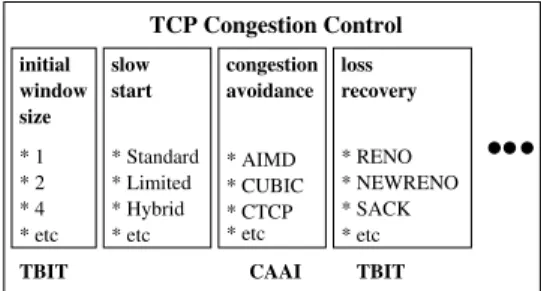
II. TCP CONGESTIONCONTROL ANDRELATEDWORKS TCP congestion control consists of several important com-ponents, such as the initial window size, slow start, congestion avoidance, loss recovery, etc, as illustrated in Figure 1. The initial window size could be 1, 2 [25], 3, 4 [26], or even 10 [27] packets. The slow start algorithm could be the standard slow start [25], limited slow start [28], hybrid slow start [29], etc. The congestion avoidance algorithm could be AIMD [1], CU-BIC [13], CTCP [7], etc. The loss recovery mechanism could be RENO [30], NEWRENO [31], SACK [32], DSACK [33], etc. Note that, we can create different TCP congestion control algorithms with different combinations of these components. For example, CUBIC can be combined with the standard slow start or the hybrid slow start or other slow start algorithms,

TBIT * 2 * 4 * etc * Standard * Limited * Hybrid * etc * AIMD * CUBIC * CTCP * etc * RENO * NEWRENO * SACK * etc initial size window slow start congestion avoidance loss recovery TCP Congestion Control CAAI TBIT * 1

Fig. 1. TCP congestion control components.

and it can be combined with NEWRENO or SACK or other loss recovery mechanisms.

CAAI proposed in this paper only considers how to identify the TCP congestion avoidance component of a web server. The initial window size and the loss recovery components of a web server can be identified by TBIT [34] (described later in this section). Very few slow start algorithms have been implemented in major operating systems, and therefore, we do not consider how to identify them in this paper.

Because this paper only considers the congestion avoidance component of a TCP congestion control algorithm, we use

a TCP congestion avoidance algorithm or a TCP algorithm

to refer to the congestion avoidance component of a TCP congestion control algorithm. For example, when we say that a TCP algorithm is CUBIC, it means that the conges-tion avoidance component of the TCP congesconges-tion control algorithm is CUBIC. Below, we first review related works on identifying TCP congestion avoidance components, and then review related works on inferring other TCP congestion control components.

1) Related works on identifying TCP congestion avoidance

components: Because most TCP algorithms listed in Table I

were proposed recently, there are very few papers on iden-tifying them. Oshio et al. [35] propose a cluster analysis-based method for a router to distinguish between two different TCP algorithms. Feyzabadi et al.[36] consider how to detect whether the TCP algorithm of a web server is AIMD or CUBIC. Our proposed CAAI is different from their works in that 1) CAAI can distinguish among most TCP algorithms available in major operating system families, whereas their works consider only two different TCP algorithms; 2) we have solved many web and TCP issues so that we can conduct a large scale of Internet experiments, whereas their works are mainly based on simulations.

Our early work [37] proposes a method to infer the TCP multiplicative decrease parameter of a web server, which is an important TCP feature for identifying TCP algorithms. This paper differs from our early work [37] in the following ways. 1) This paper considers how to distinguish among different TCP algorithms; whereas our early work only considers how to extract a TCP feature - the TCP multiplicative decrease parameter; and 2) this paper presents, for the first time, the TCP deployment information of the 5000 most popular web servers.

(4)

2) Related works on inferring other TCP congestion control components: There are a large number of papers on inferring other TCP congestion control components, and they can be classified into two categories: active measurements [38], [34], [39], [40] which actively measure the TCP behaviors of Internet nodes, and passive measurements [41], [42], [43], [44], [45] which measure the TCP behaviors of Internet flows in passively collected packet traces. Below, we review the two most relevant works.

TBIT [34] is a popular active measurement tool for inferring TCP behavior of a remote web server. It can infer various TCP behaviors such as the initial window size, the loss recovery mechanisms, congestion window halving, etc. But it cannot identify the congestion avoidance algorithms, simply because most congestion avoidance algorithms listed in Table I were proposed after TBIT was developed. CAAI is implemented by extending the source code of TBIT. Specifically, CAAI only uses part of the TBIT code to communicate raw TCP packets with a web server. We wrote our own code to emulate two network environments, to extract two TCP features, and to identify the TCP congestion avoidance algorithm.

NMAP [40] is a popular active measurement tool for inferring the information, such as the operating system, of a remote Internet node. However, it is hard to infer the TCP algorithm of a remote Internet node, even if we can detect the operating system of the node for the following reasons. Even though an operating system has a default TCP algorithm, a user can easily change the default algorithm. For example, both Windows and Linux users can change the default algorithm with only a single line of command. Furthermore, different versions of the same operating system may have different default algorithms. For example, different Linux kernels may have different default TCP algorithms, and moreover different Linux distributions may have different default TCP algorithms.

III. CAAI OVERVIEW

A. Design Goals

CAAI is designed to actively identify the TCP congestion avoidance algorithm of a remote web server. We have the following design goals for CAAI.

• Design goal 1: It can identify all default TCP algorithms

and most non-default TCP algorithms of major operating system families.

• Design goal 2: It is insensitive to the operating system

of a web server, insensitive to network conditions, and insensitive to TCP components other than the congestion avoidance component.

For the first design goal, we consider a total of 13 TCP algorithms: AIMD [1], BIC [12], CTCP [7], CUBIC’ and CUBIC [13], HSTCP [14], HTCP [15], ILLINOIS [17], STCP [19], VEGAS [20], VENO [21], WESTWOOD+ [22], and YEAH [23]. AIMD is the default TCP of some Windows operating systems, and some Linux operating systems. CTCP is the default TCP of some Windows operating systems. BIC and CUBIC are the default TCP of some Linux operating

systems. Since CUBIC was included into Linux Kernel in 2006, it has had several major changes [13]. We consider two major versions of CUBIC: Linux kernel 2.6.25 and before referred to as CUBIC’, and Linux kernel 2.6.26 and after referred to as CUBIC. Finally, among all TCP algorithms listed in Table I, we do not consider two TCP algorithms: HYBLA [16] and LP [18], because they are not designed for web servers. Specifically, HYBLA [16] is primarily designed for satellite connections, and LP [18] is designed for back-ground file transfer.

The second design goal enables us to accurately identify the TCP algorithms of as many web servers as possible. Insensitiv-ity to the operating system of a web server is desirable because the same TCP algorithm can be implemented into different operating systems. Insensitivity to network conditions (e.g., packet loss, delay, reordering, and duplication) is desirable because we have no control of the network condition between a CAAI computer and a remote web server. Insensitivity to TCP components other than congestion avoidance is desirable, because the TCP behavior of a web server is controlled not only by its TCP congestion avoidance component but also by many other TCP components (as listed in Figure 1).

B. TCP Algorithm Features

A TCP congestion avoidance algorithm can be well de-scribed by the following two features.

• Feature 1: Multiplicative Decrease Parameter (denoted

byβ), which determines the slow start threshold (i.e., the boundary congestion window size between the slow start and congestion avoidance states).

• Feature 2: Window Growth Function (denoted by g(·)),

which determines how a TCP algorithm grows its con-gestion window size in the concon-gestion avoidance state. Let loss cwnd denote the congestion window size just before a loss event or a timeout. In case of a loss event, TCP sets both its slow start threshold and congestion window size to β×loss cwnd. In case of a time out, TCP sets its slow start threshold toβ×loss cwnd, and sets its congestion window size to usually 1 packet. Different TCP algorithms usually have different multiplicative decrease parameters. For example, AIMD sets β = 0.5; CUBIC sets β = 0.7; and STCP setsβ = 0.875. Some TCP algorithms have a variable β which depends onloss cwndand the network environment such as the duration of a round-trip time (RTT), the minimum RTT, and the maximum RTT. For example, BIC setsβ = 0.8

if loss cwnd > 14, and sets β = 0.5 if loss cwnd ≤ 14; HSTCP setsβ between 0.5 and 0.9 depending onloss cwnd; HTCP sets β between 0.5 and 0.8 depending on the ratio of the minimum RTT and the maximum RTT.

Different TCP algorithms usually have different window growth functions. The window growth function of a TCP algorithm is usually a function of the elapsed number of RTTs in the congestion avoidance state (denoted by x) and loss cwnd. For example, AIMD has a linear window growth function ofx(i.e.,g(x, loss cwnd) = 0.5×loss cwnd+x); and STCP has an exponential window growth function of x

(5)

(i.e.,g(x, loss cwnd) = 0.875×loss cwnd×1.02x

for non-delayed ACKs). Some TCP algorithms have a window growth function which depends not only onx, but also on the network environment. For example, the CUBIC function depends on both x and the duration of an RTT; and the CTCP function depends onx, the duration of an RTT, and the minimum RTT. Note that different TCP algorithms may show different features in a network environment, but show the same features in another network environment. Therefore, an important part of CAAI is to emulate some network environments in which different TCP algorithms have different features so that they can be distinguished from one another.

C. CAAI Steps

CAAI identifies the TCP algorithm of a remote web server by analyzing the TCP behaviors of the web server in some emulated network environments. CAAI has the following three steps.

• Step 1: Trace Gathering. CAAI gathers the TCP

con-gestion window traces of a remote web server in some emulated network environments.

• Step 2: Feature Extraction. CAAI extracts the two TCP

algorithm features from the gathered TCP congestion window traces.

• Step 3: Algorithm Classification. CAAI finally identifies

the TCP algorithm by comparing the extracted features with the training features.

D. Design Challenges

It is very challenging to design CAAI for the following reasons. 1) It might be easy to find a network environment to distinguish 2 TCP algorithms, however, it is nontrivial to find a small set of network environments to clearly distinguish a large number of TCP algorithms, like 13 TCP algorithms. 2) We do not have the control of the network condition between a CAAI computer and a remote web server. The condition of the network from a remote web server to a CAAI computer greatly influences the TCP data packets sent from the web server. The condition of the network from a CAAI computer to a web server greatly influences the TCP ACK packets received by the web server. Therefore, it is hard to emulate desired network environments, hard to measure the TCP congestion window sizes of a web server, hard to extract TCP features from the measured congestion window traces, and hard to identify the TCP algorithm based on the extracted TCP features. 3) We do not have control of the content on a web server, and most web pages are very short. Therefore, it is hard to maintain a TCP connection between a CAAI computer and a remote web server long enough so that CAAI can gather sufficiently long traces of TCP congestion window sizes.

IV. CAAI STEP1: TRACEGATHERING

A. Overview

The first step of CAAI gathers the traces of TCP congestion window sizes of a remote web server in some emulated

network environments. These network environments are care-fully chosen so that different TCP algorithms have different features and thus they can be distinguished from one another. Specifically, for each network environment,

• Subtask 1:CAAI creates a TCP connection to a remote

web server and emulates the network environment.

• Subtask 2: CAAI measures the TCP congestion window

sizes of the web server in the emulated network environ-ment.

• Subtask 3: CAAI maintains the TCP connection until

it has gathered a sufficiently long trace of congestion window sizes.

B. Emulated Network Environments

CAAI emulates the following two network environments with parameters timeout and mss for a web server.

Net-work Environment A: CAAI sends back an ACK packet to

acknowledge each TCP data packet from the web server (i.e., non-delayed ACKs). The TCP data packets sent from the web server are not lost until the TCP congestion window size of the web server becomes greater than timeout packets. Then, the packet loss leads to a TCP timeout of the web server (i.e., loss cwnd≥timeout). After the timeout, there is again no data packet loss. In addition, there is always no data packet reordering in the emulated network. The maximum TCP segment size (MSS) ismssbytes, and the RTT between CAAI and the web server is always 1.0 second. Network Environment B:Same as network environment A, except that the RTT is 0.8 or 1.0 seconds as specified in Figure 2.

0 0.2 0.4 0.6 0.8 1 1.2 0 10 20 30 40 50 60 Emulated RTT (Seconds)

No. of Emulated RTTs before Timeout Network Environment A Network Environment B

(a) Before Timeout

0 0.2 0.4 0.6 0.8 1 1.2 0 5 10 15 20 25 Emulated RTT (Seconds)

No. of Emulated RTTs after Timeout Network Environment A Network Environment B

(b) After Timeout Fig. 2. The RTTs of the two emulated network environments A and B.

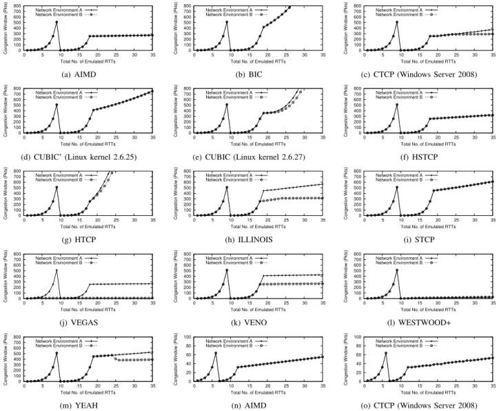
Why these two network environments?Figure 3 shows the

traces of congestion window sizes of all 13 TCP algorithms in these two network environments. We can see that network environment A or B alone is insufficient to distinguish among 13 TCP algorithms. For example, AIMD (Figure 3(a)) and VEGAS (Figure 3(j)) have the same trace in network envi-ronment A, and AIMD (Figure 3(a)) and VENO (Figure 3(k)) have very similar traces in network environment B. Both A and B together withtimeout= 512packets can clearly distinguish among all 13 TCP algorithms. Network environment A is used to collect the behavior of a TCP algorithm in a network environment with a fixed RTT, in which we can extract two TCP features for a fixed RTT. Network environment B is used to collect the behavior of the TCP algorithm in another network environment with a varying RTT, in which we can extract another two TCP features for a varying RTT. Before the timeout in network environment B, RTT increases from

(6)

0 100 200 300 400 500 600 700 800 0 5 10 15 20 25 30 35 Congestion Window (Pkts)

Total No. of Emulated RTTs Network Environment A Network Environment B (a) AIMD 0 100 200 300 400 500 600 700 800 0 5 10 15 20 25 30 35 Congestion Window (Pkts)

Total No. of Emulated RTTs Network Environment A Network Environment B (b) BIC 0 100 200 300 400 500 600 700 800 0 5 10 15 20 25 30 35 Congestion Window (Pkts)

Total No. of Emulated RTTs Network Environment A Network Environment B (c) CTCP (Windows Server 2008) 0 100 200 300 400 500 600 700 800 0 5 10 15 20 25 30 35 Congestion Window (Pkts)

Total No. of Emulated RTTs Network Environment A Network Environment B

(d) CUBIC’ (Linux kernel 2.6.25)

(e) CUBIC (Linux kernel 2.6.27)

Total No. of Emulated RTTs Network Environment A Network Environment B (f) HSTCP 0 100 200 300 400 500 600 700 800 0 5 10 15 20 25 30 35 Congestion Window (Pkts)

Total No. of Emulated RTTs Network Environment A Network Environment B (g) HTCP 0 100 200 300 400 500 600 700 800 0 5 10 15 20 25 30 35 Congestion Window (Pkts)

Total No. of Emulated RTTs Network Environment A Network Environment B (h) ILLINOIS 0 100 200 300 400 500 600 700 800 0 5 10 15 20 25 30 35 Congestion Window (Pkts)

Total No. of Emulated RTTs Network Environment A Network Environment B (i) STCP 0 100 200 300 400 500 600 700 800 0 5 10 15 20 25 30 35 Congestion Window (Pkts)

Total No. of Emulated RTTs Network Environment A Network Environment B (j) VEGAS 0 100 200 300 400 500 600 700 800 0 5 10 15 20 25 30 35 Congestion Window (Pkts)

Total No. of Emulated RTTs Network Environment A Network Environment B (k) VENO 0 100 200 300 400 500 600 700 800 0 5 10 15 20 25 30 35 Congestion Window (Pkts)

Total No. of Emulated RTTs Network Environment A Network Environment B (l) WESTWOOD+ 0 100 200 300 400 500 600 700 800 0 5 10 15 20 25 30 35 Congestion Window (Pkts)

Total No. of Emulated RTTs Network Environment A Network Environment B (m) YEAH 0 20 40 60 80 100 0 5 10 15 20 25 30 35 Congestion Window (Pkts)

Total No. of Emulated RTTs Network Environment A Network Environment B (n) AIMD 0 20 40 60 80 100 0 5 10 15 20 25 30 35 Congestion Window (Pkts)

(o) CTCP (Windows Server 2008)

Fig. 3. The traces of congestion window sizes of all 13 TCP algorithms in network environments A and B measured on our local testbed with a 0% packet loss rate. The first 13 figures ((a) to (m)) are obtained withtimeout= 512_{packets, and the last 2 figures ((n) and (o)) are obtained with}timeout= 64_packets.

The results remain the same for all different values ofmss_{. Unless explicitly indicated, the operating system is Linux kernel 2.6.27. We can see that two} network environments A and B withtimeout= 512_{packets can be used to clearly distinguish among all 13 TCP algorithms. However, with}timeout= 64

packets, AIMD and CTCP have the same traces. Not shown in the figure, the other 11 TCP algorithms still have different traces withtimeout= 64_packets.

0.8 to 1.0 second after the 3rd RTT, and this is used to check whether theβfeature depends on RTT (e.g., ILLINOIS shown in Figure 3(h) and VENO shown in Figure 3(k)). After the timeout, RTT increases from 0.8 to 1.0 second after the 12th RTT, and this is used to check whether theg(·)feature depends on RTT (e.g., CTCP shown in Figure 3(c) and YEAH shown in Figure 3(m)). As explained below, timeout is always no more than 512 packets, and therefore, TCP has already entered the congestion avoidance state after 12 RTTs.

Values of timeout: Most TCP algorithms typically have

the same or similar behavior as the traditional AIMD for small congestion window sizes (e.g., CTCP=AIMD when their congestion window sizes are less than 41), and have different behaviors than AIMD for large congestion window sizes. Therefore, congestion window traces obtained with a large timeout can be used to accurately distinguish among different TCP algorithms. For example, Figure 3 shows that

two network environments A and B with timeout = 512

packets can be used to clearly distinguish among all 13 TCP algorithms. But, with timeout = 64 packets, AIMD and CTCP have the same traces of congestion window sizes, and the other 11 TCP algorithms still have different traces (not shown in the paper). However, congestion window traces with a very largetimeoutare hard to obtain, because they require a very long web page to be downloaded from the web server which is usually time-consuming and sometimes impossible to find on the web server, and because the maximum achievable congestion window size is affected by many factors such as the bandwidth-delay product of the network and the service load of the web server. CAAI tries four timeout values in the decreasing order of 512, 256, 128, and 64 packets. This is because traces withtimeout greater than 512 are sometimes hard to obtain, and traces withtimeoutless than 64 is almost useless for distinguishing among different TCP algorithms.

(7)

Values ofmss:Since the maximum congestion window size is limited by the ratio of the bandwidth-delay product to the MSS, we should set mssto a smaller value in order to have a higher maximum congestion window size. CAAI tries four mssvalues in the increasing order of 100, 300, 536, and 1460 bytes. This is because previous Internet measurement [39] shows that a large fraction of web servers accept an MSS as low as 100 bytes, and all web servers accept an MSS of 1460 bytes.

Why emulating an RTT of 1.0 second?Because we can only emulate an RTT longer than the actual RTT between a CAAI computer and a web server, and because we want to emulate the same two network environments for all web servers, the emulated RTT should be longer than all actual RTTs. However, a very long emulated RTT may cause undesired TCP timeouts (actual TCP timeouts, not our emulated TCP timeout). Figure 4 shows the cumulative distribution function (CDF) of the actual RTTs of the 5000 most popular web servers that we measured in November 2010, and we can see that almost all actual RTTs are less than 0.8 seconds. In addition, the initial TCP timeout period is usually between 2.5 and 6.0 seconds [46], but some web servers may have shorter initial TCP timeout periods. Therefore, we can choose an emulated RTT in the range of 0.8 seconds and 2.5 seconds, and CAAI chooses 1.0 second.

0 0.2 0.4 0.6 0.8 1 0 0.2 0.4 0.6 0.8 1 CDF

Round Trip Time (Seconds)

Fig. 4. The cumulative distribution function (CDF) of the RTT of the 5000 most popular web servers. Measured in November 2010. One RTT per web server.

Why emulating a timeout (i.e., no ACK packet until the time-out) instead of a loss event (i.e., three duplicate ACK packets)?

This is because right after a loss event, the congestion window size depends not only on the congestion avoidance algorithm, but also heavily on some other TCP components such as burstiness control in Linux. Linux uses a special burstiness control [47], [48] to prevent TCP from sending a burst of packets to the Internet, since bursty traffic may cause long queueing delay and high packet loss. However, the burstiness control interferes with congestion control on controlling the TCP congestion window size. For example, for a Linux web server, the congestion window size right after a loss event may be far less than β×loss cwnd, and therefore, it is hard to accurately measure the two TCP features after a loss event.

Why not combining multiple network environments into one

longer network environment? A longer network environment

requires a longer web page to be downloaded from a web server, which is usually time-consuming and sometimes im-possible to find. Therefore, we prefer multiple short network environments rather than a long network environment.

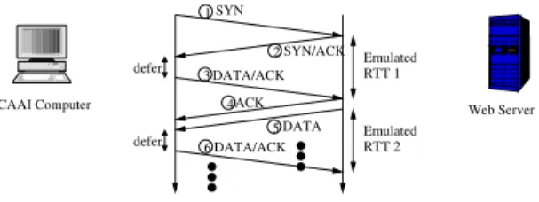
1 6 3 2 5 4 Emulated RTT 1 Emulated RTT 2 defer defer SYN DATA/ACK DATA/ACK SYN/ACK DATA ACK Web Server CAAI Computer

Fig. 5. TCP packets between CAAI and a remote web server.

C. Subtask 1: Emulating a Network Environment

Figure 5 illustrates how CAAI communicates with a web server and how it emulates a network environment. CAAI first establishes a TCP connection to the web server by sending a SYN packet (number 1 in the figure). The SYN packet contains a TCP option to set MSS to mss and another TCP option to enable the window scaling. After receiving the SYN/ACK packet (number 2) from the web server, CAAI defers sending the first DATA/ACK packet (number 3) for a while so that the first RTT experienced by the web server is as long as the first RTT of the emulated network environment. This DATA/ACK packet not only acknowledges the SYN/ACK packet, but also contains the first few HTTP request messages.

The web server sends back an ACK packet (number 4) to acknowledge the DATA/ACK packet, and then sends its data packets (only the first packet, number 5, is shown in the figure) which contain HTTP response messages. CAAI again defers sending the next DATA/ACK packet (number 6) so that the second RTT experienced by the web server is as long as the second RTT of the emulated network environment. This DATA/ACK packet not only acknowledges the received data packet (number 5), but also contains the next few HTTP request messages. CAAI continues acknowledging each received data packet, until the TCP congestion window size of the web server is greater thantimeout. Then, CAAI stops sending any packet, and therefore the TCP algorithm of the web server will finally timeout and retransmit the lost packets. For each data packet received after the timeout, CAAI sends back a DATA/ACK which acknowledges all data packets received so far. CAAI finally stops after the web server does not send any more data packets or after it has gathered a sufficient long trace.

How to emulate a network without any loss or reordering of data packets except the timeout? Since CAAI defers sending ACK packets, it can detect most lost and reordered packets by checking the sequence numbers of data packets received from the web server. In case of packet loss or reordering, CAAI still sends the correct ACK packets as if there is no packet loss or reordering. Note that, however, CAAI cannot guarantee that ACK packets will be successfully delivered to the web server, and this is a major reason for the inaccuracy of CAAI identification results.

How to deal with forward RTO-recovery (F-RTO)[49]?The

emulated TCP timeout may be detected by a web server using F-RTO as a spurious retransmission timeout. In this case, the web server does not have a regular slow start after the emulated timeout, which is however required by CAAI to accurately

(8)

determine the two TCP features. Therefore, for web servers using F-RTO, CAAI sends a duplicate ACK after the emulated timeout in order to stop the F-RTO recovery and start the conventional TCP timeout recovery.

How to deal with slow start threshold caching? Usually, the initial slow start threshold of a new TCP connection is set to infinite. However, a web server using slow start threshold caching (as part of TCP auto-tuning) sets the initial slow start threshold of a new TCP connection to the slow start threshold of the previous TCP connection of the same web client. In this case, if CAAI emulates network environment B immediately after network environment A, the web server exits the slow start state very early and takes a very long time to reach timeout. Therefore, for web servers using slow start threshold caching, CAAI waits for some time (like 10 minutes) between emulating network environments A and B.

D. Subtask 2: Measuring the Congestion Window Sizes

We estimate the TCP congestion window size of a web server by the number of data packets that it sends in an emulated RTT. There are two difficulties. 1) After CAAI receives a data packet from the web server, how to determine whether it belongs to the previous RTT or the current RTT? 2) Since a packet may be lost or duplicated in the Internet, the number of data packets received by CAAI may not be equal to the number of data packets sent by the web server.

The first difficulty can be solved by emulating an RTT long enough so that the bandwidth-delay product is much larger thantimeout×mss. In this way, the web server sends all data packets belonging to the same emulated RTT in a short time interval at the beginning of an emulated RTT. After receiving all corresponding ACK packets in a short time interval at the beginning of the next emulated RTT, the web server sends all data packets belonging to the next emulated RTT in a short time interval at the beginning of the next emulated RTT. Therefore, there is a long time gap between two consecutive data packets belonging to two different emulated RTTs. Considering that the maximum timeout of CAAI is 512 packets and the maximum mss of CAAI is 1460 bytes, if the bandwidth from a web server to a CAAI computer is at least 10 Mbps, an emulated RTT should be longer than

512×1460×8/107

= 0.6 seconds. The emulated RTTs of both network environments are 1.0 and 0.8 seconds which are longer than 0.6 seconds.

The second difficulty can be solved by using the highest sequence number among all data packets which CAAI receives in an emulated RTT. CAAI measures the congestion window size wk of the web server at RTT kas follows:wk = (hk−

hk₋1)/msswhere hk is the highest sequence number among

all data packets which CAAI receives in the kth RTT. In this way, as long as CAAI receives the data packet with the highest sequence number, it can accurately measure the congestion window size. Even if the data packet with the highest sequence number is lost, CAAI can still reasonably accurately measure the congestion window size as long as it receives the data packets with the next highest sequence numbers.

E. Subtask 3: Maintaining a TCP connection

In order to distinguish among different TCP algorithms, CAAI must gather sufficiently long traces of congestion win-dow sizes. Because timeout is no more than 512 packets, the slow start state usually takes no more than 10 RTTs. Therefore, CAAI gathers at least 16 RTTs of congestion window sizes after the timeout so that TCP has usually entered the congestion avoidance state for at least 6 RTTs, which is the minimum number of RTTs (as shown in Figure 3) to dis-tinguish among all 13 TCP algorithms whentimeout= 512

packets. Accordingly, we define a valid trace to be a trace which has at least 16 RTTs of congestion window sizes after the timeout. CAAI gathers at most 25 RTTs of congestion window size after the timeout, at which time TCP has usually entered the congestion avoidance state for at least 15 RTTs which is sufficiently long for distinguish among all 13 TCP algorithms. Overall, CAAI continues gathering a trace, until there is no data packet from the web server or until 25 RTTs after the timeout.

The difficulty is how to maintain the TCP connection so that CAAI can gather a valid trace of congestion window sizes. For example, for network environment A and B withtimeout= 512 packets and mss = 100 bytes, it requires about 340K bytes of data for a web server with AIMD to send a total of 26 RTTs of data packets (10 RTTs before timeout and 16 RTTs after timeout). Formss= 300, 536, and 1460 bytes, it requires about 1000K, 1800K, and 4900K bytes, respectively. CAAI uses the following two methods together to solve the problem.

First, CAAI repeatedly sends the same HTTP request mes-sage to a web server. One might think that it is sufficient to repeatedly request the default index.html of a web server. However, there are two issues. 1) A considerable fraction of web servers only accept the first or the first few HTTP requests, and discard the remaining requests. 2) Some web servers have a very short index.html.

Second, CAAI sends HTTP request messages for a long web page. We have developed a web page searching tool to automatically search a web server for a long web page (e.g., html files, image files, or executable files). Specifically, for a web server, our tool first uses httrack [50] to find as many webpages as possible in 5 minutes (while taking care of http redirection), uses the dig service to find web pages belonging to the same domain as the web server, obtains the web page headers to find their sizes without actually downloading them, and finally finds the longest web pages. It turns out that this is the most time-consuming part of our experiments, and therefore we run this tool simultaneously on hundreds of Planetlab nodes [51].

V. CAAI STEP2: FEATUREEXTRACTION

This section describes how CAAI extracts the two features from a trace of n congestion window sizes: w1, w2, ..., wo, wo+1, ..., wn, where wo is the congestion

win-dow size right before the timeout, and wo+1 is the first

(9)

valid trace, we haveo+16≤n≤o+25. In order to extract the two features, CAAI first determines at which RTT (denoted by s, and called the threshold RTT) after the timeout TCP leaves the slow start state. That is, the slow start threshold is between ws₋1 andws. Once the threshold RTT is determined, the two

features can be easily extracted.

A. Determining the Threshold RTT

The determination of the threshold RTT is based on the fact that the standard TCP slow start is usually the default one, and the hybrid slow start [29] used by CUBIC behaves the same as the standard slow start in our emulated network environments A and B (since the RTTs of the slow start state after the timeout remain unchanged, and the emulated RTT is relatively long). That is, a TCP algorithm increases the congestion window size by one for every received ACK in the slow start state and increases the congestion window size relatively slowly in the congestion avoidance state. The challenge is how to check whether the congestion window size of a web server is increased by one for every ACK packet when ACK packets may be lost. To solve this problem, CAAI first estimates the maximum ACK loss rate in the slow start state, and then uses it to determine the threshold RTT.

At an RTT in the slow start state after the timeout, say RTT k > o+ 1, CAAI estimates the maximum ACK loss rate (denoted by pk) on the path from CAAI to a web server by

the following equation, which is obtained using the interval estimation technique with a confidence level of 99.9%.

pk= 2n2+ 3.272+ 3.27 p 4n2(n1−n2)/n1+ 3.272 2(n1+ 3.272) (1) where n1=P k₋1

i=o+1wi is the total number of ACK packets

sent since the timeout, and n2 = P k₋1

i=o+1(2wi −wi+1) is

the total number of lost ACK packets since the timeout. The number 2wi −wi+1 is an estimate of the number of ACK

packets lost in RTT i. This is because CAAI sends wi ACK

packets at RTTi, and if all of them are successfully received by the web server, the congestion window size wi+1 at RTT

i+ 1 should be2wi. To avoid abnormal pk values, we limit

the maximum pk to be 80%, and the minimumpk to be 5%.

CAAI detects whether the congestion window size at RTT k is increased by one for every ACK packet by checking whetherwk+1> wk+wk(1−pk). Starting from the smallest

RTT s > o such that ws ≥ wo/2, CAAI searches for four

consecutive RTTss−1,s,s+1, ands+2, for all of which the congestion window size is not increased by one for every ACK packet. RTT s is then the threshold RTT. This method can more accurately determine the threshold RTT than the method proposed in our early work [37] as evaluated in Section VII.

B. Feature 1: Multiplicative Decrease Parameter

Feature β can be obtained by β = ws/loss cwnd where

ws is the congestion window size at the threshold RTT, and

loss cwnd is the congestion window size right before the timeout (i.e., loss cwnd=wo). If the extracted β is greater

than 1.0, CAAI reports an abnormal slow start error.

C. Feature 2: Window Growth Function

The window growth function of a trace can be described by the congestion window sizes after RTTs. We use a fifth-degree polynomialg(x) =a0+a1x+a2x2+a3x3+a4x4+a5x5 to

fit the congestion window sizes after RTTs. There are three reasons. 1) Different traces may have different RTT numbers of congestion window sizes, with curve fitting CAAI can use six coefficients to describe a trace with any RTT number of congestion window sizes. 2) For the 13 TCP algorithms, most of their window growth functions can be well fitted with a first-degree polynomial (i.e., a linear function for AIMD), some of them can be well fitted with a third-degree polynomial (i.e., a cubic function for CUBIC), and the window growth function of YEAH in network environment B can be well fitted with a fifth-degree polynomial. Note that although the actual window growth function of STCP is an exponential function, its traces within the first tens of RTTs after RTTscan be well fitted with a first-degree polynomial. 3) A trace of congestion window sizes may have some noises due to some network and server factors, and curve fitting can greatly eliminate these noises.

In addition, we fit the offset congestion window sizes (i.e., g(1) =ws+1−ws,g(2) =ws+2−ws, ...) instead of the actual

congestion window sizes (i.e.,g(1) =ws,g(2) =ws+1, ...).

The advantage is that for most TCP algorithms, we can use the sameg(x)and thus the same set of coefficients to describe the window growth function of traces with differencews values.

For example,g(x)is always xfor AIMD traces.

D. The Feature Vectors of a Web Server

CAAI emulates two network environments A and B, and gathers two traces from a web server. All the features of a web server can be described by a feature vectorV = (βA

,aA 0,a A 1, aA 2,a A 3,a A 4,a A 5,β B ,aB 0,a B 1,a B 2,a B 3,a B 4,a B 5). Features with

superscripts A andB are for network environments A and B, respectively. Sometimes, a TCP algorithm does not experience any timeout for a network environment (e.g., VEGAS in network environment B as shown in Figure 3(j)). In this case, CAAI setsβ to -1, and fitsg(x)to the whole trace.

VI. CAAI STEP3: ALGORITHMCLASSIFICATION This section describes how CAAI identifies the TCP al-gorithm of a web server based on its feature vector V. The challenge is that we may get different feature vectors for different web servers with the same TCP algorithm or for the same web sever but at different times. This is because the congestion window trace gathered from a web server depends on the network condition, especially the instantaneous ACK loss rate on the path from a CAAI computer to the web server. To solve this problem, we create a training set which contains the feature vectors of all TCP algorithms in some network conditions (details in Section VII). Among all feature vectors in the training set, CAAI finds the one which is the closest to the feature vector of a web server.

We now describe some necessary notation. We refer to the feature vector of a web server as theweb feature vector, and denote it byV = (βA ,aA 0,a A 1,a A 2,a A 3,a A 4,a A 5,β B ,aB 0,a B 1,

(10)

aB 2, a B 3, a B 4, a B

5). Its window growth functions in network

environments A and B aregA

(x)andgB (x), respectively. For example,gA (x) =aA 0 +a A 1x+a A 2x 2 +aA 3x 3 +aA 4x 4 +aA 5x 5 . We refer to a feature vector in the training set as a training feature vector, and denote it by V´ = ( ´βA

,aÁ 0, á A 1,á A 2, á A 3, ´ aA 4, á A 5, β´ B , áB 0, a´ B 1, a´ B 2, á B 3, á B 4, á B

5). Its window growth

functions in network environments A and B are g´A₍_x₎

and

´

gB₍_x₎

, respectively.

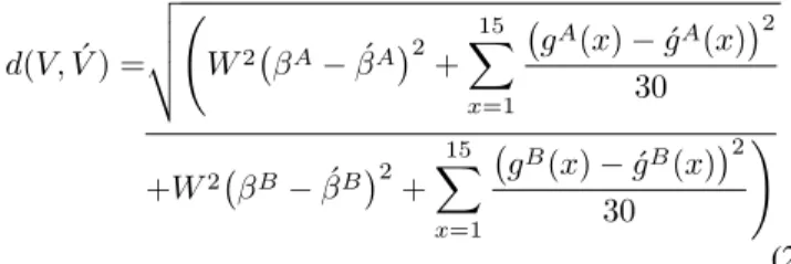
For a web feature vector V, CAAI finds the closest one among all training feature vectors with the same timeout value as the web feature vector. The distance between two feature vectorsV andV´ is defined as follows.

d(V,V´) = v u u t W2 βA−β´A 2 + 15 X x=1 gA₍_x₎₋_g_´A₍_x₎2 30 +W2 _βB₋_β´B2 + 15 X x=1 gB₍_x₎₋_´_gB₍_x₎2 30 ! (2) where the first and third terms inside the square root are the weighted difference between twoβfeatures (W is the weight), and the second and fourth terms are the normalized differences between the corresponding points of the two window growth functions. The number 15 is because CAAI usually gathers 25 RTTs of congestion window size after a timeout (described in Section IV-E), and thus TCP has entered the congestion avoidance state for at least 15 RTTs (when timeout≤512).

If the distance between the web feature vector and the closest training feature vector is less than a threshold D, CAAI reports the TCP algorithm of the closest training feature vector as the identification result. Otherwise, CAAI reports that the web server uses an unknown TCP algorithm, since the web feature vector is too far away from every training feature vector. Overall, CAAI has a total of two parameters. Parameter W is the weight ofβ features, and parameterD is the maximum allowed distance.

VII. CAAI EXPERIMENTS

In this section, we describe our CAAI experiment results. The CAAI experiments described in this paper are not de-signed to comprehensively measure the deployment informa-tion of different TCP algorithms on web servers, and they are only used to demonstrate the potential applications of CAAI.

A. Collecting Training Feature Vectors

We use our lab test-bed to collect training feature vectors for CAAI. The test-bed consists of four computers: one CAAI computer, one Linux web server, one Windows web server, all connected to a Linux router. The Linux web server runs Apache, and the Windows web server runs IIS. We run Netem [52] on the Linux router to emulate various network conditions between the CAAI computer and a web server. Specifically, we emulate 2 network conditions with different RTTs: 50ms and 250 ms, corresponding to two types of web servers: web servers close to or far away from the CAAI

computer. In both network conditions, there is no packet loss for both TCP data and ACK packets.

The feature vectors of CTCP are obtained using an IIS web server on Windows Server 2008, the feature vectors of CUBIC’ are obtained using an Apache server on Linux kernel 2.6.25, and the feature vectors of all other 11 TCP algorithms are obtained using an Apache server on openSUSE 11.1 with Linux kernel 2.6.27. Note that, we use the feature vectors of AIMD only in Linux. This is because there is only slightly difference between AIMD in Linux and AIMD in Windows, and the slight difference would not noticeably affect the identification accuracy for AIMD.

For each of 2 network conditions between the CAAI com-puter and a web server, for each of 4timeoutvalues (i.e., 512, 256, 128, and 64 packets), and for each of 13 TCP algorithms, we collect a training feature vector which contains the features of a TCP algorithm in network environments A and B with timeout. Note that the value of mss has no impact on the feature vectors. Therefore, there are a total of2×4×13 = 104

training feature vectors. However, note that when classifying a web feature vector, CAAI compares it only with the training feature vectors with the sametimeoutvalue as the web feature vector. For example, when classifying a web feature vector withtimeout= 512packets, CAAI only uses the2×13 = 26

training feature vectors withtimeout= 512 packets.

We notice that AIMD and CTCP behave very similar to each other whentimeout is 128 or 64 packets, and consequently, AIMD and CTCP have very similar feature vectors in these cases. Therefore, whentimeout is 128 or 64 packets, we do not distinguish between AIMD and CTCP.

B. Testbed Evaluation and Validation

1) Parameter Setting and Validation: In order to set the parameters of CAAI and evaluate the identification accuracy of CAAI, we collect a set of validation feature vectors obtained using 10 packet loss rates (the 0% training packet loss rate plus 9 new packet loss rates: 0.01%, 0.02%, 0.05%, 0.1%, 0.2%, 0.5%, 1%, 2%, and 5%), 5 RTTs (the 2 training RTTs plus 3 new RTTs: 100, 150, and 200 ms), the same 4timeoutvalues, and the same 13 TCP algorithms. Therefore, there are a total of 10×5×4×13 = 2600validation feature vectors.

We use CAAI with the 104 training feature vectors to identify all 2600 validation feature vectors. In order to choose the value of parameter W, we temporarily set D to infinite so that no unknown TCP algorithm is reported (i.e., each validation feature vector is identified as some TCP algorithm). Figure 6 shows the identification accuracy of CAAI when parameterW varies from 1 to 16384. The identification accu-racy is the percentage of correctly identified validation feature vectors. After checking the incorrectly identified validation feature vectors, we found that in network conditions with high packet loss rates, CAAI sometimes cannot correctly distinguish between AIMD and VENO which have similar window growth functions, and sometimes cannot correctly distinguish between ILLINOIS and STCP which have similar window growth functions.

(11)

We can see that CAAI achieves the best accuracy when W is around 256, and a very small or very big W impairs the identification accuracy. Intuitively, this is because in one extreme case when W is very small, CAAI mainly uses the window growth function feature (i.e., g(·)), and in another extreme case when W is very big, CAAI mainly uses the multiplicative decrease parameter feature (i.e.,β). Only when W is neither small nor big, CAAI uses both features and thus can achieve better identification accuracy. Therefore, CAAI setsW to 256, at which point CAAI achieves an identification accuracy of 95.7%. Finally, with W = 256, we set parameter D to the maximum distance between a validation feature vector and its closest training feature vector, which is about 500.

2) Evaluating the Threshold RTT: We evaluate our method which detects the threshold RTT in a trace of congestion window sizes. The threshold RTT as described in Section V is the RTT when TCP leaves the slow start state and just enters the congestion avoidance state. The accuracy of the detected threshold RTT greatly determines the accuracy of TCP feature vectors, and thus the accuracy of the identification results.

Figure 7 shows the average accuracy of the threshold RTTs of all 2600 validation feature vectors. The accuracy of a threshold RTT is calculated as1−(|ws−wˆs|)/wˆs, wherews

is the window size at the detected threshold RTT andwˆsis the

window size at the actual threshold RTT. Figure 7 compares the threshold RTT accuracy of two methods: our new method (referred to as CAAI in the figure) as described in Section V, and our previous method (referred to as EARLY WORK in the figure) as described in our early work [37]. Our previous method detects the threshold RTT by checking whether the ratio of two consecutive congestion window sizes is less than a threshold. We can see that our new method achieves significantly better accuracy than our previous method.

C. Internet Measurement

We used CAAI to identify the TCP algorithms of the 5000 most popular web servers (according to the Alexa traffic rank [24]) in February 2011. For a web server, we first use our web page searching tool (described in Section IV-E) to find a long web page on the web server, and then use CAAI to download the web page and to identify the TCP algorithm of the web server. If a web server has multiple IP addresses, we only test one of them. A short message is added into the header of every HTTP request message to indicate our contact information and the research purpose of our experiments.

For about 26% of web servers, CAAI could not gather valid congestion window traces (i.e., at least 16 RTTs of congestion window sizes after a timeout, described in Section IV-E) even withtimeout= 64packets. The reasons for most of these web servers are 1) CAAI could not find a sufficiently long web page on a web server, and 2) a web server accepts only one HTTP request or very few repeated HTTP requests in the same TCP connection. Intuitively, the file transfer of these web servers is mainly controlled by the TCP slow start algorithm, and thus it is not necessary to identify their congestion avoidance

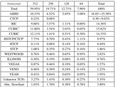
TABLE II

RESULTS OF WEB SERVERS WITH VALID TRACES

timeout 512 256 128 64 Total Total 59.95% 19.71% 12.71% 7.90% 100% AIMD 10.33% 6.52% 5.65% 3.08% 16.85∼25.58% CTCP 0.22% 0.08% 0.30∼9.03% BIC 9.68% 3.57% 1.11% 0.00% 14.36% CUBIC’ 11.60% 1.54% 2.03% 0.65% 15.82% CUBIC 12.11% 1.41% 0.51% 0.30% 14.33% HSTCP/CTCP’ 7.73% 0.70% 0.43% 1.11% 9.97% HTCP 0.11% 0.08% 0.14% 0.16% 0.49% STCP 1.08% 0.35% 0.27% 0.16% 1.86% WESTWOOD 0.76% 0.46% 0.65% 0.95% 2.82% ILLINOIS 0.30% 0.19% 0.08% 0.19% 0.76% VEGAS 0.87% 0.46% 0.19% 0.05% 1.57% VENO 0.46% 0.38% 0.24% 0.14% 1.22% YEAH 0.41% 0.84% 0.65% 0.05% 1.95% Unknown TCPs 3.27% 1.43% 0.38% 0.27% 5.35% Abn. SlowStart 1.03% 1.70% 0.38% 0.78% 3.89%

algorithms. The reasons for the remaining web servers are 1) a web server has a very short initial TCP timeout period, 2) CAAI could not establish a TCP connection to a web server, 3) CAAI does not receive any packet after establishing a TCP connection, 4) and other reasons.

For about 74% of web servers, CAAI successfully gathered valid traces as summarized in Table II. Recall that to achieve a high identification accuracy (described in Section IV-B), CAAI starts with timeout= 512 packets. If not successful, CAAI triestimeout= 256, 128, and finally 64 packets. Each column shows the information of web servers gathered with a timeout, and the last column shows the overall information. We can see that for 59.95%, 19.71%, 12.71%, and 7.90% of web servers with valid traces, CAAI successfully gathered congestion window traces with timeout = 512, 256, 128, and 64 packets, respectively. In the remaining part of this section, we consider only web servers with valid trace, and the percentage is calculated with respect to these web servers. Table II shows that overall only 16.85∼25.58% of web servers still use the traditional AIMD. The reason for the range is that whentimeout≤128 packets, it is very hard to distinguish between AIMD and CTCP. Therefore, for5.65%+ 3.08% = 8.73%of web servers, we do not know whether they use AIMD or CTCP. We can also see that overalla significant percentage (i.e.,14.36%+15.82%+14.33% = 44.51%) of web servers use BIC, CUBIC’, or CUBIC, and among these three TCP algorithms, CUBIC’ (i.e., the early version of CUBIC) has the largest number of web servers.

Surprisingly, Table II shows that a non-trivial percentage (i.e., 9.97%) of web servers use HSTCP. Figure 8 shows such an example. We manually checked the congestion window traces of these web servers, and we found that they are indeed very similar to HSTCP traces as shown in Figure 3(f) and quite different from CTCP traces as shown in Figure 3(c). For example, the congestion window sizes at RTT 35 in both Figures 8 and 3(f) are around 300 packets, whereas the congestion window sizes at RTT 35 in Figure 3(c) are around

(12)

93 93.5 94 94.5 95 95.5 96 1 4 16 64 256 1024 4096 16384 Identification Accuracy (%) Parameter W of CAAI

Fig. 6. CAAI achieves the best accuracy whenW_is around 256, and a very small or very bigW_impairs the identification accuracy.

80 85 90 95 100 0 0.01 0.02 0.05 0.1 0.2 0.5 1.0 2.0 5.0 Threshold RTT Accuracy (%)

Packet Loss Rate (%) CAAI EARLY WORK

Fig. 7. CAAI can very accurately detect the threshold RTT, and achieve much better accuracy than our early work [37].

Fig. 8. An early version of CTCP. Web Server in-dicated in HTTP headers: IIS/6.0, Operating System reported by NMAP [40]: Windows Server 2003.

Total No. of Emulated RTTs Network Environment A

Network Environment B

Fig. 9. A web server using YEAH. Web Server indicated in HTTP headers: CacheFlyServe v26b, Operating System reported by NMAP [40]: Linux.

Fig. 10. An unknown TCP algorithm. Web Server indicated in HTTP headers: Not Available, Operating System reported by NMAP [40]: Linux.

0 200 400 600 800 1000 1200 1400 0 5 10 15 20 25 30 35 Congestion Window (Pkts)

Fig. 11. Abnormal Slow Start. Web Server indicated in HTTP headers: uServ/1.53, Operating System reported by NMAP [40]: Linux.

390 and 300 packets. However, by manually checking their HTTP response header information, we found that most of these web servers use IIS 6.0 which runs on Windows Server 2003 or Windows XP Professional x64 Edition. Considering that Microsoft released a hotfix to add CTCP to these two Windows systems in 2008, we believe that these 9.97% of web servers may use an early version of CTCP (referred to as CTCP’), which behaves very similar to HSTCP but quite different from the latest CTCP in Windows Server 2008. We can see that overall 10.27∼19% of web servers use CTCP’ or CTCP, however, most of them still use the CTCP’ (i.e., the early version of CTCP).

Table II shows a small percentage of web servers use these non-default TCP algorithms (i.e., TCP algorithms other than AIMD, BIC, CUBIC, and CTCP). While some of them may be due to identification errors, we found that there are indeed some web servers using these non-default TCP algorithms. Figure 9 shows the traces of a web server using YEAH, which is almost the same as the traces of YEAH obtained on our local test-bed as shown in Figure 3(m). Surprisingly, there are also a non-trivial percentage (i.e., 5.35%) of web servers using some unknown TCP algorithms (i.e. not any of the 13 TCP algorithms). While some of them were due to bad network conditions between the CAAI computer and the web servers, we found that there are indeed quite a few web servers using some unknown TCP algorithms. Figure 10 shows such an example. Table II also shows that 3.89% of web servers have abnormal slow start (i.e., the slow start threshold after a timeout is higher than the congestion window size before the timeout). Figure 11 shows such an example.

Our preliminary CAAI measurement results, even though still not comprehensive, show a strong sign that the majority of TCP flows are not controlled by AIMD anymore (therefore, it is the time to reconsider the design goal of TCP-friendliness of new congestion control algorithms based on the majority of TCP algorithms), and a strong sign that the Internet congestion control has already changed from homogeneous to

highly heterogeneous (therefore, it is the time to reevaluate the performance and stability of the Internet based on the distribution of different TCP algorithms).

VIII. CONCLUSION

In this paper, we proposed a tool called CAAI for identify-ing the TCP algorithm of a remote web server, and presented our measurement results of the TCP deployment information of the 5000 most popular web servers.

There are still some limitations of the work described in this paper. The current CAAI does not consider some other TCP congestion control algorithms, such as FAST [53] which is not available in any operating system but has been used by some web servers, and does not consider XCP [54], VCP [55], and PERT [56], which have recently been proposed but not yet incorporated into any operating system. We plan to add the training feature vectors of more operating systems (e.g., FreeBSD, OpenBSD, Mac OS X, and Solaris) into our training set, so that we can more accurately identify their TCP algorithms. In addition, we plan to extend CAAI to actively identify the TCP algorithms of other types of Internet nodes (e.g., peer-to-peer nodes and FTP servers), and to identify the TCP algorithms of Internet flows in passively measured packet traces.

The current CAAI experiment covers only one IP address per web server and only 5000 web servers, which is still much less than the total number of web servers in the Internet. We plan to conduct more comprehensive measurements, and carefully investigate the web servers using non-default TCP algorithms, unknown TCP algorithms, and abnormal slow start algorithms.

ACKNOWLEDGMENT

The work reported in this paper is supported in part by NSF CAREER CNS-0644080 and NSF CNS-1017561.

(13)

REFERENCES

[1] V. Jacobson, “Congestion avoidance and control,” in Proceedings of ACM SIGCOMM, Stanford, CA, August 1988.

[2] D. Chiu and R. Jain, “Analysis of the increase/decrease algorithms for congestion avoidance in computer networks,”Journal of Computer Networks and ISDN, vol. 17, no. 1, pp. 1–14, June 1989.

[3] A. Tang, J. Wang, S. Low, and M. Chiang, “Equilibrium of hetero-geneous congestion control: Existence and uniqueness,” IEEE/ACM Transactions on Networking, vol. 15, no. 4, pp. 824–837, August 2007. [4] K. Munir, M. Welzl, and D. Damjanovic, “Linux beats Windows! -or the w-orrying evolution of TCP in common operating systems,” in Proceedings of PFLDNet, Marina Del Rey, CA, February 2007. [5] M. Weigle, P. Sharma, and J. Freeman, “Performance of competing

high-speed TCP flows,” inProceedings of NETWORKING, Coimbra, Portuga, May 2006.

[6] I. Rhee and L. Xu, “CUBIC: A new TCP-friendly high-speed TCP variant,” inProceedings of PFLDNet, France, February 2005. [7] K. Tan, J. Song, Q. Zhang, and M. Sridharan, “A compound TCP

approach for high-speed and long distance networks,” inProceedings of IEEE INFOCOM, Barcelona, Spain, April 2006.

[8] E. Kohler, M. Handley, and S. Floyd, “Datagram congestion control protocol (DCCP),”RFC 4340, March 2006.

[9] R. Stewart, “Stream control transmission protocol,”RFC 4960, Septem-ber 2007.

[10] G. Appenzeller, I. Keslassy, and N. McKeown, “Sizing router buffers,” inProceedings of ACM SIGCOMM, Portland, Oregon, August 2004. [11] D. Barman, G. Smaragdakis, and I. Matta, “The effect of router

buffer size on highspeed TCP performance,” inProceedings of IEEE GLOBECOM, Dallas, TX, November 2004.

[12] L. Xu, K. Harfoush, and I. Rhee, “Binary increase congestion control for fast long-distance networks,” inProceedings of IEEE INFOCOM, Hong Kong, March 2004.

[13] S. Ha, I. Rhee, and L. Xu, “CUBIC: A new TCP-friendly high-speed TCP variant,”ACM SIGOPS Operating System Review, vol. 42, no. 5, pp. 64–74, July 2008.

[14] S. Floyd, “HighSpeed TCP for large congestion windows,”RFC 3649, December 2003.

[15] R. N. Shorten and D. J. Leith, “H-TCP: TCP for high-speed and long-distance networks,” inProceedings of PFLDNet, Argonne, IL, February 2004.

[16] C. Caini and R. Firrincieli, “TCP-Hybla: A TCP enhancement for hetero-geneous networks,”International Journal of Satellite Communications and Networking, vol. 22, no. 5, pp. 547–566, September 2004. [17] S. Liu, T. Basar, and R. Srikant, “TCP-Illinois: A loss and delay-based

congestion control algorithm for high-speed networks,” inProceedings of VALUETOOLS, Pisa, Italy, October 2006.

[18] A. Kuzmanovic and E. W. Knightly, “TCP-LP: A distributed algorithm for low priority data transfer,” inProceedings of IEEE INFOCOM, San Francisco, April 2003.

[19] T. Kelly, “Scalable TCP: Improving performance in highspeed wide area networks,”ACM SIGCOMM Computer Communication Review, vol. 33, no. 2, pp. 83–91, April 2003.

[20] L. Brakmo, S. O’Malley, and L. Peterson, “TCP Vegas: New techniques for congestion detection and avoidance,” inProceedings of ACM SIG-COMM, August 1994, pp. 24–35.

[21] C. Fu and S. Liew, “TCP Veno: TCP enhancement for transmission over wireless access networks,” IEEE Journal on Selected Areas in Communication, vol. 21, no. 2, pp. 216–228, February 2003. [22] C. Casetti, M. Gerla, S. Mascolo, M. Y. Sanadidi, and R. Wang, “TCP

Westwood: Bandwidth estimation for enhanced transport over wireless links,” inProceedings of ACM Mobicom, Rome, Italy, July 2001. [23] A. Baiocchi, A. Castellani, and F. Vacirca, “YeAH-TCP: Yet another

highspeed TCP,” in Proceedings of PFLDNET, Los Angeles, CA, February 2007.

[24] Alexa Internet Inc., http://www.alexa.com/topsites.

[25] M. Allman, V. Paxson, , and W. Stevens, “TCP congestion control,” RFC 2581, April 1999.

[26] M. Allman, S. Floyd, , and C. Partridge, “Increasing TCP’s initial window,”RFC 3390, October 2002.

[27] N. Dukkipati, T. Refice, Y. Cheng, J. Chu, T. Herbert, A. Agarwal, A. Jain, and N. Sutin, “An argument for increasing TCP’s initial con-gestion window,”ACM SIGCOMM Computer Communication Review, vol. 40, no. 3, pp. 27–33, July 2010.

[28] S. Floyd, “Limited slow-start for TCP with large congestion windows,” RFC 3742, March 2004.

[29] S. Ha and I. Rhee, “Hybrid slow start for high-bandwidth and long-distance networks,” in Proceedings of PFLDNET, Manchester, UK, March 2008.

[30] M. Allman, V. Paxson, and E. Blanton, “TCP congestion control,”RFC 5681, September 2009.

[31] S. Floyd, T. Henderson, and A. Gurtov, “The NewReno modification to TCP’s fast recovery algorithm,”RFC 3782, April 2004.

[32] M. Mathis, J. Mahdavi, S. Floyd, and A. Romanow, “TCP selective acknowledgment options,”RFC 2018, October 1996.

[33] S. Floyd, J. Mahdavi, M. Mathis, and M. Podolsky, “An extension to the selective acknowledgement (SACK) option for TCP,” RFC 2883, July 2000.

[34] J. Padhye and S. Floyd, “On inferring TCP behavior,” inProceedings of ACM SIGCOMM, San Diego, CA, August 2001.

[35] J. Oshio, S. Ata, and I. Oka, “Identification of different TCP versions based on cluster analysis,” inProceedings of IEEE ICCCN, San Fran-cisco, CA, August 2009.

[36] S. Feyzabadi and J. Schonwalder, “Identifying TCP congestion control algorithms using active probing,” in Passive and Active Measurement Conference (PAM), Poster, Switzerland, April 2010.

[37] P. Yang, W. Luo, and L. Xu, “Towards measuring the deployment information of different TCP congestion control algorithms: The mul-tiplicative decrease parameter,” inProceedings of IEEE GLOBECOM, Miami, FL, December 2010.

[38] D. Comer and J. Lin, “Probing TCP implementations,” inProceedings of USENIX Summer Conference, Boston, MA, June 1994.

[39] A. Medina, M. Allman, and S. Floyd, “Measuring the evolution of transport protocols in the Internet,” ACM Computer Communications Review, vol. 35, no. 2, pp. 37 – 52, April 2005.

[40] Network Mapper (NMAP), http://nmap.org/.

[41] V. Paxson, “Automated packet trace analysis of TCP implementations,” inProceedings of ACM SIGCOMM, Cannes, France, September 1997. [42] Y. Zhang, L. Breslau, V. Paxson, and S. Shenker, “On the characteristics

and origins of Internet flow rates,” inProceedings of ACM SIGCOMM, Pittsburgh, PA, August 2002.

[43] S. Jaiswal, G. Iannaccone, C. Diot, J. Kurose, and D. Towsley, “Infer-ring TCP connection characteristics through passive measurements,” in Proceedings of IEEE INFOCOM, Hong Kong, March 2004.

[44] S. Rewaskar, J. Kaur, and F. Smith, “A performance study of loss detection/recovery in real-world TCP implementations,” inProceedings of IEEE ICNP, Beijing, China, October 2007.

[45] F. Qian, A. Gerber, Z. Mao, S. Sen, O. Spatscheck, and W. Willinger, “TCP revisited: a fresh look at TCP in the wild,” inProceedings of ACM IMC, Chicago, IL, November 2009.

[46] N. Seddigh and M. Devetsikiotis, “Studies of TCP’s retransmission timeout mechanism,” inProceedings of IEEE ICC, Helsinki, June 2001. [47] P. Sarolahti and A. Kuznetsov, “Congestion control in Linux TCP,” in Proceedings of the FREENIX Track: 2002 USENIX Annual Technical Conference, Berkeley, CA, June 2002.

[48] D. Wei, S. Hegdesan, and S. Low, “A burstiness control for TCP,” in Proceedings of PFLDNet, France, February 2005.

[49] P. Sarolahti, M. Kojo, K. Yamamoto, and M. Hata, “Forward RTO-recovery (F-RTO): An algorithm for detecting spurious retransmission timeouts with TCP,”RFC 5682, September 2009.

[50] HTTrack Website Copier, http://www.httrack.com/.

[51] PlanetLab, “An open platform for developing, deploying, and accessing planetary-scale service,” 2002, http://www.planet-lab.org/.

[52] S. Hemminger, “Network emulation with NetEm,” inProceedings of the 6th Australia’s National Linux Conference, Australia, April 2005. [53] C. Jin, D. X. Wei, and S. H. Low, “FAST TCP: motivation, architecture,

algorithms, performance,” in Proceedings of IEEE INFOCOM, Hong Kong, March 2004.

[54] D. Katabi, M. Handley, and C. Rohrs, “Internet congestion control for high bandwidth-delay product networks,” inProceedings of ACM SIGCOMM, Pittsburgh, August 2002.

[55] Y. Xia, L. Subramanian, I. Stoica, and S. Kalyanaraman, “One more bit is enough,” inProceedings of ACM SIGCOMM, Philadelphia, PA, August 2005.

[56] S. Bhandarkar, A. Reddy, Y. Zhang, and D. Loguinov, “Emulating AQM from end hosts,” in Proceedings of ACM SIGCOMM, Kyoto, Japan, August 2007.