Data Assimilation in the Solar Wind: Challenges and
First Results
Matthew Lang1,Philip Browne2,3,Peter Jan van Leeuwen2,4, Mathew Owens2
Matthew Lang, [email protected]
1Le Laboratoire des Sciences du Climat et de l’Environnement, CEA-CNRS-UVSQ, 91191 Gif Sur Yvette, France
2Department of Meteorology, University of Reading, Reading, Berkshire, UK
3Currently at European Centre for Medium-Range Weather Forecasts, Reading, Berkshire, UK
4NCEO, University of Reading, Reading, Berkshire, UK
This article has been accepted for publication and undergone full peer review but has not been through the copyediting, typesetting, pagination and proofreading process, which may lead to differences
be-Abstract. Data Assimilation (DA) is used extensively in numerical weather prediction (NWP) to improve forecast skill. Indeed, improvements in fore-cast skill in NWP models over the past 30 years have directly coincided with improvements in DA schemes. At present, due to data availability and tech-nical challenges, DA is underused in space weather applications, particularly for solar wind prediction. This paper investigates the potential of advanced DA methods currently used in operational NWP centres to improve solar wind prediction. To develop the technical capability, as well as quantify the po-tential benefit, twin experiments are conducted to assess the performance of the Local Ensemble Transform Kalman Filter (LETKF) in the solar wind model ENLIL. Boundary conditions are provided by the Wang-Sheeley-Arge coronal model and synthetic observations of density, temperature and mo-mentum generated every 4.5hr at 0.6AU. While in-situ spacecraft observa-tions are unlikely to be routinely available at 0.6AU, these techniques can be applied to remote sensing of the solar wind, such as with Heliospheric Im-agers or Interplanetary Scintillation. The LETKF can be seen to improve the state at the observation location and advect that improvement towards the Earth, leading to an improvement in forecast skill in near Earth space for both the observed and unobserved variables. However, sharp gradients caused by the analysis of a single observation in space resulted in artificial wave-like structures being advected towards Earth. This paper is the first attempt to apply DA to solar wind prediction, and provides the first in-depth analysis of the challenges and potential solutions.
Keypoints:
• The paper describes the first data assimilation (DA) experiments with a solar wind model.
• These experiments show that DA can improve forecasts of non-magnetic variables near the observation, which are advected by the solar wind.
• We discuss challenges and obstacles inherit to DA in the solar wind and propose potential solutions as directions for future research.
1. Introduction
Variability in the solar magnetic field over minutes, hours and days results in near-Earth solar-wind conditions which can adversely affect space- and ground-based tech-nologies [Cannon et al., 2013]. The most extreme “space weather” is driven by Coronal Mass Ejections (CMEs), large episodic eruptions of plasma and magnetic field from the Sun that travel through the solar wind, disturbing the Earth’s magnetic field as part of a geomagnetic storm [Gosling, 1993]. As such, Earth-directed CMEs pose a threat to electrical and communication systems which have become a huge part of modern-day life, with an estimated potential economic impact of up to $2 trillion in the first year after an extreme storm [Board, 2008]. In addition, the radiation hazard of energetic charged particles associated with the solar wind and by CMEs is a health threat to humans at high altitude, such as aircrew over the poles and astronauts, both in low-Earth orbit (e.g., on the International Space Station), but particularly on interplanetary missions, when the protection of the Earth’s magnetic field is removed [Cannon et al., 2013]. The UK has responded to the danger of a major space weather event, such as a large CME, by adding it to the National Risk Register as one of the largest threats to modern society. The UK Met Office (UKMO) and US Space Weather Prediction Center (SWPC) are working to-gether to prepare for, and mitigate against, the possible impacts of a large space weather event. Thus forecasting solar wind conditions in near-Earth space is a high priority.
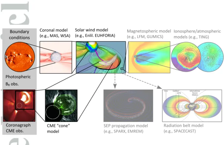
The state-of-the-art method for forecasting near-Earth solar wind conditions is through coupled coronal and heliospheric models, with boundary conditions ultimately set by photospheric magnetic field observations (e.g., see Figure 1). As a complete photospheric
magnetic field map takes one solar rotation to construct ( 27 days from Earth’s point of view), this approach enables the quasi steady-state solar wind to be predicted. Time-dependent phenomenon, such as CMEs, are then incorporated through ad-hoc perturba-tion of heliospheric boundary condiperturba-tions. This typically entails a “cone model” which inserts an over-pressurised density perturbation with the speed, direction and angular width set by coronagraph observations of the CME in question (for example, see [Parsons et al., 2011; Xie et al., 2004]). No additional observational constraints are imposed on the forecast between the top of the solar corona ( 20 solar radii) and near-Earth space ( 215 solar radii). For operational solar wind forecasting, UKMO and SWPC use ENLIL [Parsons et al., 2011; Odstrcil and Pizzo, 1999; Odstrcil et al., 2004;Odstrcil, 2003], a 3D
magnetohydrodynamic (MHD) model.
In this paper, we investigate the use of an advanced data assimilation method with the ENLIL model for potential improvement of space-weather forecasting. To the authors’ knowledge, this is the first study to apply data assimilation methods to the solar wind. We use the EMPIRE [Browne and Wilson, 2015] data assimilation framework. In the next section the solar wind is described. Then the basic ingredients are described in succession, a short introduction to data assimilation, the model ENLIL, and the EMPIRE data-assimilation framework. This is followed by the set up of the data-assimilation experiments and the results, and a concluding section.
2. The solar wind
The solar wind is a plasma composed primarily of electrons and protons, with a small contribution from alpha particles and other minor species. It continually flows almost
the heliosphere. The mechanism(s) by which the corona is heated, however, are still debated (e.g.,De Moortel and Browning [2015]), as are the precise mechanism(s) by which the coronal plasma is confined and released [Cranmer, 2008; McComas et al., 2007]. The solar wind drags the coronal magnetic field outwards generating the heliospheric magnetic field (HMF [Owens and Forsyth, 2013]), which magnetically couples the Sun and planets, and modulates the flux of galactic cosmic rays in the inner heliosphere. The solar wind plasma is accelerated to speeds greater than the characteristic wave speeds (i.e., the local Alfven and fast magnetosonic wave speeds) within 0.1 AU (where 1AU ≈ 1.50×10⁸km is the astronomical unit, defined as the average distance between the Earth and Sun), meaning that no information from the solar wind beyond this distance can propagate back towards the Sun. Typical properties of the solar wind at 1AU are summarised in table 1.
The ambient solar wind has two distinct components, typically referred to as the “fast” (∼ 750kms−1) and the “slow” solar wind (∼ 400kms−1), although their differences are not limited to only their speed (and extend to their formation mechanism at the Sun, for example). Fast solar wind flows outwards along “open” magnetic field lines associated with coronal holes [Hassler et al., 1999], which are largely confined to the polar regions at times around sunspot minimum. The slow solar wind emanates from, or regions close to, closed coronal loops, which are confined to equatorial regions at sunspot minimum. During solar maximum, the coronal magnetic field is far more dynamic, with a much weaker dipole component. Consequently, the slow solar wind is observed at a much greater range of solar latitudes.
In-situ spacecraft observations of the solar wind provide direct measurements of the solar wind plasma and HMF, which is directly rebateable to state vectors of the ENLIL simulation. However, only sparse spatial coverage of the global heliosphere is possible. Temporally, there has been near-complete data coverage in near-Earth space since 1996. Close to theL1 Lagrangian point between the Sun and the Earth (at heliocentric distance of ∼0.99AU), ACE [Stone et al., 1998] and Wind [Gloeckler et al., 1995] spacecraft have provided measurements since 1996, with the DSCOVR mission [Leslie and Cole, 2016;
Burt and Smith, 2012] taking over as the standard observatory in June 2015. Away from near-Earth space, the two STEREO spacecraft [Kaiser et al., 2008; Davis et al., 2009] observe the solar wind from the elliptic plane, drifting 22◦ further ahead and behind the Earth each year, and the HELIOS spacecraft [Jackson, 1985a, b] which explored the inner heliosphere to 0.29AU. This data is all freely available online (e.g. at
https://nssdc.gsfc.nasa.gov/space/).
From the available data it is difficult to forecast the near-Earth solar wind directly. Photospheric extrapolation enables a quasi-synoptic estimate of the near-Sun solar wind conditions, but it is highly indirect and therefore subject to large uncertainties. The sparse in situ observations are more reliable, but sample only a small region of space; the L1 point is too close to Earth to provide a useful forecast lead time, and there are only extremely infrequently ”upwind” monitors on the Earth-Sun line (e.g., the HELIOS spacecraft for very short intervals during the late 1970s and early 1980s). Heliospheric Imager (HI) type instruments, such as those on board STEREO [Eyles et al., 2009], and Interplanetary Scintillation (IPS) measurements [Manoharan and Ananthakrishnan, 1990] enable greater spatial sampling solar wind for limited properties (primarily density, but also solar wind
speed). Interpretation of these observations requires deconvolution of geometrical and path-integrated effects, thus there is large uncertainty in, e.g., solar wind speed, at a given point in the heliosphere. This is where data assimilation can be of assistance because it incorporates a full dynamical model of the solar wind, to some extent interpolating the observations to obtain a more complete picture, and allows for observational and model uncertainty. Thus it provides a natural starting point for prediction. Here, we explore how these observations can be brought together. We use a solar wind model (ENLIL) initiated using the near-Sun solar wind conditions from photospheric magnetic field observations, and assimilate solar wind conditions at a single point, located 0.6 AU along the Sun-Earth line. In the remainder of the study, we consider these solar wind observations to be synthetic in-situ spacecraft observations, but they could equally represent HI or IPS observations.
3. Short introduction to Data Assimilation
Data assimilation combines prior information of a system encoded in a numerical model with new observational information to obtain a better description of the evolution of that system, including uncertainty estimates. The information in each component is represented by a probability density function (pdf). Data assimilation is based on Bayes Theorem, which tells us that the prior pdf of the model has to be multiplied with the pdf of the observations to obtain the posterior pdf of the model given the observations:
p(x|y) = p(y|x)
p(y) p(x) (1)
in which xdenotes the model, and y the observations, and the functions p(..) denote the different pdfs, distinguished by their arguments. The model x can be the state of the
model at a specific time or a model trajectory over a certain time window. Similarly, the observations y can denote observations at a specific time, or over a set of observations over a certain time window. Ifx is the model state at a specific time and y only contains observations at or before that time, it is referred to as filtering, while smoothing refers to the situation that y contains observations that occur at a later timestep than x, and x
can be a state or a trajectory over time. If x and y refer to different times the Bayesian framework needs the joint pdf of the state,x, and the state at the time of the observation to bring the observation information to the state, x, at the time of interest. Details can be found in the literature and at the end of this section.
The state of the model is described by a state vectorx∈RNx, which contains the values
of the quantities of interest at all gridpoints, whereNx is the dimension of the state. For
ENLIL, the state vector contains the three components of the magnetic field vector, the three components of the solar wind plasma momentum vector, the plasma temperature, the plasma density and the cloud and polarity tracers, at each grid point of the model.
The evolution of the model is described by the model equation
xi+1 =fi(xi) +ηi (2)
where xi is state vector at timestep i, fi represents the pure model that incorporates
our understanding of the physics of the system, and ηi is an Nx-dimensional stochastic
term that represents the error in the model equations, resulting from discretisation errors, missing physics and inaccurate boundary conditions. In the case of solar wind forecasting, the inaccurate boundary conditions are expected to be the largest single factor. In data assimilation the statistics of the model errors is assumed to be known, e.g., Gaussian with
mating these statistics is becoming an active field of research in e.g., weather prediction, where, traditionally, these model errors have been ignored for computational reasons.
In the geosciences we never know the initial state vector, and in data assimilation it is typically assumed to be a random perturbation from the true state:
xb =xt0+ξ0 (3)
where xb ∈ RNx is the initial state, xt
0 ∈RNx is a discretisation of the true state at time 0, and ξ0 ∈ RNx represents the random error in the initial state. Since the truth is not known the initial condition is either based on a previous forecast or is carefully generated using all physical knowledge at hand.
The observations are measurements of the true system, but contain measurement er-rors. They also contain errors arising from the fact that model and observations tend to represent reality differently, e.g. they have different spatial resolution. Quantifying these so-called representation errors is again an active area of research, see e.g. Hodyss and Nichols [2015] and van Leeuwen [2015]. The relation between observations and state of the system is written as:
yi =Hi(xti) +i (4)
where Hi :RNx → RNy, the observation operator, maps the state into observation space
and Ny is the dimension of the observations. The observation error, containing both
instrument and representation error is given by i, the statistics of which we assume to
be known.
Data assimilation can be used for state estimation, as described above, but it is also used for parameter estimation, see e.g. [Smith et al., 2009; Evensen et al., 1998] and
has recently being applied to the estimation of non-linear parameterisations [Lang et al., 2016]. In this paper, however, we shall focus upon state estimation.
It is important to realise that there is a fundamental problem in data assimilation for the geosciences that has to do with the size of the problems involved. Suppose we want to store the prior pdf of a 100-dimensional system, which is a relatively small system. Since that pdf can have any shape we would have to rely on histogram representations. Assume we use 10 frequency bins for each variable, then we need to store of the order of 10100numbers. Our present-day supercomputers can store a lot of numbers, but this is completely out of the question. By comparison, the number of atoms in the observable universe is estimated to be of the order of 1080, so the data-assimilation problem is larger than the observable universe! =This estimate is very conservative, the dimension of the state vector for the low-resolution ENLIL simulations performed in this study is 3,888,000. This means that one has to make approximations to the full bayesian solution, and a large part of data-assimilation research is focussed on finding the best approximation for specific problems. This has resulted in a number of different data assimilation methods, and the following gives a very brief overview of what is currently used in the geosciences. More detailed information can be found in recent text books like Nakamura and Potthast [2015], Reich and Cotter [2015], and van Leeuwen et al. [2015].
3.1. Variational methods
While variational methods are not used in this paper, for reasons discussed below, it is useful to give an overview of the approach.
In variational methods one tries to find the mode of the posterior pdf, so the most probable state of the model given the observations. The mode is defined as
ˆ
x=argmaxx p(x|y). (5)
Writing p(x|y) = exp[−J(x)], this amounts to minimising the cost function J, which is done by setting the gradient of that function to zero and deriving the Euler-Lagrange equations, and solving these with an efficient gradient descent algorithm, such as conjugate gradient. This involves generating the tangent-linear model and its transpose, the adjoint, of the nonlinear model code, which can be a formidable task.
As an example, when we assume Gaussian errors statistics with zero means and covari-ances; Rk for observational errors, B for initial condition errors, and Qi for model errors we find this cost function:
J (XNt) = 1 2 x0−x bT B−1 x0−xb+1 2 d X k=1 h (Hk(xik)−yk) T R−k1(Hk(xik)−yk) i + 1 2 N−1 X i=0 h (xi+1−f(xi))T Qi−1(xi+1−f(xi)) i . (6) whereXNt = (x0, . . .xNt) T
is the vector of the states at all timesteps, Nt, and ik denotes
the time steps that we have observations in the time window. Minimising this cost function is the so-called Weak Constraint 4DVar problem; 4D because it contains space and time, and weak-constraint because it allows for errors in the model equations. When these are ignored, the last term is absent and we obtain Strong Constraint 4DVar.
For numerical weather prediction, and also for space weather applications, the covari-ance matrices involved are huge, e.g. 1018 for weather prediction, so they cannot be stored explicitly, and are coded as operators working on input vectors. Furthermore,
strong-constraint 4DVar the matrix B is often used, and it is still unclear what the best preconditioning is for the weak-constraint 4DVar.
3.2. Ensemble Kalman Filters
While variational methods are very powerful they have a few major drawbacks. The first one is that coding up the tangent linear and adjoint of the nonlinear forward model is a serious exercise, and for a complex model like ENLIL, this could easily take up a person year or more. Furthermore, when the problem is highly nonlinear the posterior pdf can have multiple modes, and finding the global mode is not trivial. Finally, when the initial state errors are not Gaussian standard optimisation methods cannot be applied and very little experience is available in the community.
An alternative are sequential methods, that forecast the initial state,xb, and its uncer-tainty to the first observation timestep, i0, using the numerical model. Bayes Theorem is used to update the pdf, and a new forecast is made to the next observation. The ma-jority of sequential methods are based upon the Kalman Filter [Kalman, 1960; Kalman and Bucy, 1961]. Kalman Filter-based methods search for the minimal variance state, so the mean of the posterior pdf. They assume that all pdfs are Gaussian, so only the mean and the covariance are needed to describe all pdfs involved. The main advantage of the approach is that a sequential method is typically simpler to implement and does not require the computation of the adjoint of the forward model. The Kalman Filter also explicitly evolves the forecast state covariance matrix, Pf, through the assimilation window. However, this requirement also renders the Kalman Filter impractical for use in high dimensional systems, as it may not be possible to explicitly store the forecast state
To solve this issue, the pdf is represented by a number of samples or ensemble members, and these are propagated to observation times using the full nonlinear model equations. At the observation time, the Kalman filter equations for updating mean and covariance are used to define the posterior pdf, using the ensemble members to provide prior estimates for them. By using the fact that the number of ensemble members is typically much smaller than the system dimension, very efficient updating schemes have been developed. This has resulted in a large class of so-called Ensemble Kalman Filters (EnKFs), a set of Monte-Carlo based sequential DA methods.
There are two main issues that hinder application in high-dimensional geophysical sys-tems. Firstly, due to the small ensemble size M, typically in the range 10−500, which is much smaller than the system dimension, Nx, the ensemble covariance matrix has rank
M −1, which is much smaller than full rank. It spans only the directions of the ensem-ble perturbations from the ensemensem-ble mean, and hence the covariance is estimated from below. To compensate for this under estimation (and typically also to compensate for an under-representation of the model errors), covariance inflation is applied. There are sev-eral ways to do this, and the most widely used method is simply multiplying the ensemble covariances by a factor 1 +ρ >1, as follows:
˜
Pfinfl = (1 +ρ)P˜f (7)
in which Pf is the forecast ensemble at the observation time and P˜finfl represents the in-flated forecast error covariance matrix. This multiplication has the effect of increasing the spread in the forecast ensemble to better represent the true errors in the model. However, the uncertainty is only increased in the directions already covered by the ensemble. Other
methods for covariance inflation have been developed, see e.g. [Anderson, 2007] for an overview.
The second issue is that the covariances are estimated directly from a rather small ensemble, so especially small covariances are prone to sampling noise. Since covariances are expected to be small between distant grid points, so-called covariance localisation can be applied, in which the sample covariance is multiplied, via a Schur product, with a localisation matrix that tapers off quickly with gridpoint distance [Houtekamer and Mitchell, 2001]. This procedure ensures that the spurious correlations between points are reduced and hence unrealistic covariances do not affect the analysis of the state. Another advantage of localisation is that it makes the ensemble covariance matrix more diagonal, resulting in a localised ensemble covariance matrix that is, typically, of higher rank.
However, as mentioned before, the ensemble covariance is never calculated explicitly as it would not fit in memory leading to a different localisation strategy called obser-vation localisation. In this method each grid point is treated separately by selecting a localisation radius and only observations within that radius are allowed to update this gridpoint. Within the localisation radius the observation covariance matrix is multiplied with a factor increasing with the distance of the observation to the gridpoint, so that observations further away have a larger error, and hence have less effect on the update of that gridpoint. This ensures a smooth spatial update. It is important to realise that inflation and localisation are essential ingredients in Ensemble Kalman Filtering.
In this study, we shall use the LETKF, as developed by [Hunt et al., 2007], which uses observation localisation. The LETKF is one of the most efficient and accurate methods currently used in operational weather prediction centres, such as the Japanese
Meteoro-logical Agency (JMA) [Miyoshi et al., 2010] and the National Center for Environmental Prediction (NCEP) [Szunyogh et al., 2008]. Appendix A contains a description of the full LETKF algorithm, showing how the whole algorithm works very efficiently in the low-dimensional ensemble space.
3.3. Other data assimilation algorithms
Recent years have seen a surge of other Monte-Carlo-based methods for geophysical problems, mainly particle filters. Their main advantage over the methods discussed above is that they are fully nonlinear. However, until recently these methods were thought to be too inefficient to be useful in high-dimensional systems. But by exploring either the proposal density freedom or localisation, efficient algorithms have been developed that are very promising for high-dimensional geophysical problems (see recent overviews in Reich and Cotter [2015] and van Leeuwen et al. [2015]).
Another active area of research is in hybrid methods, where different data-assimilation methods are combined, exploiting the strengths of each. Examples are ensemble smoothers like 4DEnsVar, in which an ensemble of model runs is used to generate space-time covari-ances that alleviate the need for tangent linear and adjoint models in a 4DVar algorithm. We will not discuss these developments here but refer to recent papers likeFairbarn et al.
[2014],Goodliff et al. [2017] and Amezcua et al.[2017] and references therein.
4. The ENLIL heliospheric solar wind model
The dynamics of the solar wind differ from the typical dynamics of the atmosphere, as the solar wind is strongly driven by the conditions at the top of the corona (i.e., the inner boundary condition to the ENLIL model), whereas typical atmospheric systems are
highly chaotic, so very sensitive to small perturbations. This has direct consequences for the data assimilation, as we will see later.
Over time and length scales greater than the electron and ion gyromotions, which are many orders of magnitude below typical solar wind model resolutions, the large scale behaviour of the solar wind plasma can be well respresented as a magnetised fluid, the magnetohydrodynamic (MHD) approximation. Under such conditions, the fluid has neg-ligible resistivity and so can be treated as a perfect conductor. This means that, through Lenz’s law, the motion of the plasma and the magnetic field is “frozen” together; as long as resistivity remains negligible, the magnetic field within the plasma of the solar wind will move with the velocity of the plasma e.g., Kivelson and Russell [1995]. Ideal MHD, the simplest approximation of MHD, therefore reduces to the continuity equation, the Cauchy momentum equation, Amp`ere’s Law and a temperature evolution equation. Thus ideal MHD explicitly represents the conservation of mass, momentum, total energy and induction of the magnetic field, as well as the effects of the magnetic field via magnetic field pressure and tension of magnetic field lines [Odstrcil, 2004] (the force exerted by the curvature in a magnetic field line as it tries to “straighten” out).
The ENLIL model is a 3D numerical model that is used operationally at the UK Met Office and NOAA’s Space Weather Prediction Centre in combination with coronal models and magnetospheric models, as described in figure 1. It is based upon the ideal mag-netohydrodynamics (MHD) equations, with two additional continuity equations for the ‘Cloud Tracer’, a passive tracer that traces the material from a cone-model CME, and the ‘Polarity Tracer’, a passive tracer for the polarity of the HMF (seeOdstrcil and Pizzo
at run time, in order to avoid the HMF numerically diffusing away close to the polarity inversion (i.e., the heliospheric current sheet). It is then returned to its bipolar state post-run. Numerical calculations are performed in a spherical coordinate system on a do-main decomposition approach to divide the 3D computational dodo-main into smaller radial slabs for processing on parallel systems, via MPI (Message Passing Interface)[Gropp et al., 1996]. Each processor then solves the MHD equations on the respective radial slabs and boundary data for each slab is exchanged via MPI calls.
The inner boundary of the ENLIL model is specified at ∼ 0.1AU, outside the point at which the solar wind becomes supersonic. Thus there is no sunward propagation of information through the inner boundary, simplifying the numerical computation. To specify the inner boundary conditions, the Wang-Sheeley-Arge (WSA) model [Wang and Sheeley Jr, 1992;Arge and Pizzo, 2000], a semi-empirical model of the corona, is typically used. The WSA model takes observations of photospheric magnetic field as input and extrapolates the field through the corona, typically to a source surface of around 2.5 solar radii, using the potential-field source-surface approximation. The solar wind velocity, proton density and temperature can be derived using empirical relationships to the coronal magnetic field, assuming a constant mass flux (seeLopez [1987] and Riley et al.[2015] for more details). These properties are radially mapped to 0.1AU (ENLIL’s inner boundary). All of these structures are rotating, with an azimuthal velocity equal to the Sun’s rotation speed along the inner boundary to create the inner boundary values for all time steps in the time domain.
5. The EMPIRE data assimilation system
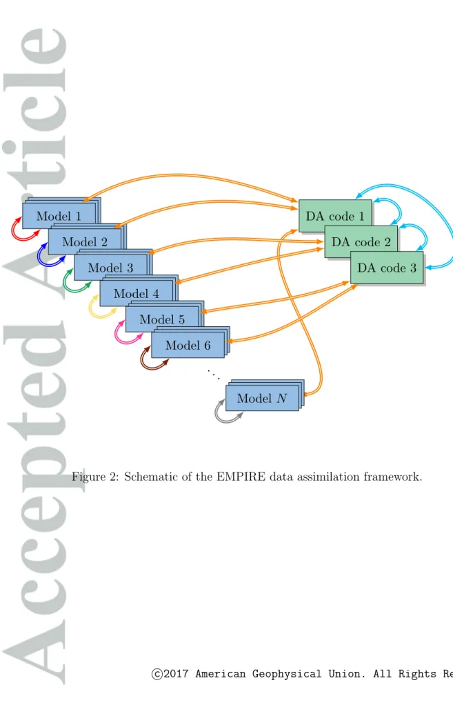
To perform the data assimilation experiments efficiently, the EMPIRE data assimilation system [Browne and Wilson, 2015] is used. EMPIRE contains data assimilation codes that link to the model via a small number of MPI commands [Gropp et al., 1996], see Figure 2 for a visualisation of this. The data assimilation methods in EMPIRE include some of the most advanced ensemble-based data assimilation methods such as the LETKF (which shall be used in this paper), the Bootstrap Particle Filter, the Equivalent Weights Particle Filter, the Implicit Equal Weights Particle Filter and 4DEnVar. The codes have been optimised to run in parallel, via MPI commands, such that large ensembles can be processed efficiently and effectively. At observation time, the model passes a state vector to EMPIRE which performs the data assimilation independent of the model, and then passes the analysed state vector back to the model and waits until the next observation timestep.
There are other data assimilation libraries available such as the Data Assimilation Re-search Testbed (DART) [Anderson et al., 2009] and Parallel Data Assimilation Framework (PDAF) [Nerger et al., 2005]. While these data-assimilation systems are highly optimised their main strength is that they are focussed on academic users. This means that min-imal coding is needed to couple any numerical model to these systems, exploring the fact that most ensemble-based data-assimilation methods are not dependent on how the model works. Furthermore, once coupled it is extremely easy to switch data-assimilation method, allowing fast comparisons and a fast way to choose the best method for the prob-lem at hand. Additionally, EMPIRE and PDAF have the additional advantage that it is not necessary for the model to write to disk every assimilation step, due to the efficient
use of MPI and/or subroutine calls, meaning more efficient computations. Moreover, all these systems are community code with active user support.
As the DA codes are completely general, it is necessary to specify the observation timesteps, the observation operator, the error covariance matrices and distances between two points in the state vector (for the LETKF) only. This makes the implementation of EMPIRE into the numerical model relatively simple in comparison to DART, which require the model code to be adjusted to a higher degree than the simple MPI command required for the implementation of EMPIRE [Browne and Wilson, 2015].
6. Numerical experiments
Since this paper describes initial tests of a data-assimilation experiment we perform the experiments in a controlled way. We start by recognising that we have some uncertainty in the model state. With this uncertainty we are able to generate an ensemble which represents our prior pdf. Then, using the same technique as we use to generate each ensemble member, we generate one further model state which we refer to as the truth
state. We use our numerical model to propagate this truth state to get a complete truth trajectory. We then take artificial observations from a fixed point in space from this truth trajectory. These ‘observations’ are perturbed by measurement noise to mimic a real data assimilation experiment. The goal is to closely represent the posterior pdf, which represents the best estimate including an uncertainty estimate of the truth run, using the limited information from the observations and uncertain prior information on initial and boundary conditions. The ensemble generated is evolved using the numerical model in two seperate runs, one with data assimilation performed and one without it to evaluate
the performance of the data assimilation scheme used. This set up is called an identical twin experiment, and it is the first test for any data-assimilation system.
6.1. Experimental setup
Twin experiments have been performed using the LETKF to assimilate observations of the true state generated from an unknown initial condition.
The state vector for the solar wind field is defined as a vector of the density, temperature, momentum (radial, latitudinal and longitudinal components), the magnetic field (radial, latitudinal and longitudinal components) and cloud and polarity tracers at each point in the ENLIL domain. Writing this mathematically:
x=ρT,TT,(ρvr) T ,(ρvθ) T ,(ρvφ) T ,BrT,BθT,BφT,ρcT,ρpT T (8)
where the bold-font denotes the relevant variable at all radial, latitudinal and longitudinal point in the model’s domain.
ENLIL is run with an inner boundary of 0.1AU and outer boundary of 1.1AU in a spherical grid with 144 radial points equally spread throughout the domain; 30 latitudinal points spread equally between 30◦−150◦ latitude (with 0◦ defined as the north pole of the Sun) and 90 longitudinal points spread equally between−90◦ and 90◦ with 0◦ defined as the line between the Sun and Earth. The time domain is 5 days with time steps every 320 seconds (plus an additional spin-up time of∼5.93days).
6.1.1. Assimilation parameters
Boundary conditions for ENLIL were generated at 20 solar radii (≈0.1AU) from outputs of the WSA model for a magnetogram from 01/04/2013. To generate the truth run, the ENLIL model was spun-up for 5.12×10⁵s(1600 timesteps or≈5.93 days) in order for the
inner boundary conditions to advect the solar wind structures through the whole model domain. These spun-up boundary conditions are then used as initial conditions for the data assimilation experiments. By spinning up the boundary conditions in this manner, as opposed to prescribing a set of initial conditions (from a long run, for example), we avoid initialisation shocks occurring in the domain that may contaminate our results. The truth run started after spin up and lasted for 5 days, using 1350 model time steps.
Observations of the true state were taken every 50 timesteps (approximately every 3 hours). The observations were taken of density, temperature and the momentum variables with an observation error covariance given by the diagonal matrix,R ∈R5×5, where the variances along the diagonal are shown in Table 2. The variances are approximately 1−10% of typical variable values at the observation location. In the experiments shown here, observations are taken at a single point (to represent a spacecraft, or properties at a single point in space determined from HI or IPS observations) in the ecliptic plane between the Earth and Sun. Observations are taken in the middle of the ENLIL domain, at approximately 0.6AU. This was not done near the Earth (at 0.99AU), as would be most realistic at the present, as this is close to ENLIL’s outer-boundary and hence it could be not seen how the LETKF affected the state downwind. It is worth noting at this point, that after launch in 2019, ESA’s Solar Orbiter and NASA’s Solar Probe Plus will be taking observations of the solar wind at a radius of approximately 0.3AU. While such observations will not be routinely available for forecasting, they will enable both more direct testing of the DA schemes and calibration of the near-Sun HI and IPS observations. Two ensemble runs were used, a model-only ensemble run without data assimilation, and an ensemble run where we use the LETKF. The model-only ensemble run represents
the propagation of the prior pdf in time. By studying how the LETKF ensemble deviates from that pdf evolution we can infer the impact of the data assimilation.
Our initial attempt at creating an ensemble was by adding random perturbations to the inner boundary condition generated from a diagonal initial error covariance matrix to an initial state generated using the WSA model boundary condition but found this to be ineffective [Lang, 2016]. The spread ensemble was too small, and simply increasing the magnitude of this diagonal covariance matrix, causing the ENLIL model to become numerically unstable. Ideally, a covariance matrix that has proper correlations between all model variables should be used, but generating such a matrix is rather complicated and needs very long model runs. In NWP, the specification of such a covariance matrix can form a substantial part of the scientific effort to improve the state estimation.
Instead, here we use an ensemble of 48 members generated from snapshots of a long model run. Boundary conditions were drawn from 48 random WSA model outputs from the year 2015 (so they are independent from the true state). The random selection of the boundary conditions is done in order to ensure a wide variety of the Sun’s behaviour, both in terms of phasing of structures with solar rotation and changes in the patterns of the solar wind (e.g.slow/fast wind). Like the truth run, each ensemble member was spun up for 1600 time steps to avoid initialisation shocks. This effectively swept out the model interior from the snapshots of the long model run, and left us with internally balanced initial model states consistent with the boundary conditions.
Once the initial ensemble was specified from the boundary conditions, as described as above, the model-only ensemble was generated by propagating the 48 ensemble members through time to the end of the assimilation window of 5 days with 1350 timesteps, with
no data assimilation. Using the same initial ensemble as the model-only ensemble, the LETKF was used to perform data assimilation experiments.
As mentioned previously in the data assimilation methods section, a localisation func-tion must be specified. In order to avoid upwind informafunc-tion propagafunc-tion from the obser-vation location back towards the Sun, an asymmetric radial distance-based localisation function has been specified. Downwind of the observation location a truncated Gaussian function centred on the observation location was used with localisation radius of 0.01AU. Upwind of the observation the localisation function is set to 0. Here this localisation function multiplies the observation error covariance matrix, R−1. That is to say, the localisation function only allows points within a radius of ∼ 0.04 AU downwind of the observation to be updated and no points upwind of the observation to be influenced by the observation.
The experiments shown in this paper were run on 1176 processors on ARCHER [http://www.archer.ac.uk/, 2017], the UK national supercomputing facility. Each pro-cessor has all variables at all latitudes and longitudes in the computational domain with 8 radial points, the first and last radial values shared with the previous and next processor via MPI, respectively.
6.2. Diagnostics
In the following sections, for visualisation purposes, the variables are multiplied by a factor of r2, the distance to the sun squared, to compensate for the r2 decrease in density, momentum and magnetic variables away from the Sun. This allows us to easily see structures in the state propagating further into the domain.
Results are analysed over the ecliptic plane (i.e. the plane containing the Earth and the Sun) only. Results from the LETKF are sampled every 10 timesteps. The radial points,
r = 2,10, . . . ,138, are sampled every 8 gridcells (every ∼ 0.0056AU), the latitudinal coordinate is taken at onlyθ = 90◦, and longitudinal coordinates,φ=−40◦,−30◦, . . . ,40◦, are sampled every 10◦ around the Earth-Sun line.
The absolute error is also calculated at the observation point for the model-only ensem-ble and LETKF analysis ensemensem-ble mean. This absolute error, or RMSE, in the ensemensem-ble at the observation point is calculated by:
|xtr,φ−xr,φ| (9)
where xt
r,φ is the true state for a single variable at the point (r, φ) in the spatial domain,
xr,φ = M1 PM m=1 xm r,φ
is the ensemble mean for either the LETKF or model-only ensemble at a single point (r, φ) and xmr,φ is the mth ensemble member at (r, φ).
The ensemble spread at each coordinate is also generated by calculating the standard deviation of the respective ensemble at each radial and longitudinal point, which is given by: v u u t 1 M−1 M X m=1 h xm r,φ−xr,φ 2i . (10)
The differences between the absolute errors for the LETKF and model-only ensemble are also calculated, at each point in the ecliptic plane sampled (for each (r, φ) point in equation (9)), as |xtr,φ−xsto r,φ| − |x t r,φ −xar,φ| (11) where xsto
r,φ represents the model-only ensemble mean and xar,φ represents the LETKF
There-fore, positive values (red regions on polar plots) indicate an improved LETKF ensemble and negative values (blue regions on polar plots) indicates a poorer LETKF ensemble when compared to the model-only ensemble, so compared to no assimilation.
6.3. Results
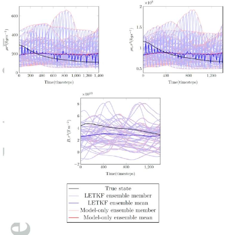
To demonstrate the effectiveness and potential of the LETKF in assimilating solar wind observations, the density, radial momentum and radial magnetic field are plotted at the observation location in Figure 3. Figure 3 shows the model-only ensemble and its mean, in red shades, and the LETKF analysis ensemble, in blue shades, compared to the truth in black, at the observation point, for each variable observed. It can be seen from figure 3 that, for the majority of timesteps, the LETKF analysis state performs much better, for the density and radial momentum variables, at the observation location than the model-only ensemble when an observation is processed by the data assimilation scheme. At each observation timestep, it can be seen that the LETKF trajectory is pulled towards the true state from the model-only ensemble. This results in reduced absolute errors in the LETKF ensemble when compared to the model-only ensemble. However, this improvement in the LETKF is quickly advected away from the observation location, as can be seen both in the ensemble mean but also in each ensemble member. This is to be expected as the model-only ensemble immediately replaces the updated ensemble in the time steps after assimilation due to the strong radial flow. Here, one of the major differences with atmospheric weather data-assimilation can be seen.
Observations of the radial magnetic field component are not currently used in the as-similation, to avoid violation of the∇ ·B= 0 condition. This is the reason why the pure
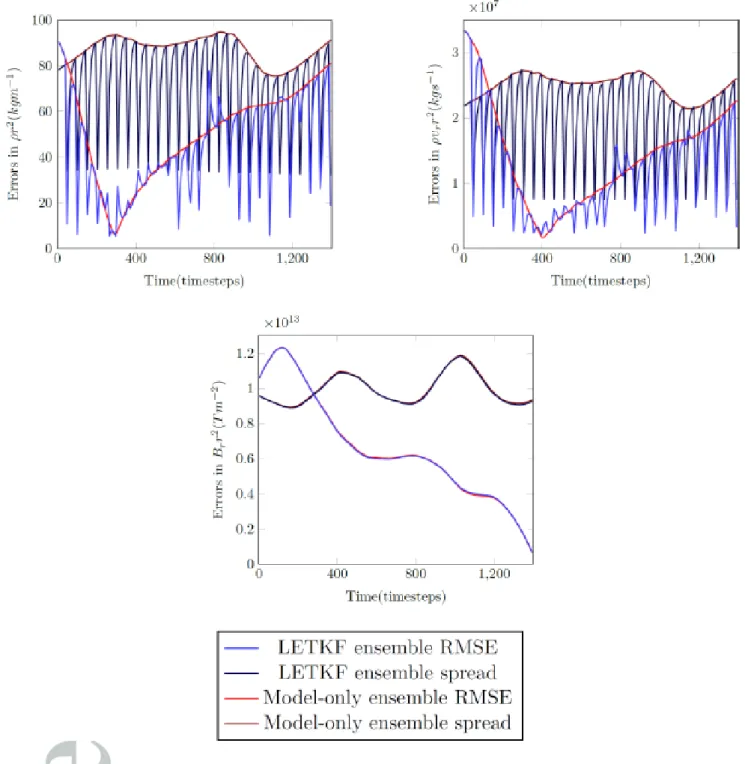
Figure 4 shows the absolute error and ensemble spread for the pure and LETKF ensem-bles. The absolute errors for the pure and LETKF ensemble are shown by the blue and red lines, and the pure and LETKF ensemble spread is shown in dark blue and dark red, respectively. It is encouraging to see that the absolute error and the ensemble spread are of the same order of magnitude, showing that the ensemble is able to represent the uncer-tainty in the estimates well. The absolute error is more variable, but that is to be expected as it is a single realisation of an error, while the ensemble spread is a statistical estimate. The nature of the assimilation updates on the spread and absolute error is consistent with the behaviour of the ensemble members shown in figure 3. Again, due to the strong solar wind any model state update is advected away quickly from this gridpoint, leading to the strong variations in absolute error and spread. The LETKF ensemble spread is reduced to approximately the same value at each analysis timestep, and so does the absolute error, although less consistently. This is to be expected as the prior and the observation error variances have similar value just before each update step.
Figure 4 shows interesting behaviour of the LETKF at some time instances when the absolute error becomes larger at an assimilation step. This is consistent with the behaviour of the ensemble mean in figure 3. The ensemble spread is always decreasing. The latter is consistent with what a Kalman-filter like update should do, the posterior covariance is always smaller than the prior covariance. For the RMSE we have to realise three things. Firstly, it is a random realisation of the error, so it can go up. Secondly, and perhaps more importantly, the updates are not univariate, but all variables are updated at the same time. It is well possible that a smaller RMSE for one variable is compensated by a larger absolute error in another, so that the total variance (defined e.g. as the trace of the
posterior absolute error matrix) is still decreasing. However, this is not what we expect given that we observe all variables at the same time. Thirdly, it might be related to the fact that we do not update the magnetic field. This leads to slightly inconsistent updates, pushing the system out of balance. The model will react by an adjustment process that is typically wavelike. This will not be visible well at the observation location due to the strong solar wind, but might be visible downwind. This seems to be the case, as discussed later.
Figure 5 shows the evolution of the difference of the absolute errors over the spatial domain, as calculated through equation (11). Red areas indicate that the LETKF has reduced the absolute error, while blue areas mean the opposite. The left column shows the density, the middle column the radial momentum, and the last column the radial magnetic field. The rows denote time instances 260 timesteps apart, starting from 60 timesteps into the assimilation run. This frequency is chosen to show the quality of the forecast produced by the LETKF ensemble 10, 20, . . . timesteps after the observation. All fields show positive impact of the LETKF, being advected towards Earth with the solar wind. In the density and radial momentum fields, we see a wavelike update instead of the expected steady update. It is clear that the model is adjusting itself from the assimilation updates by producing a wavelike feature which partly negates the positive impact of the assimilation. The impact on the radial magnetic field seems to be steady until a feature appears after about 1100 time steps.
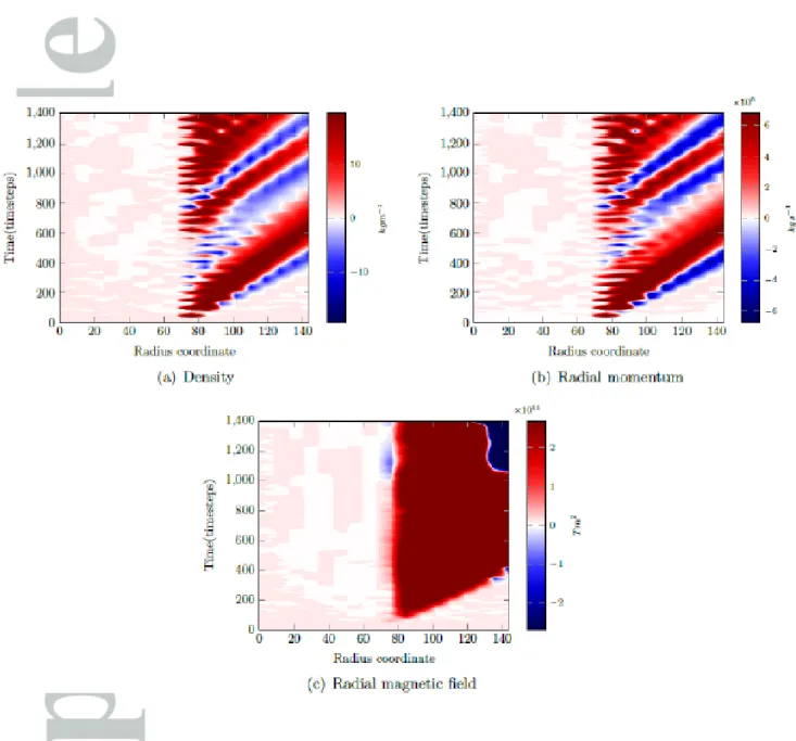
To investigate this further we produce Hovmoller plots along the radial direction for the three variables in figure 6. These confirm the wavelike disturbance in the density and radial momentum fields. The waves are not completely regular but have an average
period of about 500 time steps, corresponding to 1.85 days, with a wavelength of about 60 grid points, which corresponds to 0.45AU. These features are likely to be the result of increased total pressure (the plasma density is increased without a compensating decrease in the magnetic field). Interestingly, this is equivalent to the current method for simulating CMEs within ENLIL, i.e. the insertion of an over-pressured density perturbation at the inner boundary.
7. Data assimilation challenges for space weather models
A major challenge facing the implementation of variational methods in space weather models is the requirement for a tangent linear and adjoint version of the full nonlinear model. The adjoint is an extremely useful tool once developed [Errico, 1997], however, it requires many man-years to code and test, especially for complex models like ENLIL. For less complex MHD models however, it may be possible to code an adjoint for use in solar wind forecasting. One of the main advantages of ensemble-based methods is their ease of implementation on a new problem.
Additionally, variational methods require that a background error covariance matrix is provided for each assimilation window. In other words, the uncertainty regarding the initial condition supplied for use in the data assimilation scheme. This matrix is generated by computing the errors of decades worth of forecasts and reanalysis data, something that is not available to us in the space weather field. For sequentially based methods like the ensemble Kalman filters, this matrix only has to be provided at the start of the data-assimilation effort, but is propagated by the ensemble from then on.
prediction a typical window length is 6 to 12 hours, and it is unclear how long the window can be for space weather applications. It will depend on the spatial resolution of the model, as higher resolution typically means stronger nonlinearities with shorter growth time scales, but also on how close we are to the true solution, so how wide the covariances are. Numerical weather prediction at the global scale is quite accurate due to the enormous amount of relatively accurate observations in each 6 hour window, presently close to 107 observations. This means that the initial guess over the assimilation will be quite accurate too, so that although the full system is very nonlinear, we are so close to the true solution that linearisations work well. Space weather seems to be a long way away from this situation. (This doesn’t mean that variational methods should be abandoned at this stage as one can run an ensemble of variational methods to explore the posterior pdf, similar to an ensemble smoother. This is a technique also used in weather prediction.)
Ensemble Kalman filters such as the one explored in this paper do rely on a Gaussian assumption of the prior pdf, and on the likelihood. These will be violated, but, interest-ingly enough, ensemble Kalman filters have been found to be quite robust to non-Gaussian situations. Although not completely understood, this might be related to the fact that another way to derive the Kalman filter, and to some extent the ensemble Kalman Filters, is to assume that the best estimate is a linear combination of the prior best estimate and the observations. That is often true to first order.
Ensemble Kalman Filters need localisation. The localisation scheme used in these ex-periments was a relatively simple asymmetric distance-based localisation on theRmatrix with a localisation radius of 0.01AU. This localisation radius may not be an accurate length-scale and different variables may require different localisation radii (i.e. spurious
correlations may need to be removed between radial momentum and longitudinal mag-netic field, for example). Additionally, this distance-based localisation scheme is perhaps not ideal for the solar wind simulations, as the variables are highly correlated along the magnetic field lines, but weakly correlated perpendicular to them, due to the ”freezing in” of the plasma and magnetic field. Therefore, an anisotropic localisation scheme that follows the magnetic field lines in the domain may be more realistic and allow for bet-ter assimilation of the observations. Albet-ternatively, if the magnetic field lines cannot be accurately ascertained from the model, then an anisotropic localisation scheme may be more suitable that follows an Archimedean spiral radially outwards from the Sun in the steady flow. When a CME is present the localisation area should probably be closer to an expanding arc. More research is required to adequately analyse appropriate localisation methods for the solar wind.
The magnetic field has the strong physical constraint, ∇ ·B = 0, which needs to be conserved by the data assimilation analysis. For ENLIL, this is difficult to enforce at run time as the model solves for unipolar magnetic field, to minimise numerical diffusion effects. In ENLIL,∇·B = 0 is assumed at the previous timestep and then evolved forward in time such that ∇ ·B remains zero at the next timestep. However, if ∇ ·B 6= 0 at the previous timestep, as a result of the data assimilation breaking the balance present in the system, then ENLIL will not enforce∇ ·B= 0. This will introduce numerical instabilities that may cause the model to become unstable and/or unphysical at future timesteps. This has been verified by experiments performed in Lang (2016) [Lang, 2016].
To get around this issue the B field is removed from the state vector such that the magnetic field is not updated by the data assimilation scheme. This can be used even
when using observations of the magnetic field because the LETKF will use the ensemble-based correlations between the magnetic field and the other state variables to update those. Information of the magnetic field is then passed on from the updated variables to the magnetic field itself through the ENLIL model evolution, in a manner similar to how CMEs are introduced into the ENLIL model. For a MHD code that enforces ∇ ·B = 0 at each timestep (e.g., by solving for the vector potential of the magnetic field), the data-assimilation does not have to ensure that condition, but we can call the model routine to enforce it immediately after the data-assimilation step.
Another area that needs attention is the large range of the variable values between a quiet phase and when a CME is present. When the observations suddenly indicate that a CME is present, a huge change to the model state is enforced by the data assimilation. This change can easily push the model out of balance, resulting in numerical instabilities and potential model instability. Similar problems are encountered in weather prediction, for instance when clouds are detected in observations, but the model doesn’t have clouds at those gridpoints. A cloud represents a completely different themodynamic state of the system, so a large change in several model variables, and this is still an outstanding problem in numerical weather prediction. A potential solution is to use a smoother, so a method that updates the present state using observations from the future, allowing for a smoother transition. A difficulty is space weather is that the sparsity of observations might preclude this solution.
In the experiments performed in Lang (2016) [Lang, 2016], all ensemble members tended to collapse on one model evolution, and the LETKF became ineffective. This was due to the use of the same boundary conditions at the inner boundary, forcing the model
evolutions to become similar quickly due to the highly driven nature of the solar wind. This was especially problematic when a CME was detected in the observations as none of the ensemble members contained a CME. This means that it is vital that different time varying boundary conditions are used in order for ensemble-based methods to work. Again much work is needed to gain experience in what the best way is to solve this problem. Each of these varying boundary conditions has to be a potential realistic realisation of the real boundary condition, which suggests, for instance, that at least a few ensemble members should have a CME at the inner boundary at varying degrees of maturity.
This initial study has assumed that there is no model error present in the ENLIL model, which is obviously a poor assumption. These model errors typically fall under two main categories: systematic model errors and stochastic model error. Systematic model errors can be comprised of errors in the model and biases that are constant over the assimilation window. Any known biases/systematic errors present in the prior model should be removed before the data assimilation is performed, and if they are not known but assumed to be present, they should be estimated. One possible method of diagnosing and removing functional model errors was proposed by [Lang et al., 2016], which use differences between a data assimilation run and a pure model run as a proxy for the model error present. Several methods have been proposed to estimate model biases, such as [Dee, 2005] and [Tremolet, 2006] amongst many others. To incorporate stochastic model uncertainty, it is necessary to generate a stochastic model error covariance matrix, Q, that contains the relevant MHD balances to perturb the ensemble with a model error term at every time step and improve the quality of the assimilation. It is unclear what this matrix should look like, but it is important to realise that it should not contain
the statistics of the missing physics per se, but its influence on the resolved scales. One possible method of doing this would be to start from an initial guess and learn from the data-assimilation experiments what the best formulation is, perhaps exploring techniques from machine learning. The first guess might come from a scaled down version, both in length scale and in amplitude, of a covariance matrix generated from samples of a long model run.
8. Conclusions
This is the first study to incorporate advanced data assimilation methods into solar wind models, building upon the work started in Lang (2016) [Lang, 2016], and these experiments show that the LETKF is a useful tool that has potential for estimating the solar wind. It can be seen that the LETKF can improve upon the model-only ensemble at the observation point and those improvements are advected radially outwards. However, due to the solar wind being a highly-driven system dominated by the dynamics of the Sun, the improvements made by the LETKF at the observation are confined to the magnetic flux tube on which the observation is located.
The density and radial momentum variables were very responsive at the observation point to the data assimilation analysis, moving close to the truth and returning to the background state as this improvement is advected away. However, the sharp gradient caused by this improvement is causing numerical wave-like patterns to form. Further research is required to determine the most effective solution.
The magnetic field vector, however, is not very responsive and does not appear to respond to the changes in the density, temperature and momentum variables. Whilst
(especially in the latitudinal and longitudinal directions, not shown here), it is not be possible to directly assimilate magnetic field observations while enforcing the ∇ ·B = 0 criterion, either by one of the two methods suggested Appendix B, or by rigorously enforcing∇ ·B = 0 at each timestep in the numerical model.
Whilst there are many challenges that still need to be overcome in solar wind data assimilation, these experiments show that data assimilation has great potential for the improvement of solar wind forecasting.
Appendix
Appendix A: Local Ensemble Transform Kalman Filter
The Local Ensemble Transform Kalman Filter (LETKF) was developed by [Hunt et al., 2007], based upon the Local Ensemble Kalman Filter (LEKF) developed by [Ott et al., 2004]. In the LETKF observation localisation is performed. The principle behind the LETKF is to perform the analysis at the grid-points in parallel, updating the state at each grid-point using only observations contained within a local region of that grid-point. The LETKF is an extension of the Ensemble Transform Kalman Filter (ETKF) [Bishop et al., 2001; Majumdar et al., 2002], that transforms the EnKF algorithm into the (typically) lower dimensional ensemble space, allowing more efficient computations.
The LETKF transforms the problem in state space to ensemble space as follows. At each observation time a perturbation matrix is generated for the state, which is defined as:
X= x(1)−x, . . . ,x(M)−x (A1)
and in addition to this, an ensemble of model observations is generated, such that:
Y = y(1)−y, . . . ,y(M)−y. (A2) wherey(m)=H x(m) and y= M1 PM m=1 Hk(x(m)) .
In the LETKF, localisation is performed on the observation error covariance matrix, R, therefore limiting the observations that affect the state in the analysis. This is done by applying a ‘forgetting factor’ [Nerger et al., 2012], υ, to R for each observation, such that the observations further away from the analysis gridpoint get less weight than those
Gaussian function between the analysis gridpoint and the observation gridpoint. The localised observation error covariance matrix shall be denoted byR, where˜
˜ R= 1
υR. (A3)
A matrix C∈RM×Ny is defined such that:
C=YTR˜−1 (A4)
which is used to calculate the matrix, T∈RM×M:
T= M −1 1 +ρ I+CY −1 (A5)
where ρ > 0 is the multiplicative covariance inflation factor. Typical values range from 0.01, up to 10 in extreme cases.
The weighting matrix W ∈ RM×M and mean weighting vector w∈
RM are computed as:
w=TC(y−y) (A6) W= ((M −1)T)12 . (A7)
An ensemble of weight vectors Wa(M) is created by adding wa to the columns of Wa, such that the weight vector for the mth ensemble member is given by:
wa(m) =w+Wm (A8)
whereWm is the mth column ofW.
Then the mth analysis ensemble member is given by:
In this appendix several methods are presented and discussed that enforce∇ ·B = 0 in each updated ensemble member.
1. Enforce ∇ ·B = 0 after the LETKF analysis via a projection method.
Via the Helmholtz decomposition [Arfken et al., 2011], any field can be written as the sum of the curl of another field A and the gradient of a scalar field,ϕ. Therefore, B can be written as:
B =∇ ×A+∇ϕ (B1) Taking the divergence of equation (B1), it can be seen that:
∇ ·B=∇ · ∇ϕ=∇2ϕ (B2)
This is non-zero if ∇ϕ is nonzero. Therefore, in order to preserve the ∇ ·B condition, ∇ϕ, must be subtracted from the DA analysis of the magnetic field variables.
To do this, it is necessary to calculate ∇ ·B and then solve the Poisson equation
∇2ϕ=∇ ·B (B3)
for ϕ.
The issue with this is that the Poisson equation is an elliptic equation that typically has to be solved iteratively, which can be expensive to compute for high-dimensional systems.
2. Encode ∇ ·B= 0 into the Kalman filter update equations via the covariances. For the second method, we starts by looking at the ETKF update equation for the mag-netic field component of the state vector, which is given by:
Ba(M)i =Bfi(M)+ N X m=1 h Bfi(m)−Bfi(M)WiB(m)i (B4)
where Bfi(M) and Ba(M)i are the forecast and analysis magnetic field ensemble, each with
M ensemble members, at timestep i; and WiB(m) are the weights generated, for the mth
ensemble member of the magnetic field variable, by the ETKF methodology. By taking the divergence of the analysis state, we obtain the following equation:
∇ ·Ba(M)i =∇ ·Bfi(M)+ M X m=1 h ∇ ·Bfi(m)− ∇ ·Bf(M)WB(m) i i = 0. (B5)
Using∇ ·Bfi(m) = 0 for each ensemble member from the prior model, and that the prior mean is also divergence-free because the mean is a linear operator, implying∇·Bf(M) = 0, it can be seen that∇·Ba(M)i = 0 for the ETKF. Therefore, the ETKF satisfies the balance equation, as required.
Unfortunately, when we localise the ETKF for the LETKF,WiB(m)will become dependent upon the space domain and hence the divergence of a term within the sum of equation (B4) becomes: ∇ ·Bfi(m)−Bif(m)WiB(m)=∇ ·Bfi(m)− ∇ ·Bif(m)WiB(m) + Bfi(m)−Bfi(M) ∇ ·WiB(m) (B6) which implies ∇ ·Ba(M)i = M X m=1 Bfi(m)−Bfi(M)∇ ·WiB(m) (B7)
To ensure that this equation is equal to zero, it is required that ∇ ·WiB(m) = 0 for all ensemble members. This is of similar complexity to solving∇ ·Ba(m)i = 0 directly for each ensemble member, so it appears little has been gained from this.
3. Solve a variational problem for each ensemble member.
condition can be enforced via a Lagrange multiplier in that variational problem. We will not elaborate on that solution here.
Acknowledgments. The data used are listed in the references, tables and figure cap-tions. The boundary condition data used to initialise the runs is generated from WSA model runs and was provided to us by the Met Office, however, t his data can also be freely downloaded from the repositories athttps://www.ngdc.noaa.gov/enlil/ [2017]. This work was funded by the Natural Environment Research Council under NE/J005878/1. In addition, PJvL thanks the European Research Council (ERC) for funding the CUNDA project under the European Unions Horizon 2020 research and innovation programme.
References
Amezcua, J., M. Goodliff, and P. J. van Leeuwen (2017), A weak constraint 4densemble-var. part i: formulation and simple model experiments, Tellus A, 69.
Anderson, J. (2007), Exploring the need for localization in ensemble data assimilation using a hierarchical ensemble filter,Physica D: Nonlinear Phenomena,230(1), 99–111. Anderson, J., T. Hoar, K. Raeder, H. Liu, N. Collins, R. Torn, and A. Avellano (2009), The data assimilation research testbed: A community facility,Bulletin of the American Meteorological Society, 90(9), 1283.
Archer: http://www.archer.ac.uk/ (2017).
Arfken, G., H. Weber, and F. Harris (2011), Mathematical methods for physicists: A comprehensive guide, Academic press.
Arge, C., and V. Pizzo (2000), Improvement in the prediction of solar wind conditions using near-real time solar magnetic field updates, Journal of Geophysical Research:
Space Physics,105(A5), 10,465–10,479.
Bishop, C., B. Etherton, and S. Majumdar (2001), Adaptive sampling with the ensemble transform Kalman filter. Part I: Theoretical aspects, Monthly Weather Review,129(3), 420–436.
Board, S. S. (2008),Severe Space Weather Events–Understanding Societal and Economic Impacts:: A Workshop Report, National Academies Press.
Browne, P., and S. Wilson (2015), A simple method for integrating a complex model into an ensemble data assimilation system using mpi, Environmental Modelling & Software,
68, 122–128.
Burt, J., and B. Smith (2012), Deep space climate observatory: The DSCOVR mission, inAerospace Conference, 2012 IEEE, pp. 1–13, IEEE.
Cannon, P., M. Angling, L. Barclay, C. Curry, C. Dyer, R. Edwards, G. Greene, M. Hap-good, R. Horne, D. Jackson, et al. (2013),Extreme space weather: impacts on engineered systems and infrastructure, Royal Academy of Engineering.
Cranmer, S. (2008), On competing models of coronal heating and solar wind acceleration: The debate in ’08, arXiv preprint arXiv:0804.3058.
Davis, C., J. Davies, M. Lockwood, A. Rouillard, C. Eyles, and R. Harrison (2009), Stereo-scopic imaging of an earth-impacting solar coronal mass ejection: A major milestone for the stereo mission,Geophysical Research Letters,36(8).
De Moortel, I., and P. Browning (2015), Recent advances in coronal heating,
https://www.ncbi.nlm.nih.gov/pmc/articles/PMC4410557/.
D.P. Dee. Bias and data assimilation. Quarterly Journal of the Royal Meteorological Society, 131(613):3323–3343, 2005.
Errico, R. (1997), What is an adjoint model?, Bulletin of the American Meteorological Society,78(11), 2577–2591.
Evensen, G., D. Dee, and J. Schr¨oter (1998), Parameter estimation in dynamical models, inOcean Modeling and Parameterization, pp. 373–398, Springer.
Eyles, C., R. Harrison, C. Davis, N. Waltham, B. Shaughnessy, H. Mapson-Menard, D. Bewsher, S. Crothers, J. Davies, G. Simnett, et al. (2009), The heliospheric imagers onboard the stereo mission, Solar Physics, 254(2), 387–445.
Fairbarn, D., S. Pring, A. Lorenc, and I. Roulsone (2014), A comparison of 4dvar with ensemble data assimilation methods, Q. J. Roy. Meteorol. Soc., 140, 281–294.
Gloeckler, G., H. Balsiger, A. B¨urgi, P. Bochsler, L. Fisk, A. Galvin, J. Geiss, F. Gliem, D. Hamilton, and T. Holzer (1995), The solar wind and suprathermal ion composition investigation on the wind spacecraft, Space Science Reviews, 71(1-4), 79–124.
Goodliff, M., J. Amezcua, and P. J. van Leeuwen (2017), A weak constraint 4densemble-var. part ii: experiments with larger models, Tellus A, 69.
Gosling, J. T. (1993), The solar flare myth, Journal of Geophysical Research: Space Physics, 98(A11), 18,937–18,949, doi:10.1029/93JA01896.
Gropp, W., E. Lusk, N. Doss, and A. Skjellum (1996), A high-performance, portable im-plementation of the mpi message passing interface standard, Parallel computing,22(6), 789–828.
Hassler, D., I. Dammasch, P. Lemaire, P. Brekke, W. Curdt, H. Mason, J. Vial, and K. Wilhelm (1999), Solar wind outflow and the chromospheric magnetic network, Sci-ence, 283(5403), 810–813.
Hodyss, D., and N. K. Nichols (2015), The error of representation: basic understanding,
Tellus A.
Houtekamer, P., and H. Mitchell (2001), A sequential ensemble kalman filter for atmo-spheric data assimilation, Monthly Weather Review, 129(1), 123–137.
Hunt, B., E. Kostelich, and I. Szunyogh (2007), Efficient data assimilation for spatiotem-poral chaos: A local ensemble transform kalman filter, Physica D: Nonlinear Phenom-ena, 230(1), 112–126.
Jackson, B. (1985a), Helios observations of the earthward-directed mass ejection of 27 november, 1979, Solar physics, 95(2), 363–370.
Jackson, B. (1985b), Imaging of coronal mass ejections by the helios spacecraft, Solar physics, 100(1-2), 563–574.
Kaiser, M., T. Kucera, J. Davila, O. S. Cyr, M. Guhathakurta, and E. Christian (2008), The stereo mission: An introduction, in The STEREO Mission, pp. 5–16, Springer. Kalman, R., and R. Bucy (1961), New results in linear filtering and prediction theory,
Journal of Fluids Engineering, 83(1), 95–108.
Kalman, R. E. (1960), A New Approach to Linear Filtering and Prediction Problems,
Transactions of the ASME–Journal of Basic Engineering, 82(Series D), 35–45.
Kivelson, M., and C. Russell (1995), Introduction to space physics, Cambridge university press.
Lang, M. (2016), Model improvement using data assimilation, Ph.D. thesis, University of Reading.
M. Lang, P.J. van Leeuwen, and P.A. Browne. A systematic method of parameterisation estimation using data assimilation. Tellus A, 68(0), 2016.
Leslie, J., and S. Cole (2016), http://www.nesdis.noaa.gov/dscovr/.
Lopez, R. (1987), Solar cycle invariance in solar wind proton temperature relationships,
Journal of Geophysical Research,92(A10), 11,189–11,194.
Majumdar, S., C. Bishop, B. Etherton, and Z. Toth (2002), Adaptive sampling with the ensemble transform Kalman filter. Part II: Field program implementation, Monthly Weather Review, 130(5), 1356–1369.
Manoharan, P., and S. Ananthakrishnan (1990), Determination of solar-wind velocities using single-station measurements of interplanetary scintillation,Monthly Notices of the Royal Astronomical Society, 244, 691–695.
McComas, D. J., M. Velli, W. S. Lewis, L. W. Acton, M. Balat-Pichelin, V. Bothmer, R. B. Dirling, W. C. Feldman, G. Gloeckler, S. R. Habbal, D. M. Hassler, I. Mann, W. H. Matthaeus, R. L. McNutt, R. A. Mewaldt, N. Murphy, L. Ofman, E. C. Sittler, C. W. Smith, and T. H. Zurbuchen (2007), Understanding coronal heating and solar wind acceleration: Case for in situ near-sun measurements, Reviews of Geophysics,
45(1), doi:10.1029/2006RG000195.
T. Miyoshi, Y. Sato, and T. Kadowaki. Ensemble Kalman Filter and 4D-var intercom-parison with the Japanese operational global analysis and prediction system. Monthly Weather Review, 138(7):2846–2866, 2010.
Nakamura, G., and R. Potthast (2015), Inverse Modeling, 2053-2563, IOP Publishing, doi:10.1088/978-0-7503-1218-9.
Nerger, L., W. Hiller, and J. Schr¨oter (2005), Pdaf-the parallel data assimilation frame-work: experiences with kalman filtering, inUse of high performance computing in meteo-rology: proceedings of the Eleventh ECMWF Workshop on the Use of High Performance