Detrending Time-Aggregated Data

Detrending Time-Aggregated Data

David Aadland

October 2002

Abstract

This paper examines the combined influences of detrending and time aggregation on the measurement of business cycles. The approximate band-pass filter of Baxter and King (1999) performs relatively well in the sense that it retains the basic shape of disaggregate spectra and cospectra when applied to time aggregated data and is straightforward to apply across sampling intervals. Analysis of known time series processes and actual U.S. macro data, as well as simulation of a standard high-frequency RBC model, confirm the theoretical results.

JEL Codes: C1 and E3.

∗_{To be presented at the 2003 Winter Meetings of the Econometric Society, Washington D.C. The author is}

an assistant professor in the Department of Economics, Utah State University, 3530 Old Main Hill, Logan, UT, 84322-3530, 435-797-2322 (phone), 435-797-2701 (fax), [email protected].

1

Introduction

One of the most challenging and controversial aspects of business-cycle research is attempting to remove secular trends from macro data, and do so in a manner that allows one to disentangle the

cyclical and growth components. Much of the controversy stems from the fact that seemingly

innocuous data transformations have been shown to frequently induce undesirable behavior in the residual series. Kuznets’ work in the 1960’s is a classic example of how well-intended data trans-formations can lead to spurious results, such as his discovery of 20-year long swings in economic activity (Adelman (1965); Howrey (1968)). A second example comes from Nelson and Kang (1981), who show that the residuals from a regression of a random walk on time display spurious periodic-ity. The upside of these and other related studies is that practioneers are now more aware of the

possible pitfalls of detrending data. The downside is that, in the process of searching for better

detrending procedures, the number of alternative detrending methods have grown rapidly. On

the surface, it would seem that having more detrending options available would be advantageous, but unfortunately these procedures often produce widely varying pictures of the business-cycle and economic theory is rarely sharp enough to make recommendations about which method is

appro-priate (Canova (1998)). Therefore, empirical macroeconomists are often left to choose from the

various detrending options with little guidance. This paper attempts to shed further light on which detrending methods are most desirable by examining their ability to detrend temporally aggregated

data without distorting the underlying behavioral properties of the economic series. This is an

important criterion because nearly all macroeconomic data are heavily aggregated over time. The focus is on three of the most commonly used detrending methods in empirical macroeconomics: the

first difference (FD), the Hodrick-Prescott (HP), and the Baxter-King (BK) approximate band-pass

filters.

Over the last two decades, the FD filter has been a popular method for removing the trend

from nonstationary time series. This is due in large part to Nelson and Plosser (1982), who argue

that many macroeconomic time series are difference, rather than trend stationary. When a series

is measured in natural logarithms, the resulting FD-filtered series are approximate growth rates

problem, however, with treating growth rates of series as business-cycle fluctuations is that the

FD filter tends to exacerbate high-frequency noise and introduce a phase shift. Despite these

criticisms, many prominent studies of business-cycle phenomena continue to examine the growth rates of macro series (e.g., Campbell (1999), Cogley and Nason (1995a), and Plosser (1989)). An advantage of the HPfilter, relative to the FD filter, is that it does not exacerbate high-frequency noise and does not introduce a phase shift into the data. As a consequence, the HPfilter, introduced by Hodrick and Prescott (1980), has arguably become the “industry standard” for detrending data

in empirical macroeconomics. This flexible detrending method trades off deviations from trend

against an adjustable smoothness criterion. The HP filter, however, is not without its critics. It

has been criticized for generating spurious cycles in difference stationary data (Harvey and Jaeger

(1993); Cogley and Nason (1995b)); altering the persistence, variability and co-movement of time

series (King and Rebelo (1993)); and (similar to the FDfilter) for passing through high-frequency

or “irregular” variation. The third detrending method I consider is the BKfilter. This procedure,

introduced by Baxter and King (1999), is based on the well-established concept of a spectral

band-pass filter. A primary advantage of the BK filter is that it is more consistent with the Burns

and Mitchell (1946) definition of the business cycle as containing cycles that last between six and

32 quarters. Although relatively new, the BK filter appears to be gaining in popularity and has

recently been employed by studies such as Basu and Taylor (1999) and by Stock and Watson (1999)

in theHandbook of Macroeconomics to document various business-cycle facts.

In addition to filtering out a trend, most macro time series are also implicitly passed through

a time-aggregation (TA) filter. For institutional reasons, business-cycle researchers work almost

exclusively with quarterly data. Since data-generating processes for economic data are generally thought to operate at continuous or very short discrete-time intervals, observed quarterly data

are therefore some sort of transformation of the high-frequency data. If the variable is a flow,

then it is typically summed (or averaged) over shorter time intervals. If it is a stock, then it is

typically systematically sampled. Ideally, we would like time aggregation to preserve as many of

the underlying properties of the high-frequency data-generating process as possible. This and

other aspects of time aggregation have been extensively explored both in the time domain (e.g., Tiao (1972); Weiss (1984); and Rossana and Seater (1992)) and in the frequency domain (e.g., Sims

(1971) and Granger and Siklos (1995)).

The unique contribution of this paper is to examine how the joint application of detrending

and TA filters influence how we look at business cycles. As mentioned above, there are many

studies that examine the individual effects of detrending and time aggregation, but despite the fact

that detrending and time aggregation are almost always joint phenomena, few have examined their

combined effects. The results in this paper suggest that the interaction between the twofilters is

important for how we measure business cycles and test our models. The criteria used in this paper to contrast the various detrending filters is (1) their ability to maintain the spectral properties of time series generated by economic decisions at shorter, more frequent intervals and (2) their ease of use across frequencies. Recent research (e.g., Heaton (1993), Chari, Kehoe and McGratten (2000), and Aadland (2001)) has shown that temporal aggregation of data generated at higher frequencies

can have important effects on the behavior of economic time series and evaluation of various models.

The argument is not that we need to employ or collect data at more frequent intervals, as that may introduce unnecessary measurement error, but rather that we need to explicitly model that sampling and aggregation process that is implicit in almost all macro data. This can be done by solving and calibrating macroeconomic models at higher frequencies and aggregating them up to the data-sampling interval. The primary concern in this paper is how does the time aggregation that is implicit in the actual data and explicit in the artificial data of high-frequency theoretical economies interact with the detrending process? And can the results from this exercise be used to support some detrending methods over others?

The remainder of the paper is as follows. Section 2 introduces the various detrending and TA filters and discusses their cascading. Section 3 investigates the practical ramifications of jointly

applying thesefilters through experiments with known time-series processes and actual macro data.

Section 4 applies the analysis to a temporally aggregated, high-frequency RBC model. Section 5 concludes.

2

Temporal Aggregation and Detrending Filters

The most transparent method for investigating the effects of detrending and TAfilters is through

spectral analysis. A brief review of spectral analysis as it relates to filtering theory is included in Appendix A. For a more thorough coverage of spectral analysis and its applications see Priestley

(1988) or Hamilton (1994). In this section, I focus on the properties of the TA and detrending

filters individually, as well as their combined or “cascaded” effect.

2.1

Temporal Aggregation Filters

I use the term temporal aggregation to refer to a mapping of either a continuous or short-interval discrete time series process to a longer-interval discrete time series process. Although this paper focuses exclusively on discrete-time processes, the results could be generalized to handle

underly-ing continuous-time processes (e.g., see Sims (1971), Geweke (1978) or Sargent (1987)).

Time-aggregated flow data are most often either summed or averaged over time while stock data are

typically systematically sampled at regularly spaced discrete-time intervals. Time aggregation,

whether a flow or a stock variable, can be thought of as involving a two-step process (Lippi and

Reichlin (1991)). In step one, the variable is passed through an aggregation filter. For example,

under temporal summing the filter is hT S(L) = 1 +L+L2+...+Ln−1, where n indicates the

number of disaggregate (often referred to asbasic) periods being aggregated; and under systematic

sampling the aggregationfilter ishSS(L) =Lk, wherek∈{0,1, ..., n−1}.1 Step two then involves

systematically sampling every nth _{observation from theh}

T S(L)- orhSS(L)-filtered data to form a

series of non-overlapping aggregates.

In terms of their spectra, a temporally aggregated series can be related to its disaggregated

counterpart using the z and Fourier transforms of h(L) and the folding operator (Sims (1971);

1_{For example, when aggregating a monthlyflow variable to an annual frequency,n= 12. Aggregating a weekly}

flow variable to an annual frequency, givesn = 52. Asn _{→ ∞}, one can think of the underlying data generating process as operating in continuous rather than discrete time.

Granger and Siklos (1995)) which is given by F[sx(ω)] = I X j=−I sx(ω+ 2πj/n) (1)

where F[sx(ω)] is defined over ω ∈(−π/n, π/n]and I is the largest number such that ω+ 2πj/n

falls in the range (₋π, π]. The folding operator reflects the well-known aliasing identification problem, whereby harmonics at various frequencies cannot be distinguished from one another in

sampled data.2 In essence, aliasing dictates that frequencies outside the (₋π/n, π/n] range of

the time-aggregated process get successively folded back into the (₋π/n, π/n]range. The initial

folding point,π/nin this context, is sometimes referred to as the Nyquist frequency. Alternatively,

the basic and time-aggregated series can be related in the time domain according to their ACGFs. These are respectively

gy(z) = ∞ P j=−∞ Γjzj and gY(z) = ∞ P j=−∞ Γnjzj, (2)

where theΓ’s are the autocovariances of thehT S(L)- orhSS(L)-filtered data, and lower- and

upper-case letters (i.e., y and Y) refer to the pre-sampled and post-sampled series. From (2), it is clear

that time aggregation produces an aggregate ACGF which is simply a sampled version of the basic

ACGF at equally spaced n-length intervals.

Returning to the frequency domain, the spectra of a time-aggregated series _{Y_} is then

sY(ω) =F[sy(ω)] =F[f(ω)sx(ω)], (3)

wheref(ω) is the squared gain and sY(ω)is defined over(−π/n,−π/n]. Alternatively, one could

redefine sY(ω) in terms of aggregate time and write it assY(˜ω), whereω˜ = ωn∈(−π, π]. Since

the folding operator F is an operator rather than a linear filter, there does not exist a unique

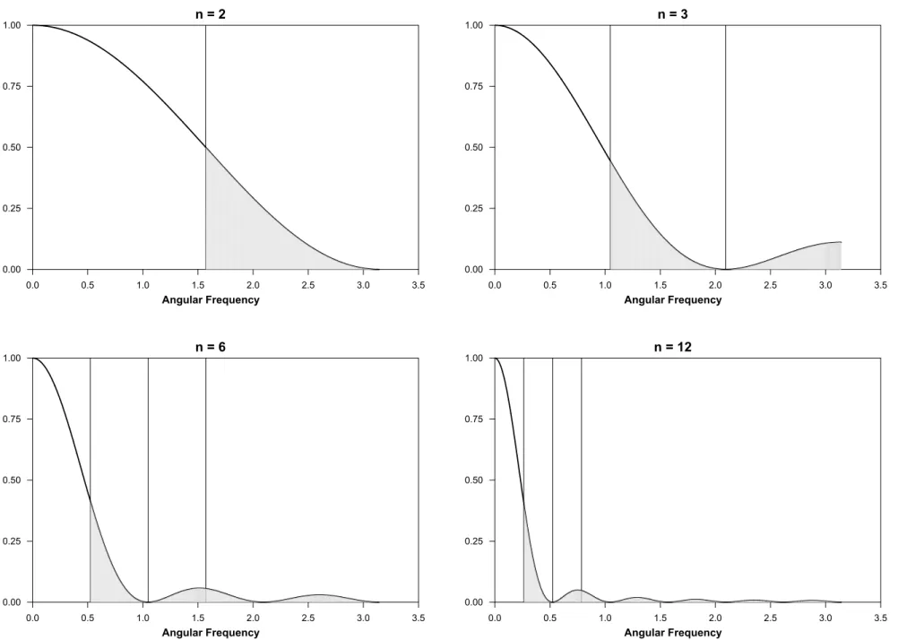
transfer function for time aggregation of any covariance-stationary time series. Figure 1, however,

2_{When sampling from a continuous time process, I is set to}

∞as frequencies larger than π in magnitude are also aliased (Sims (1971)). Since I am treating the underlying process as one set in discrete time, conceptually, one can imagine that frequencies higher than π have been previously aliased in the sampling from an underlying continuous-time process.

shows the squared TA transfer function associated withhT S(L)/n along with the (shaded) aliased

frequencies that will be consecutively folded back (first few folds are shown with vertical lines) onto

the range (0, π/n]. Clearly, the systematic sampling step associated with temporal aggregation

produces a loss of information as some higher-frequency harmonics in the basic series will become

convoluted with lower-frequency harmonics. The extent to which this convolution is important

depends on the nature of the underlying time series, and in particular, on the relative power of

the disaggregate spectrum at cycles with periods greater than 2n basic periods. The practical

importance of this aliasing problem will be explored in more detail below.

These results also extend naturally to a vector time series, with each individual series potentially

filtered in a different manner. In this case the cross spectrum between the time aggregatesY1 and

Y2 is

sY12(ω) =F[sy12(ω)] =F[h1(e−

iω_)h

2(eiω)sx12(ω)]. (4)

2.2

Detrending Filters

As mentioned in the Introduction, there are many different methods that have been applied in

business-cycle research to detrend nonstationary time series. In this paper, I focus on three

de-trending methods — the FD, HP, and BKfilters. The properties of thesefilters are well documented

(e.g., see King and Rebelo (1993) and Canova (1998)), so I will only briefly review their properties.3

First, the FD filter is given by h(L) = 1₋L, which implies that the corresponding squared

transfer function is f(ω) = 2(1₋cos(ω)). Since f(0) = 0, the FD filter removes variation due to

the lowest frequency cycles, but unnecessarily magnifies high-frequency variation as can be seen in

Figure 2. Another undesirable property of the FD filter is that since it is an asymmetricfilter, it introduces a phase shift into the filtered time series.

3_{I do not directly investigate the effects of detrending via regressions of polynomials in time because it is seldom}

used in modern business-cycle research, in part due to Nelson and Plosser (1982) whofind that many macro series are consistent with difference rather than trend-stationary specifications.

Second, the infinite-sample version of the HP filter solves the following problem min {gt} ( _∞ X t=−∞ [yt−gt]2+λ ∞ X t=−∞ [(gt+1−gt)−(gt−gt−1)]2 ) (5)

whereλis an adjustment parameter that governs the growth componentgt by trading offsquared

deviations from trend against a smoothness constraint. King and Rebelo (1993) show that the

filter for the cyclical portion (yt−gt) of thisfilter can be written as

h(L) = λ(1−L)

2₍₁

−L−1)2

1 +λ(1₋L)2_(1−L−1₎2. (6)

Given the four first-difference terms in the numerator of (6), the cyclical portion of the HPfilter

produces a stationary series for any underlying series integrated up to the fourth degree.

Fur-thermore, since (6) is a symmetric filter, it does not introduce any phase shift. When λ= 1600,

the transfer function associated with (6) is an approximate high-pass filter that when applied to

quarterly data approximately removes the variation associated with cycles of period longer than 32

quarters. The HP filter forλ= 1600is shown in Figure 2.

Third, the BK filter of Baxter and King (1999) is an approximate band-pass filter that is

commonly used to eliminate variation associated with cycles of period less than six and more than 32 quarters (i.e., a BP(6,32)filter). The BP(6,32)filter, however, cannot be applied tofinite time series because it involves an infinite number of weights in the linear filter.4 Nevertheless, Baxter

and King (1999) show how to calculate an approximate BP(6,32)filter by minimizing the deviation

of the ideal and actual weights subject to the constraints that (1) the weights are truncated at

K; (2) thefilter does not introduce a phase shift; and (3) the associated transfer function removes

all variation at the zero frequency (i.e., eliminates certain trends). The BK filter (K = 6) that

solves this problem is depicted in Figure 2. The BK filter provides a good approximation to the

ideal BP(6,32) filter with moderate leakage, compression and exacerbation, using the terminology

of Baxter and King (1999). However, the BKfilter involves a trade-off. Higher values ofK, all else

4_{The HPfilter as described above essentially suffers from the same problem since its interpretation as a high-pass}

filter are based on an infinite sample size. Baxter and King (1999) discuss the consequences of applying the HPfilter tofinite samples.

equal, lead to better approximations of the ideal BPfilter, but it require a loss of2K observations.

2.3

Cascading the Time-Aggregation and Detrending Filters

The previous two subsections discussed the individual effects of temporal aggregation and

detrend-ing on a time series. In the context of business-cycle research, however, these twofilters are almost

always applied together. Despite this fact, there have been very few studies that examine their

joint influence. The only papers I am aware of that recognize the dual nature of detrending and

time aggregation are Lippi and Reichlin (1991); Ravn and Uhlig (2002); Baxter and King (1999);

and Maravall and del Rio (2001). Lippi and Reichlin (1991) are primarily concerned with the

sensitivity of trend-cycle variance ratios and measures of persistence to the level of temporal

aggre-gation in the data. The other three papers focus on the relationship between the HPfilter and the

observational frequency of the data. Baxter and King (1999) briefly mention that it is not clear

how to adjust λacross frequencies but suggest that in annual data, λ= 10 appears to work well,

as opposed to the standard values ofλ= 100 orλ= 400. Ravn and Uhlig (2002) provide a more

thorough analytical analysis of howλshould be adjusted across frequencies and suggest, as a rule

of thumb, it should be multiplied byn−4. Finally, a working paper by Maravall and del Rio (2001)

suggest that the HP filter does not preserve itself under temporal aggregation in the sense that

temporally aggregated HP-filtered data cannot be seen as HP-filtered temporally aggregated data.

None of these papers, however, provide a systematic analysis of how the most commonly used

detrending filters preserve the basic properties of temporally aggregated macro data or whether

this criterion can be used to choose amongst the various detrending procedures. To address these issues, one mustfirst examine the joint properties of the detrending and TAfilters, which I turn to now.

Typically macro data are aggregated over time before they are detrended. Accordingly, the

spectrum of the detrended, time-aggregated series can be related to the spectrum of the basic series according to

sY(ω) =fDT(ω)F[fT A(ω)sx(ω)], (7)

aggregation and detrending respectively. Expanding (7) using (1) produces sY(ω) =fDT(ω)fT A(ω)sx(ω) +fDT(ω)fT A(ω) I X j=−I,j6=0 sx(ω+ 2πj/n), (8)

where again I is the largest number such that ω+ 2πj/nfalls in the range (₋π, π]. As (8) shows,

the cascaded transfer function can be decomposed into two parts — thefirst operates on the lower

frequency range ofx(i.e.,ω _∈(₋π/n, π/n]) and the second operates on the higher frequencies that are aliased withω _∈(₋π/n, π/n].

Figure 3 depicts the cascaded (squared) transfer functions associated with time aggregation

(n= 3) and the FD, HP and BKfilters. As in Figure 1, the aliased frequencies are shaded and will

be sequentially folded onto the range ω _∈ (₋π/n, π/n]. It is clear from Figure 3, which presents

the temporal averaging (hT S(L)/n) case, that FD- and HP-filtered time-aggregated data will tend

to suffer from the aliasing identification problem in that they pass through aliased frequencies.

The BK filter, on the other hand, by only passing through cycles with periods between six and

32 quarters, tends to remove the frequencies that suffer the most from the aliasing identification

problem in time-aggregated data. A similar story (figure omitted due to space limitations) emerges

from the systematic-sampling filter, hSS(L) =Lk, where k ∈{0,1, ..., n−1}. Since the squared

transfer function for hSS(L) is always fT A = 1, the cascaded transfer functions associated with

systematic sampling and the three detrending options essentially become an extended (i.e.,ω > π)

version of Figure 2 with thefirst folding point atπ. In general, the aliasing problem is more severe when detrending systematically sampled as opposed to temporally summed (or averaged) data. It is important to note, however, that irrespective of whether the data are temporally summed or

systematically sampled, the BK filter tends to pass through less of the variation associated with

aliased frequencies than the HP filter or especially the FDfilter.

The analysis above extends to the co-movement between two series in a similar manner. The

spectrum of the unfiltered underlying seriesx1 and x2 according to sY12(ω) =f DT 12 (ω)f12T A(ω)sx12(ω) +f DT 12 (ω)f12T A(ω) I X j=−I,j6=0 sx12(ω+ 2πj/n), (9)

wheref₁₂DT(ω) =h1,DT(e−iω)h2,DT(eiω) andf12T A(ω) =h1,T A(e−iω)h2,T A(eiω) are the cross transfer

functions for detrending and time aggregation respectively. Although variables will typically be

detrended in the same fashion, they may be subject to different types of time aggregation. For

example, when considering the co-movement between a stock and aflow variable, one series may be

systematically sampled while the other is temporally summed. In this case, the time aggregation cross transfer function fT A

12 (ω) is likely to involve an imaginary component. Focusing exclusively

on the cospectrum (i.e., real part of the cross spectrum) betweenY1 andY2, we can write

cY12(ω) = Re[f DT 12 (ω)f12T A(ω)]cx12(ω) + Re[f DT 12 (ω)f12T A(ω)] I X j=−I,j₆=0 cx12(ω+ 2πj/n)−   Im[f DT 12 (ω)f12T A(ω)]qx12(ω) + Im[f DT 12 (ω)f12T A(ω)] I X j=−I,j6=0 qx12(ω+ 2πj/n)   (10)

whereRe[z]andIm[z]refer to the real and imaginary parts ofz, respectively. The basic quadrature,

qx12, shows up in the formula for the aggregate cospectra,cY12, because the cascaded cross transfer

functions may involve imaginary numbers, which will in turn be multiplied by the imaginary number

associated with qx12. Figure 4 depicts the real and imaginary parts of the transfer function from

sx12 tocY12 for two detrended, temporally aggregated time series — one temporally averaged using

hT S(L)/nand one systematically sampled usinghSS(L) =L0, where in both cases n= 3. Again,

aliased frequencies are shaded and vertical lines represent folding points. What stands out the

most in Figure 4 is the fact that the FDfilter, and to a lesser extent the HPfilter, behave differently when applied to aggregate data than when applied to basic data. For example, even the non-aliased

portion of the HP filter is no longer an approximate high-pass filter. Furthermore, both the FD

and HPfilters suffer more acutely from the aliasing problem than does the BKfilter, both in terms of the real and imaginary components of the cross transfer functions.

3

Application to Various Time Series Processes

In this section, I examine a set of known time series processes and a set of actual U.S. time series.

Both sets of time series processes are subjected to aggregation and detrending filters to see the

practical importance of jointly applying these twofilters. The advantage of looking at thefirst set of data-generating processes is that the population spectra are known at the high-frequency level. The advantage of looking at actual U.S. time series is that they are likely to be more representative of the actual data used by empirical macroeconomists.

3.1

Known Time Series Processes

I begin by considering four simple time series processes to highlight how time aggregation and

detrending operate together to effect the spectra of a basic series. The four processes are assumed

to take the form

xt = τt+ t (11)

xt = τt+ 0.5xt−1+ t (12)

xt = τt+ t+ 0.5 t−1 (13)

xt = τt+ 0.5xt−1+ t+ 0.5 t−1 (14)

where τt = a+bt is a deterministic linear trend, and t is assumed to be mean-zero, white-noise

process. Since all four series are non-stationary, they do not have a spectral decomposition.

Application of the detrending filters, however, can be thought to work in two steps (Cogley and

Nason (1995b)). In step one, the filter makes the series stationary by linearly detrending, and

then in step two, the filter acts upon the stationary series that remains. The four processes are

aggregated over time using thefilterhT S(L)/nwithn= 4. Conceptually, one can imagine the data

as being generated at quarterly intervals but the researcher only observes time-aggregated annual

observations. Since the BK filter is designed to only pass through cycles with periods between

eight and 1.5 years, it becomes an approximate high-pass filter because cycles with periods of less

annual data is set at λ= 6.25 as suggested by Ravn and Uhlig (2002). Similar annual values for

λare suggested by Baxter and King (1999) (λ= 10) and Maravall and del Rio (2001) (λ= 7).

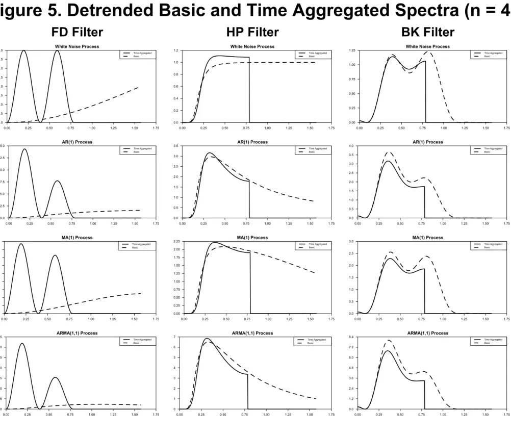
Figure 5 depicts the spectra for detrended, basic _{xt} and detrended, time aggregated {xt}

using the FD, HP and BKfilters. There are several interesting features of the graphs in Figure 5.

First, and most starkly, it is clear that the FDfilter, when applied to time-aggregated data, greatly distorts the spectral representation of the basic series. Since the FDfilter is being applied to

time-aggregated rather than basic data, it takes the formh(L) = 1₋Ln with squared transfer function

f(ω) = 2(1₋cos(nω)). As a result, the FD filter applied to time-aggregated data experiences a

phase shift relative to the basic FD filter that decreases the length of its periods by a factor of

n. Whereas the FDfilter applied to the basic data tends to monotonically magnify high-frequency

variation (see Figure 2), the FDfilter applied to time-aggregated data tends to produce spectra with

multiple peaks. For the case ofn= 4, the peaks are associated with cycles that have periodicity of

approximately 10 and 30 quarters. Consequently, the combined use of time-aggregated data and first-differencing can produce variation at business-cycle frequencies, even when it is absent in the

basic data.5 Second, there is a moderate amount of aliasing present in the HP-filtered spectra,

most of it occurring around theω=π/nfrequency.6 _{Third, at least for time-series processes given}

by (11) - (14), the BK and HP cascadedfilters are surprisingly similar and both act as approximate

high-passfilters when applied to time-aggregated data.

3.2

Actual U.S. Time Series

Next, I examine how time aggregation and detrending influence the spectra of three U.S. macro time

series — GDP, Standard and Poors 500 index (SP500) and consumption. The sources and detailed

definitions of these variables are included in Appendix B. GDP is recorded on a quarterly basis

while SP500 and consumption are recorded on a monthly basis. For the purpose of this exercise, these are treated as the basic timing intervals or high frequencies. Each series is then artificially

aggregated to an annual interval — GDP is temporally summed (n = 4), SP500 is systematically

5_{This result is related to the finding of Working (1960), who showed that a first-differenced, time-aggregated}

random walk contains a moving average term.

6_{To see this most clearly, contrast the HP-TA cascaded (squared) transfer function in Figure 3 with the HP}

sampled in December (n= 12), and consumption is temporally summed (n= 12). Before and after

aggregation, each series is detrended using the three detrendingfilters discussed above. Estimated

spectra are then produced using a modified Bartlett kernel (see Appendix B for more details) for

each of the detrended series at their basic and annual sampling intervals.

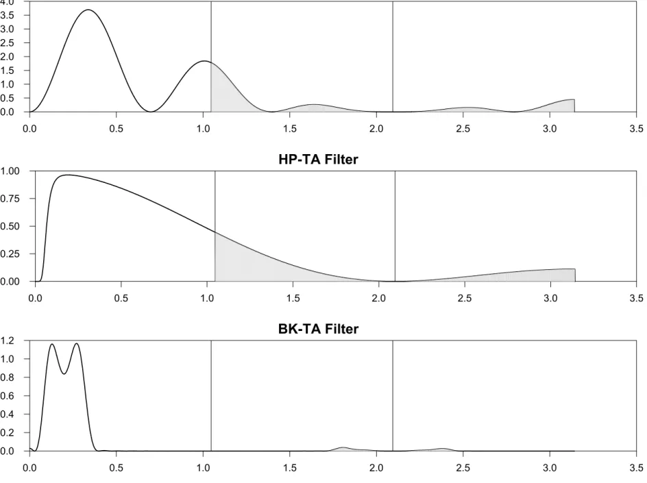
Figures 6a, 6b and 6c depict the estimated spectra for GDP, SP500 and consumption for various detrending methods and frequencies. Beginning with the spectra for GDP in Figure 6a, the three

panels represent FD-, HP- and BK-filtered data with the quarterly angular frequencies measured

along the horizontal axis. The right scale measures the quarterly spectra and the left scale measures

the annual spectra. As in Figure 5, the low-frequency spectra are superimposed over the

high-frequency spectra, with the vertical line representing thefirst fold, or stated differently, the shortest cycles (8quarters= 2π/(ω= 0.785)) that are observable in the annual data. The most important feature of Figure 6a is that (despite the fact that GDP is dominated by lower-frequency cyclical

variation) the estimated spectra for the time-aggregated annual growth rate of GDP in the first

panel clearly distorts the spectral properties of quarterly GDP in terms of their relative magnitudes

and timing of peaks and troughs. The same distortion is not present in the HP- and BK-filtered

data shown in panels two and three where the quarterly and annual lines have nearly identical shapes.

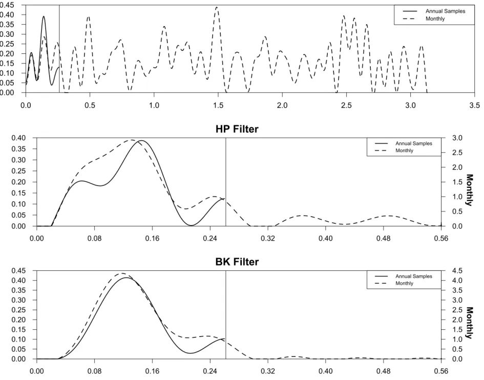
Figures 6b and 6c differ from Figure 6a in that the two basic series are monthly rather than

quarterly so that there is a greater degree of aggregation. In response, I have chosen to show the entireω_∈[0, π]range for only the FDfilter, which displays significant high-frequency variation. In the HP and BKfilter cases, only a small windowω _∈[0, π/6]is shown because there is little-to-no high-frequency variation towards the right-hand-side of the graph. Similar to the GDP case, the

FD-filtered time-aggregated annual data experiences substantial distortion relative to the monthly

spectra. As expected, the distortion due to the aliasing of high-frequency variation is more acute with the systematically sampled SP500 in Figure 6b than with temporally summed consumption in

Figure 6c. The difference between systematic sampling and temporally summing is also highlighted

by contrasting the results using the HP and BK filters. In the case of consumption, which is

temporally summed, the annual estimated spectra are similar whether one uses the HP or BK filter. However, in the case of systematically sampled SP500, the fact that the HPfilter (unlike the

BKfilter) is a high-passfilter and the SP500 contains substantial high-frequency volatility, explains why there is noticeable distortion due to aliasing in the annual HP-filtered data but not the annual

BK-filtered data. Overall, the findings in Section 3 indicate a potential for serious (moderate)

aliasing distortion when using the FD (HP) filter to detrend temporally aggregated data that are

associated with significant amounts of underlying high-frequency volatility.

4

Application to Real-Business-Cycle Theory

In this section, I investigate the practical consequences of detrending time-aggregated data within the context of a simple RBC model, similar to the one presented in King, Plosser and Rebelo (1988). The motivation for this exercise is to build a high-frequency theoretical model that might be thought to more closely represent the actual frequency at which economic agents make decisions. Then a calibrated version of the model is solved and used to generate artificial high-frequency data. The high-frequency data are then temporally aggregated (similar to the manner in which the actual data are aggregated), detrended, and compared to the actual U.S. data at the standard quarterly

frequency. In this manner, it is possible to examine how closely the detrended, time-aggregated

data resemble the underlying properties of the high-frequency data. Similar procedures have been employed by Chari et al. (2000), Aadland (2001), and Cogley and Nason (1995a).

Begin by letting the basic decision interval (assumed to be one week) be indexed by t. A

representative agent is assumed to maximize an expected stream of discounted utility

U(C, L) =Et ∞ X s=0 βt+s · log(Ct+s) + φ ηl η t+s ¸ (15)

by choosing consumption and leisure paths, where Et is the mathematical expectations operator

conditional on all information dated time t and earlier, β a subjective discount factor, Ct

con-sumption, φ leisure’s weight in total utility, lt = (N −Lt)/N the proportion of endowed time

and 1/(1₋η) the intertemporal elasticity of proportional leisure.7 Consumption is subject to the resource constraint

Ct≤Yt−It, (16)

whereYtis output andItgross investment into the capital stockKt. Capital accumulates according

to

It=Kt+1−(1−δ)Kt, (17)

and output is given by the production function

Yt=AtKtα(ztLt)1−α, (18)

where zt/zt−1 = exp(µ) is a deterministic labor-augmenting technology process. Total factor

productivity (TFP) follows the process At = Aρt−1exp( t), where t is a mean-zero, white noise

process with standard deviationσ.

The consumption and labor Euler equations for this problem are

C_t−1 = βEt £ C_t−₊₁1(1 +αYt+1/Kt+1−δ) ¤ (19) (1₋α)Yt/Lt = φltη−1Ct/N. (20)

I turn now to calibrating a weekly version of the RBC model. Since weekly data are generally not available, I use an analog version of the model in quarterly time along with some consistency

conditions for time aggregation that should be satisfied in the steady state. In other words, I

impose that steady-state flow variables in quarterly and weekly time (denoted F and F_∗) should

obeyF =nF_∗, where n= 13. For stocks, the variables should obeyS =S_∗. These constraints are

then substituted into the weekly, steady-state version of the RBC model and solved jointly with

7_{The steady-state intertemporal elasticity of labor is also1/(1}

−η)under the assumption that equal proportions of time are spent in leisure and labor activities.

the corresponding quarterly steady-state equations to get β_∗ = βneµ/n³eµ+β(eµ/nn₋eµ)´−1 (21) δ_∗ = (δ/n) + (1₋eµ/n) + (1/n)(eµ₋1) α_∗ = α η_∗ = η+ log(φ/φ_∗)/log(l) µ_∗ = µ/n,

where asterisks denote weekly parameters.

There are six unknown parameters in (21) and only five equations. To identify the system

I impose an additional restriction that η_∗ be consistent with microeconomic evidence on

high-frequency intertemporal elasticity of substitution in labor. Although the microeconomic evidence

does not pin down an exact value for η_∗, the evidence confirms the expectation that individuals

are more willing to substitute labor across shorter time periods and provides a general guide as to

the appropriate magnitude for η_∗. I specify that the weekly intertemporal labor supply elasticity

is three times as large as its quarterly counterpart, which is roughly in line with microeconomic evidence (e.g., Kimmel and Kniesner (1998), Browning, Hansen and Heckman (1999), Abowd and

Card (1989) and MaCurdy (1983)).8 See Aadland and Huang (2001) for a more detailed discussion

of this calibration procedure and the empirical evidence regarding labor supply elasticities across

data frequencies. Furthermore, steady-state conditions are not helpful in pinning down weekly

values for ρand σ. As in Chari et al. (2000), I specify that the weekly value of ρis equal to its

quarterly value raised to the 1/13th power. The weekly value ofσ is chosen to be consistent with

the standard deviation for the error in a quarterly, time-aggregated version of the TFP process,

which is set at σ = 0.9. Further details regarding the calibration of ρ and σ are outlined in

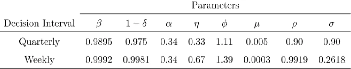
Appendix B. Table 1 depicts commonly chosen quarterly parameter values and the implied weekly parameter values.

8_{The qualitative results with respect to temporal aggregation and detrending are robust to reasonable variations}

Table 1. RBC Parameters Values

Parameters

Decision Interval β 1₋δ α η φ µ ρ σ

Quarterly 0.9895 0.975 0.34 0.33 1.11 0.005 0.90 0.90

Weekly 0.9992 0.9981 0.34 0.67 1.39 0.0003 0.9919 0.2618

The linearized version of the model, coupled with the calibrated parameter values in Table 1,

are then used to simulate 100 artificial time series. Given that the labor-augmenting technology

process (zt) is trend stationary, series such as output, consumption, investment and real wages

will fluctuate about a linear trend. Accordingly, the artificial weekly data are first detrended

and then the resulting series are used to estimate standard deviations, correlations, spectra and cospectra for select series. To investigate the effects of time aggregation, the weekly data are first

temporally aggregated in a manner consistent with the U.S. data-collection procedures. Then

the time-aggregated artificial quarterly data are detrended and used to estimate similar statistics. Lastly, actual detrended quarterly U.S. data are analyzed in a similar fashion. Appendix B provides additional details regarding the US data, detrending procedures, time-aggregation methods, and estimation of the spectra and cospectra.

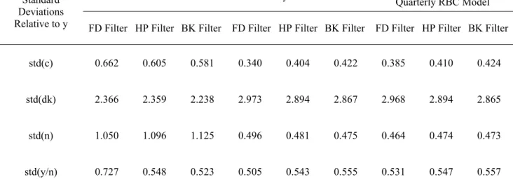
Begin by considering standard deviations and correlations in the time domain, which are shown

in Table 2. The second-moment properties of the simple RBC model are well known (King and

Rebelo (1999)). The model does a good job in predicting the fact that consumption is less volatile than output; that investment is more volatile than output; and that consumption, investment and hours worked are procyclical. However, the simple RBC model tends to produce too little volatility in hours worked and predicts grossly counterfactual positive correlations between average labor

productivity (or equivalently real wages) and hours worked. To examine the effects of detrending

and time aggregation, it is necessary to contrast the results from the weekly and time-aggregated quarterly RBC models. Begin by noticing that the relative volatility predictions are comparable

both across decision intervals and detrending methods, although the differences between the weekly

and quarterly RBC models are somewhat larger underfirst-differencing as compared to either the

Next consider the cross correlations for the weekly and time-aggregated quarterly RBC models.9 The HP and BK cross correlations are quite similar across weekly and quarterly models. Taking this together with the standard deviation evidence suggests that the interaction of time aggregation

and either the HP or BK filters produces limited distortion of the basic second moments (from

the perspective of the time domain). The FD cross correlations, however, are both substantially

different than the HP and BK correlations and different across weekly and time-aggregated quarterly

RBC data. Whereas the HP- and BK-filtered weekly data display cross correlations that die out

gradually over time, the FD-filtered weekly data display strong contemporaneous cross correlations

and nearly no lagged (or lead) cross correlations. This is largely due to the fact that the HP

and BK filters tend to smooth the cyclical component of the data relative to the FD filter. As

for the effects of time aggregation and detrending, which is the primary focus of this paper, the

time-aggregated quarterly cross correlations clearly do not retain the cross-correlation patterns

present in weekly data. In particular, the combined use of the TA and FD filters tends to give

the appearance that there is persistence in the cross correlations over thefirst couple of leads and

lags, where none is present in the weekly data. This can be seen even more clearly in Figure 7,

which depicts the 32 weekly lead and lag cross correlations for various series (as opposed to only

thefive sampled correlations shown in Table 2). The sharp peak in the FD cross correlations and

the relatively smooth decay of the HP and BK cross correlations, when compared to the quarterly

cross correlations in Table 2, confirm that time aggregation tends to distort the cross correlation

pattern in FD-filtered data but not in HP- or BK-filtered data.

Figure 8 depicts detrended weekly and quarterly estimated spectra for output in the RBC and

US economies. The most remarkable feature in Figure 8 is the difference betweenfirst-differenced

weekly and quarterly RBC spectra. The spectra for weekly output in the RBC economy is nearly

a “flat line”, implying that detrended weekly RBC output is approximately white noise. The fact

that standard RBC models produce little persistence in output is a well-known result (Cogley and

Nason (1995a)). The surprising result is that detrended quarterly (i.e., weekly summed) RBC

output displays variation at business-cycle frequencies. This is similar in spirit to thefindings of

9_{To make the weekly cross correlations comparable to the quarterly correlations, I sample every 13th weekly cross}

Cogley and Nason (1995b) regarding the HPfilter, except for the fact that the results presented here

do not rely on difference-stationary specifications. The oscillatory and gradual downward trend

of the quarterly RBC spectra overω_∈(0, π/13] are the result of time aggregation (which tends to

magnify low-frequency variation),first-differencing in quarterly time (i.e., applyingh(L) = 1₋L13

which produces the oscillations), and the aliasing of higher-frequency variation that occurs due to systematic sampling.

The other notable feature of Figure 8 is the surprising similarity in the shapes of the

HP-and BK-filtered spectra for weekly and quarterly output, both across sampling intervals and across

filters. These similarities are driven by two forces. First, the spectral shape forfiltered RBC output reflects the fact that it is both nearly difference stationary (i.e., has an autoregressive root very near one) and the model fails to propagate the technology shocks through time. This implies that the spectra for RBC output primarily reflect the shape of the asymmetricS(L)filter that remains

after first-differencing (see Cogley and Nason (1995b), page 259). Second, the similarity of the

HP- and BK- filtered output is due to the fact that output does not display much high-frequency

variation and therefore the high-pass HPfilter and band-pass BKfilter behave similarly. As Baxter

and King (1999) mention, this is not true for series such as inflation (and SP500 from Section 3.2)

which display substantially more high-frequency variation. Therefore, according to the criteria

that detrending filters do not distort basic spectra when applied to time-aggregated data, these

results provide strong evidence in favor of using either the HP or BK filters overfirst-differencing. The conclusions are much the same for the cospectra. Figure 9 shows the cospectra between

detrended average labor productivity and hours worked in the RBC and US economies. First

notice that the primary peak in the cospectra for the US data is below zero, which reflects the

negative correlation between the two series, while the peaks in the RBC cospectra are above zero,

reflecting the strong positive correlations predicted by the model. This mismatch between theory

and observation persists across detrending methods and time aggregation. More importantly,

however, notice that the shapes of the weekly and quarterly RBC cospectra are much closer for

HP- and BK-filtered data as opposed to first-differenced data. Once again, this provides support

for the use of either the HP or BKfilters rather than the FDfilter when detrending time-aggregated data.

5

Conclusion

This paper attempts to shed light on an important practical problem for business-cycle researchers: “Is time aggregation an important ingredient in the decision of how to detrend macro data?” The results indicate it is. In particular, although the FDfilter is easy to apply across frequencies, it tends to produce the greatest amount of distortion to the basic spectral properties of a time-aggregated

series. This occurs because the FD filter tends to magnify the same high-frequency variation that

is lost (or more accurately, aliased) in the aggregation process. As a result, it is possible that a

researcher may discover substantial variation in economic series at business-cycle frequencies that are exclusively the by-product of time aggregation and detrending. This is similar to the results

of Cogley and Nason (1995b), whofind spurious cycles in difference-stationary data that have been

detrended by means of the HPfilter. The HPfilter, on the other hand, provides limited distortion

of the basic series and moderate amounts of aliasing of higher-frequency variation. However, it is not immediately clear how the value of the smoothing parameter should change across sampling

intervals. The accepted value forλin quarterly data is 1600, but there is no widely accepted value

forλin, say, monthly or annual data, although recent research by Ravn and Uhlig (2002) suggest a

reasonable rule of thumb. Overall, the BKfilter appears to be the least distortionary and easiest

to adjust across frequencies. Of course, there are many other criteria for choosing a detrending

method such as what aspect of business-cycle fluctuations are important (e.g., labor hoarding,

monetary policy, etc.) or how robust the detrending method is to the nature of the nonstationarity. That said, given the pervasive use of temporally aggregated and systematically sampled data in

macroeconomics, the results from this paper argue for caution when using detrending filters that

either exacerbate (e.g., FDfilter) or simply pass-through (e.g., HPfilter) high-frequency variation.

References

Aadland, D.: 2001, High-frequency real business cycle models, Journal of Monetary Economics

Aadland, D. and Huang, K. X.: 2001, High-frequency calibration. Unpublished Manuscript, Utah State University, Logan, UT.

Abowd, J. M. and Card, D.: 1989, On the covariance structure of earnings and hours changes, Econometrica57(2), 411—445.

Adelman, I.: 1965, Long cycles: Facts or artifacts?,American Economic Review55, 444—463.

Basu, S. and Taylor, A. M.: 1999, Business cycles in international historical perspective, Journal

of Economic Perspectives13(2), 45—68.

Baxter, M. and King, R. G.: 1999, Measuring business cycles: Approximate band-pass filters for

economic time series,Review of Economics and Statistics 81, 575—593.

Browning, M., Hansen, L. P. and Heckman, J. J.: 1999, Micro Data and General Equilibrium

Models, Vol. 1A of Handbook of Macroeconomics, Elsevier Science Publishers, Amsterdam, pp. 543—633.

Burns, A. M. and Mitchell, W. C.: 1946,Measuring Business Cycles, National Bureau of Economic

Research; New York.

Campbell, J. Y.: 1999,Asset Prices, Consumption and the Business Cycle, Vol. 1C ofHandbook of

Macroeconomics, Elsevier Science Publishers, Amsterdam, pp. 1231—1303.

Canova, F.: 1998, Detrending and business cycle facts, Journal of Monetary Economics 41, 475—

512.

Chari, V. V., Kehoe, P. J. and McGratten, E. R.: 2000, Sticky price models of the business cycle:

Can the contract multiplier solve the persistence problem?,Econometrica68(5), 1151—1180.

Cogley, T. and Nason, J. M.: 1995a, Output dynamics in real-business-cycle models, American

Economic Review85(3), 492—551.

Cogley, T. and Nason, J. M.: 1995b, Effects of the hodrick-prescott filter on trend and difference

stationary time series: Implications for business cycle research,Journal of Economic Dynamics

Geweke, J.: 1978, Temporal aggregation in the multiple regression model,Econometrica46(3), 643— 661.

Granger, C. W. and Siklos, P. L.: 1995, Systematic sampling, temporal aggregation, seasonal

adjustment, and cointegration: Theory and evidence,Journal of Econometrics66, 357—369.

Hamilton, J. D.: 1994, Time Series Analysis, Princeton University Press; Princeton, NJ.

Harvey, A. C. and Jaeger, A.: 1993, Detrending, stylized facts and the business cycle, Journal of

Applied Econometrics8, 231—247.

Heaton, J.: 1993, The interaction between time-nonseparable preferences and time aggregation, Econometrica61(2), 353—385.

Hodrick, R. J. and Prescott, E. C.: 1980, Postwar u.s. business cycles: An empirical investigation. Unpublished Manuscript, Carnegie-Mellon University, Pittsburgh, PA.

Howrey, E.: 1968, A spectrum analysis of the long-swing hypothesis, Econometrica9(2), 228—260.

Kimmel, J. and Kniesner, T. J.: 1998, New evidence on labor supply: Employment versus hours

elasticities by sex and marital status,Journal of Monetary Economics 42(2), 289—301.

King, R. G., Plosser, C. I. and Rebelo, S. T.: 1988, Production, growth and business cycle models:

I. the basic neoclassical model,Journal of Monetary Economics21, 195—232.

King, R. G. and Rebelo, S. T.: 1993, Low frequency filtering and real business cycles, Journal of

Economic Dynamics and Control17, 207—231.

King, R. G. and Rebelo, S. T.: 1999, Resuscitating Real Business Cycles, in: John B. Taylor and

Michael Woodford, eds., Handbook of macroeconomics, Elsevier Science, Amsterdam.

Lippi, M. and Reichlin, L.: 1991, Trend-cycle decompositions and measures of persistence: Does

MaCurdy, T. E.: 1983, A simple scheme for estimating an intertemporal model of labor supply

and consumption in the presence of taxes and uncertainty, International Economic Review

24(2), 265—289.

Maravall, A. and del Rio, A.: 2001, Time aggregation and the hodrick-prescottfilter. Unpublished

Manuscript.

Nelson, C. and Plosser, C.: 1982, Trends and random walks in macroeconomic time series models:

Some evidence and implications,Journal of Monetary Economics 10, 139—162.

Nelson, C. R. and Kang, H.: 1981, Spurious periodicity in inappropriately detrended time series, Econometrica49(3), 741—751.

Plosser, C. I.: 1989, Understanding real business cycles, Journal of Economic Perspectives 3(3,

month = Summer, pages = 51-78).

Priestley, M.: 1988, Non-linear and Non-stationary Time Series Analysis, Academic Press; New

York, NY.

Ravn, M. O. and Uhlig, H.: 2002, On adjusting the hp-filter for the frequency of observation,The

Review of Economics and Statistics84(2), 371—375.

Rossana, R. J. and Seater, J. J.: 1992, Aggregation, unit roots and the time series structure of

manufacturing real wages,International Economic Review 33(1), 159—179.

Sargent, T. J.: 1987,Macroeconomic Theory, Second edition, Academic Press, Inc.

Sims, C.: 1971, Discrete approximations to continuous time distributed lag models in econometrics, Econometrica39(3), 545—563.

Stock, J. H. and Watson, M. W.: 1999, Business Cycle Fluctuations in US Macroeconomic Time

Series, Vol. 1A of Handbook of Macroeconomics, Elsevier Science, Amsterdam, Amsterdam.

Tiao, G. C.: 1972, Asymptotic behavior of temporal aggregates of time series, Biometrika

Weiss, A.: 1984, Systematic sampling and temporal aggregation in time series models, Journal of Econometrics26, 271—281.

Working, H.: 1960, Note on the correlation of first differences of averages in a random chain,

Appendices

A

Review of Spectral Analysis

Assume_{xt}∞t=−∞is a covariance-stationary time series with absolutely summable autocovariances

given byγ_j =E[(xt−µx)(Ljxt−µx)], whereLjxt=xt−j,µx=E[xt], andE[·]is the mathematical

expectation operator. Cram´er’s spectral representation theorem (Priestley (1988)) guarantees that

xt can be decomposed into a weighted sum of sine and cosine waves according to

xt=µx+

Z π

−π

[α1(ω) sin(ωt) +α2(ω) cos(ωt)]dω, (22)

where the weights α1(ω) and α2(ω) are serially and mutually uncorrelated random variables over

the angular frequencies ω measured in radians. Using the autocovariance generating function

(ACGF) forxt,gx(z) =P∞_j=−∞γjzj, De Moivre’s theorem and some simple trigonometry, one can

generate the population spectrum

sx(ω) = (2π)−1{γ0+ 2

X∞

j=1γjcos(ωj)}. (23)

For covariance-stationary time series,sx(ω) will be symmetric aboutω= 0with a period equal to

2π. As a result, all relevant information regarding the spectrum is contained within frequencies

between0and π. Furthermore, we can recover thekth autocovariance forxusing sx(ω) according

to

γ_k=

Z π

−π

sx(ω) cos(ωk)dω. (24)

Equation (24) indicates the practical use of the spectrum. For example, we are able to decompose the fraction of the variance inx(γ₀) due to cycles with frequencies betweenω1andω2by integrating

the area under the spectrum between ω1 and ω2 (i.e.,

Rω2

ω1 sx(ω)dω). In particular, this allows us

to isolate the amount of variation in a stationary series that is due to cycles at business-cycle frequencies.

operatorL,h(L) =P∞_j=−∞hjLj with hj absolutely summable. This generates

yt=h(L)xt, (25)

whereyt is the filtered version ofxt. Using (25) andgx(z) it can be shown that a linearfilter has

the effect of multiplying the spectrum forx by f(ω) =h(e−iω)h(eiω), which is often referred to as

the squared gain or squared modulus of the transfer function. Therefore, the spectrum for y is

given by sy(ω) =f(ω)sx(ω). If f(ω)>1, then thefilter magnifies the variation inx at frequency

ω and if f(ω)<1, then the filter diminishes variation inx at frequencyω.

Linearfilters can also be expressed in their polar form. Writingh(ω)in its polar form produces

h(ω) =Rexp(₋iϕ(ω)), (26)

where R=pf(ω) represents the gain of thefilter andϕ(ω) represents the phase shift introduced by thefilterh(L). The HPfilter, for example, is a symmetricfilter and does not introduce a phase

shift (i.e., ϕ(ω) = 0, for all ω) while temporal summing and systematic sampling are typically

asymmetricfilters, so they are likely to introduce a phase shift.

Business-cycle researchers are also interested in the co-movement between variables. In order

to examine the impact of filtering on the co-movement between two variables, let h(L) be a2_×2

matrixfilter _

 h1(L) 0

0 h2(L)



 (27)

that operates on the vector time series xt = (x1,t, x2,t)0. Then the (2×2) matrix spectrum for

yt = (y1,t, y2,t)0 can be written as sy(ω) = h(e−iω)sx(ω)h(eiω)0. The main-diagonal elements are

the spectra for y1 and y2, while the off-diagonal elements are the cross-spectrum between y1 and

y2. For example, the cross-spectrum between y1 and y2 (sy12(ω)) can be written in terms of

the cross-spectrum between x1 and x2 as sy12(ω) = h1(e−

iω_)h

2(eiω)sx12(ω). As expected, both

h1(L) andh2(L) are important in determining the nature of the co-movement between thefiltered variablesy1 and y2. The cross spectrasy12(ω)and sx12(ω)are generally complex numbers and can

be decomposed as

sx12(ω) =cx12(ω) +iqx12(ω) (28)

where cx12(ω) is referred to as the cospectrum and qx12(ω) as the quadrature. Since qx12(ω)

integrates to zero over (₋π, π], the contemporaneous covariance between x1 and x2 is given by

Rπ

−πcx12(ω)dω.

B

Technical Details of Detrending and Aggregation

This appendix describes the technical details for detrending and time aggregation using either U.S.

or RBC data. The intent is to be sufficiently thorough that an individual could readily replicate

the results of Sections 3 and 4.

B.1

U.S. Data De

fi

nitions and Sources

The data are taken from FRED, the Federal Reserve Economic Database of the St. Louis Federal

Reserve Bank and span the first quarter of 1950 through the fourth quarter of 1999. The series

selected are as follows, with FRED mnemonic in parentheses: output is measured as real gross domestic product (GDPC1); consumption is measured as real personal consumption expenditures of all goods and services (PCECC96) less consumption expenditures on durable goods (PCEDC96); investment is measured as the sum of realfixed private investment (FPIC1), real public gross invest-ment (DGIC96 + NDGIC96 + SLINVC96), and real personal consumption expenditures on durable goods (PCDGCC96); total hours are measured as the product of average weekly hours in private nonagricultural establishments (AWHNOG) and total nonfarm payroll employees (PAYEMS); stock prices are measured by the total returns on Standard and Poors 500 composite (TRSP500); and lastly, average productivity is calculated by dividing output by total hours. All the variables have been seasonally adjusted at the source; output, private consumption, investment and government consumption are measured in chain-weighted 1996 dollars; and all but average productivity have been transformed into per-capita terms using the entire civilian, non-institutionalized population that is sixteen and over (CNP16OV).

B.2

Calibrating Weekly

ρ

and

σ

Begin by assuming that total factor productivity (denoted in logarithms) follows a first-order

au-toregressive process in weekly time

At=ρ_∗At−1+ t, (29)

where t is a mean-zero, white-noise process with standard deviationσ∗. Repeated substitutions

forA on the right-hand-side of (29) produces

At=ρ13_∗ At−13+

X12

s=0ρ

s

∗ t−s=ρAt−13+νt. (30)

Treating (30) as the quarterly process for total factor productivity, then we have a straightforward

mapping from the quarterly parameters to the weekly parameters. Given a value for ρ, then the

weekly autoregressive coefficient is given by ρ_∗ = ρ1/13. Furthermore, given a measure of the

standard deviation ofνt,σ, then the weekly standard deviation is given by

σ_∗ = s σ2(1−(ρ2∗)13) (1₋ρ2 ∗) .

B.3

Time-Aggregation Procedures

It is important that the time aggregation procedures for the RBC data match the U.S. sampling and aggregation procedures. Series taken from the National Income and Product Accounts (NIPA)— output, consumption, and investment—are collected using a wide range of sources and at varying points in the quarter; see the BEA’s website (http://www.bea.doc.gov/bea/mp.htm) for more details. The artificial data for these series were aggregated using the temporal aggregation operator,

hT S(L) = 1 +L1+...+L12. Series taken from the Bureau of Labor Statistics (BLS)—average

weekly hours, employment, and the population—are collected from the household and establishment surveys. The following excerpt is taken from the BLS website (http://stats.bls.gov:80/) regarding their sampling methods:

For both surveys, the data for a given month relate to a particular week or pay period. In the household survey, the reference week is generally the calendar week that

contains the 12th day of the month. In the establishment survey, the reference period is the pay period including the 12th, which may or may not correspond directly to the calendar week.

In accordance with BLS techniques, average quarterly hours worked and population data gener-ated from the model were thus tregener-ated as being systematically sampled from the second week of the month and then averaged over the three months in the quarter, that is,hSS(L) = (L3+L7+L11)/3.

B.4

Empirical Detrending Procedures

Before detrending, all U.S. variables were transformed into natural logarithms. The variables within

the RBC model are measured as log deviations from their steady state. Therefore, the artificial

RBC variables were made comparable to their U.S. counterparts by adding the logged steady-states

to the proportional deviations from the steady-state values. While the FDfilters for weekly and

quarterly data are straightforward to apply (i.e.,h(L) = 1₋Landh(L) = 1₋L13respectively), the ideal properties of the HP and BKfilters require an infinitely large sample. To apply the HPfilter

infinite samples, I use the Regression Analysis of Time Series (RATS) procedurehpfilter.src with

λ= 1600_×4−4 for annual data, λ= 1600 for quarterly data, andλ= 1600_×(1/13)−4 for weekly

data, as suggested by Ravn and Uhlig (2002). For the BK filter, I apply the RATS procedure

bkfilter.src available at http://www.estima.com/procindx.htm. For quarterly data, the BKfilter

parameters are set at upper = 6, lower = 32, arpad =8, and nma = 24. For annual and weekly

data, the parameters are set at 0.25 and 13 times their quarterly values, respectively.

B.5

Estimation of Spectra and Cross Spectra

The spectra for the U.S. and RBC artificial data are estimated using the modified Bartlett kernel

(Hamilton (1994), pp. 330-332): sx(ω) = 1 2π µ ˆ γ₀+ 2Ph_j=1(1₋ j h+ 1)ˆγjcos(jω) ¶ ,

where h = 24_×0.25 = 6 for annual data, h = 24 for quarterly data and h = 24_×13 = 312 for weekly data and γˆ_s indicates the s-lag autocorrelation coefficient for xt. The cross spectra are

estimated similarly using

sxy(ω) = 1 2π µ Ph j=−h(1− j h+ 1)ˆγxy(j) cos(jω) ¶ ,

Table 2. Select Second-Moment Statistics for the US and RBC Economies

US Data Weekly RBC Model _{Quarterly RBC Model} Time Aggregated Standard

Deviations

Relative to y _{FD Filter HP Filter BK Filter FD Filter HP Filter BK Filter FD Filter HP Filter BK Filter}

std(c) 0.662 0.605 0.581 0.340 0.404 0.422 0.385 0.410 0.424

std(dk) 2.366 2.359 2.238 2.973 2.894 2.867 2.968 2.894 2.865

std(n) 1.050 1.096 1.125 0.496 0.481 0.475 0.464 0.474 0.473

std(y/n) 0.727 0.548 0.523 0.505 0.543 0.555 0.531 0.547 0.557 Correlations Lags FD Filter HP Filter BK Filter FD Filter* HP Filter* BK Filter* FD Filter HP Filter BK Filter

corr(c,y) -2 -1 0 +1 +2 0.257 0.388 0.585 0.271 0.091 0.648 0.783 0.815 0.642 0.455 0.676 0.831 0.859 0.707 0.469 -0.002 -0.003 0.996 0.007 0.007 0.297 0.580 0.933 0.760 0.591 0.444 0.738 0.921 0.929 0.786 -0.038 0.198 0.943 0.347 0.111 0.329 0.642 0.928 0.833 0.648 0.450 0.739 0.919 0.929 0.791 corr(dk,y) -2 -1 0 +1 +2 0.217 0.339 0.724 0.328 0.089 0.593 0.759 0.851 0.701 0.507 0.659 0.824 0.865 0.738 0.511 -0.001 -0.001 0.999 -0.004 -0.004 0.479 0.713 0.989 0.639 0.357 0.694 0.923 0.985 0.840 0.544 -0.018 0.234 0.978 0.178 -0.075 0.532 0.794 0.984 0.716 0.400 0.699 0.923 0.984 0.841 0.550 corr(n,y) -2 -1 0 +1 +2 0.109 0.432 0.750 0.482 0.259 0.365 0.656 0.868 0.811 0.653 0.445 0.725 0.885 0.842 0.672 -0.001 -0.001 0.999 -0.006 -0.005 0.496 0.717 0.974 0.605 0.311 0.714 0.925 0.966 0.799 0.487 -0.018 0.138 0.914 0.400 -0.099 0.510 0.751 0.967 0.772 0.425 0.659 0.891 0.972 0.852 0.571 corr(y/n,n) -2 -1 0 +1 +2 0.019 -0.074 -0.407 -0.143 -0.188 0.051 -0.185 -0.423 -0.467 -0.474 -0.072 -0.295 -0.457 -0.525 -0.510 -0.007 -0.009 0.996 0.001 0.002 0.208 0.515 0.909 0.721 0.548 0.346 0.675 0.883 0.903 0.755 -0.136 0.348 0.885 0.179 0.029 0.310 0.674 0.911 0.764 0.574 0.431 0.735 0.901 0.882 0.712 Notes: The variables c, dk, n, and y/n refer to consumption, investment, labor hours and average labor productivity, respectively. Std(x) refers to the standard deviation of detrended x relative to the standard deviation in detrended y. Corr(x,z) refers to the cross correlation between detrended x and detrended z. Lag j refers to the correlation between contemporaneous x and z lagged j periods.

*The reported cross correlations refer to every 13th _{weekly lagged cross correlation. That is, the cross correlations for}

Figure 1. Temporal Aggregation Transfer Functions

Aliased frequencies are shaded, Vertical lines denote folding points

n = 2 Angular Frequency 0.0 0.5 1.0 1.5 2.0 2.5 3.0 3.5 0.00 0.25 0.50 0.75 1.00 n = 6 0.00 0.25 0.50 0.75 1.00 n = 3 Angular Frequency 0.0 0.5 1.0 1.5 2.0 2.5 3.0 3.5 0.00 0.25 0.50 0.75 1.00 n = 12 0.00 0.25 0.50 0.75 1.00

Figure 2. Detrending Transfer Functions

Angular Frequency

0.0

0.5

1.0

1.5

2.0

2.5

3.0

3.5

0.0

0.5

1.0

1.5

2.0

2.5

3.0

3.5

4.0

Figure 3. Cascaded Transfer Functions (n = 3)

Aliased frequencies are shaded, Vertical lines denote fold points

FD-TA Filter

HP-TA Filter

BK-TA Filter

Figure 4. Cascaded TA-SS Cospectra Transfer Functions (n = 3)

Aliased frequencies are shaded, Vertical lines denote fold points

FD Filter (Real Part)

0.0 0.5 1.0 1.5 2.0 2.5 3.0 3.5 -0.5 0.0 0.5 1.0 1.5 2.0 2.5 3.0 3.5 4.0

HP Filter (Real Part)

0.0 0.5 1.0 1.5 2.0 2.5 3.0 3.5 -0.2 0.0 0.2 0.4 0.6 0.8 1.0

BK Filter (Real Part)

0.0 0.2 0.4 0.6 0.8 1.0 1.2

FD Filter (Imaginary Part)

0.0 0.5 1.0 1.5 2.0 2.5 3.0 3.5 -0.5 0.0 0.5 1.0 1.5 2.0 2.5

HP Filter (Imaginary Part)

0.0 0.5 1.0 1.5 2.0 2.5 3.0 3.5 -0.2 -0.1 0.0 0.1 0.2 0.3 0.4 0.5 0.6

BK Filter (Imaginary Part)

-0.07 0.00 0.07 0.14 0.21 0.28 0.35

Figure 5. Detrended Basic and Time Aggregated Spectra (n = 4)

FD Filter

HP Filter

BK Filter

White Noise Process

0.00 0.25 0.50 0.75 1.00 1.25 1.50 1.75 0.0 0.5 1.0 1.5 2.0 2.5 3.0 3.5 4.0 Time Aggregated Basic AR(1) Process 0.00 0.25 0.50 0.75 1.00 1.25 1.50 1.75 0.0 2.5 5.0 7.5 10.0 12.5 15.0 Time Aggregated Basic MA(1) Process 0.00 0.25 0.50 0.75 1.00 1.25 1.50 1.75 0 1 2 3 4 5 6 7 8 9 Time Aggregated Basic ARMA(1,1) Process 5 10 15 20 25 30 35 Time Aggregated Basic

White Noise Process

0.00 0.25 0.50 0.75 1.00 1.25 1.50 1.75 0.0 0.2 0.4 0.6 0.8 1.0 1.2 Time Aggregated Basic AR(1) Process 0.00 0.25 0.50 0.75 1.00 1.25 1.50 1.75 0.0 0.5 1.0 1.5 2.0 2.5 3.0 3.5 Time Aggregated Basic MA(1) Process 0.00 0.25 0.50 0.75 1.00 1.25 1.50 1.75 0.00 0.25 0.50 0.75 1.00 1.25 1.50 1.75 2.00 2.25 Time Aggregated Basic ARMA(1,1) Process 1 2 3 4 5 6 7 Time Aggregated Basic

White Noise Process

0.00 0.25 0.50 0.75 1.00 1.25 1.50 1.75 0.00 0.25 0.50 0.75 1.00 1.25 Time Aggregated Basic AR(1) Process 0.00 0.25 0.50 0.75 1.00 1.25 1.50 1.75 0.0 0.5 1.0 1.5 2.0 2.5 3.0 3.5 4.0 Time Aggregated Basic MA(1) Process 0.00 0.25 0.50 0.75 1.00 1.25 1.50 1.75 0.0 0.5 1.0 1.5 2.0 2.5 3.0 Time Aggregated Basic ARMA(1,1) Process 1.2 2.4 3.6 4.8 6.0 7.2 8.4 Time Aggregated Basic

Figure 6a. Spectra for Detrended GDP

FD Filter

HP Filter

BK Filter

Figure 6b. Spectra for Detrended S&P 500

FD Filter

HP Filter

BK Filter

Figure 6c. Spectra for Detrended Consumption

FD Filter

HP Filter

BK Filter

Figure 7. Weekly Lagged Cross Correlations for RBC Model

Consumption - Output Weekly Correlations

-32 -16 0 16 32 -0.2 0.0 0.2 0.4 0.6 0.8 1.0 FD HP BK

Investment - Output Weekly Correlations

0.0 0.2 0.4 0.6 0.8 1.0 FD HP BK

Hours Worked - Output Weekly Correlations

-32 -16 0 16 32 -0.2 0.0 0.2 0.4 0.6 0.8 1.0 FD HP BK

Wage - Hours Worked Weekly Correlations

0.0 0.2 0.4 0.6 0.8 1.0 FD HP BK