Research Online
Faculty of Engineering and Information Sciences
-Papers: Part A
Faculty of Engineering and Information Sciences
2015
Functional brain network classification with
compact representation of SICE matrices
Jianjia Zhang
University of Wollongong, [email protected]
Luping Zhou
University of Wollongong, [email protected]
Lei Wang
University of Wollongong, [email protected]
Wanqing Li
University of Wollongong, [email protected]
Research Online is the open access institutional repository for the University of Wollongong. For further information contact the UOW Library: [email protected]
Publication Details
Zhang, J., Zhou, L., Wang, L. & Li, W. (2015). Functional brain network classification with compact representation of SICE matrices. IEEE Transactions on Biomedical Engineering, 62 (6), 1623-163411.
SICE matrices
Abstract
Recently, sparse inverse covariance estimation (SICE) technique has been employed to model functional
brain connectivity. The inverse covariance matrix (SICE matrix in short) estimated for each subject is used as
a representation of brain connectivity to discriminate Alzheimers disease from normal controls. However, we
observed that direct use of the SICE matrix does not necessarily give satisfying discrimination, due to its high
dimensionality and the scarcity of training subjects. Looking into this problem, we argue that the intrinsic
dimensionality of these SICE matrices shall be much lower, considering i) an SICE matrix resides on a
Riemannian manifold of symmetric positive definiteness (SPD) matrices, and ii) human brains share
common patterns of connectivity across subjects. Therefore, we propose to employ manifold-based similarity
measures and kernel-based PCA to extract principal connectivity components as a compact representation of
brain network. Moreover, to cater for the requirement of both discrimination and interpretation in
neuroimage analysis, we develop a novel pre-image estimation algorithm to make the obtained connectivity
components anatomically interpretable. To verify the efficacy of our method and gain insights into SICE
based brain networks, we conduct extensive experimental study on synthetic data and real rs-fMRI data from
the ADNI data set. Our method outperforms the comparable methods and improves the classification
accuracy significantly.
Keywords
brain, matrices, network, functional, representation, compact, classification, sice
DisciplinesEngineering | Science and Technology Studies
Publication DetailsZhang, J., Zhou, L., Wang, L. & Li, W. (2015). Functional brain network classification with compact
representation of SICE matrices. IEEE Transactions on Biomedical Engineering, 62 (6), 1623-163411.
Functional Brain Network Classification With
Compact Representation of SICE Matrices
Jianjia Zhang, Luping Zhou, Lei Wang, and Wanqing Li,
School of Computer Science and Software Engineering. University of Wollongong, Wollongong, 2522, Australia
(e-mail: [email protected],
{lupingz, leiw, wanqing}@uow.edu.au).
Abstract—Recently, sparse inverse covariance estimation (SICE) technique has been employed to model functional brain connectivity. The inverse covariance matrix (SICE matrix in short) estimated for each subject is used as a representation of brain connectivity to discriminate Alzheimers disease from normal controls. However, we observed that direct use of the SICE matrix does not necessarily give satisfying discrimination, due to its high dimensionality and the scarcity of training subjects. Looking into this problem, we argue that the intrinsic dimensionality of these SICE matrices shall be much lower, considering i) an SICE matrix resides on a Riemannian manifold of symmetric positive definiteness (SPD) matrices, and ii) human brains share common patterns of connectivity across subjects. Therefore, we propose to employ manifold-based similarity mea-sures and kernel-based PCA to extract principal connectivity components as a compact representation of brain network. Moreover, to cater for the requirement of both discrimination and interpretation in neuroimage analysis, we develop a novel pre-image estimation algorithm to make the obtained connectivity components anatomically interpretable. To verify the efficacy of our method and gain insights into SICE based brain networks, we conduct extensive experimental study on synthetic data and real rs-fMRI data from the ADNI data set. Our method outperforms the comparable methods and improves the classification accuracy significantly.
Index Terms—Brain network, rs-fMRI, Alzheimer’s disease classification, pre-image estimation, SPD kernel, kernel PCA
I. INTRODUCTION
As an incurable and the most common form of dementia, Alzheimer’s disease (AD) affects tens of million people world-wide. Precise diagnosis of AD, especially at its early warning stage: Mild Cognitive Impairment (MCI), enables treatments to delay or even avoid cognitive symptoms, such as language disorder and memory loss [1]. However, this is a very chal-lenging task. Conventional diagnosis of MCI based on clinical observations and structural imaging [2] can hardly achieve accurate diagnosis since the symptoms of MCI are often am-biguous and not necessarily related to structural alterations [3]. Recent studies show that the functional connectivity between some brain regions of AD patients differs from that of normal aging. For example, compared with the healthy, AD patients have been found decreased functional connectivity between hippocampus and other brain regions, and MCI patients have been observed increased functional connectivity between the frontal lobe and other brain regions [4]. Therefore, detecting these abnormal alterations in functional connectivity of AD can bring significant benefits in identifying novel connectivity-based biomarkers to improve the diagnosis confidence and
revealing the mechanism of AD to help the development of therapies.
Constructing and classifying functional brain networks based on resting-state functional Magnetic Resonance Imaging (rs-fMRI) [5] holds great promise for functional connectivity analysis [6], [7]. Rs-fMRI focuses on the low frequency
(<0.1Hz) oscillations of blood-oxygen-level-dependent signal
which presents the underlying neuronal activation patterns of brain regions [8], [9], [10]. Many methods have been proposed to model brain connectivity based on the co-varying patterns of rs-fMRI time series across brain regions. Two issues are generally involved: identifying network nodes and inferring the functional connectivity between nodes. The network nodes are often defined as anatomically separated brain regions of inter-est (ROIs) or alternatively as latent components in some data-driven methods, e.g. independent component analysis [11], [12], and clustering-based methods [13], [14]. Given a set of network nodes, the functional connectivity between two nodes is conventionally measured by the correlation coefficient of time series associated with the two nodes (e.g., the averaged time series from all voxels within a node) [15], [16], [17], and the brain network is then represented by a correlation matrix. However, it has been argued that partial correlation could be a better choice since it measures the correlation of two nodes by regressing out the effects from all other nodes [18]. This often results in a more accurate estimate of network structure in comparison with those correlation-based methods. Sparse inverse covariance estimation (SICE) is a principled method for partial correlation estimation, which often produces a stable estimation with the help of the sparsity regularization [19]. The result of SICE is an inverse covariance matrix, and each of its off-diagonal entries indicates the partial correlation between two nodes. It has been widely used to model functional brain connectivity in [20], [21], [22]. For brevity, we call it “SICE matrix” throughout this paper.
SICE matrices can be used as a representation to classify brain networks. A direct approach could be to vectorize each SICE matrix into a feature vector, as in [16]. However, when using it to train a classifier to separate AD from normal controls (NC), the problem of “the curse of dimensionality” arises since the dimensionality of the vector (at the order of
d×d1 for a network with d nodes, for example, d = 90
in our study) is usually much larger than the number of
1To be precise, the dimensionality of the vector is d(d−1)
2 because the
training subjects, which is often only tens for each class. This usually leads to poor performance of classification. An
alternative approach is to summarize ad×dSICE matrix into
lower dimensional graphical features such as local clustering coefficient (LCC) [17] or hubs [23]. Nevertheless, these ap-proaches have the risk of losing useful information contained in the SICE matrices. This paper aims to address the high dimensionality issue of these SICE matrices by extracting compact representation for classification.
As an inverse covariance matrix, an SICE matrix is sym-metric positive definite (SPD). This inherent property restricts SICE matrices to a lower-dimensional Riemannian manifold
rather than the full d×d dimensional Euclidean space. In
medical image analysis, the concept of Riemannian manifold has been widely used for DTI analysis [24], shape statis-tics [25] and functional-connectivity detection [6]. Moreover, considering the fact that brain connectivity patterns are specific and generally similar across different subjects, the SICE ma-trices representing the brain connectivity should concentrate on an even smaller subset of this manifold. In other words, the intrinsic degree of freedom of these SICE matrices shall
be much lower than the apparent dimensions of d×d. These
two factors motivate us to seek a compact representation that better reflects the underlying distribution of the SICE matrices. Principal component analysis (PCA), the commonly used unsupervised dimensionality reduction method, is a natural option for this task. However, a linear PCA is not expected to work well for manifold-constrained SICE matrices. Recently, advances have been made on measuring the similarity of SPD matrices considering the underlying manifold that they reside. In particular, a set of SPD kernels, e.g. Stein kernel [26] and Log-Euclidean kernel [27], have been proposed with promising applications [28], [29]. These kernels implicitly embed the Riemannian manifold of SPD matrices to a
kernel-induced feature space F. They offer better measure than their
counterparts in Euclidean spaces and require less computation than Riemannian metric, as detailed in [26]. In this paper, we take advantage of these kernels to conduct a SPD-kernel-based PCA. This provides two advantages: i) It produces a compact representation that can mitigate the curse of dimensionality and, thus, improves classification. ii) The extracted leading
eigenvectors inFcan reveal the intrinsic structure of the SICE
matrices, and, hence, assist brain network analysis.
While our approach introduced above could significantly improve the classification accuracy, another problem arises: how to interpret the obtained compact representation anatom-ically, or more specifanatom-ically, can we visualize the principal connectivity components identified by a SPD-kernel PCA? This is important in neuroimage analysis, as it could possibly help to reveal the disease mechanisms behind. Since SPD-kernel PCA is implicitly carried out in the SPD-kernel-induced
feature space F, the extracted eigenvectors in F are not
explicitly known and therefore cannot be readily used for anatomical analysis. A kernel pre-image method has to be employed to recover these eigenvectors in the original input
space. However, estimating the pre-images of an object inFis
challenging. Existing pre-image methods [30], [31] require the knowledge of an explicit distance mapping between an input
space and the feature spaceF. Unfortunately, such an explicit
distance mapping is intractable for SPD kernels, and thus the existing pre-image methods can not be applied to our case. To solve this problem, we further propose a novel pre-image method for the SPD kernels and use it to gain insight into SICE-based brain network analysis.
To verify our approach, we conduct extensive experimental study on both synthetic data set and rs-fMRI data from the
benchmark dataset ADNI 2. As will be seen, the results well
demonstrate the effectiveness and advantages of our method. Specifically, the proposed compact representation obtained via the SPD-kernel PCA achieves superior classification perfor-mance to that from linear PCA and the graphical feature LCC. Also, the proposed pre-image method can effectively recover in the original input space the principal connectivity components identified in a feature space and enables the visualization and anatomical analysis of these components.
In addition, we would like to point out that besides SICE matrices, the proposed method can be seamlessly applied to the correlation matrices previously mentioned, because they are also symmetric positive definite. We focus on SICE matrices in this paper because SICE matrices model the partial correlations which enjoy theoretical advantages and generally admit more stable connectivity in comparison with correlation [32].
This paper is an significant extension of our previous work reported in a workshop paper [33]. The extension is made in three aspects: i) More SPD kernels are investigated in this version. As demonstrated, different SPD kernels consistently achieve superior classification performance, which indicates the generality of the proposed method; ii) New experiments are conducted on a specifically designed synthetic data to show the characteristics of the proposed pre-image method and its
effectiveness; iii) In addition to theknearest neighbor (k-NN)
classifier, this version includes support vector machines (SVM) as a classifier to evaluate the classification performance.
The rest of the paper is organized as follows: Section II reviews the SICE algorithm and the manifold structure of SPD matrices. Section III details the proposed SPD-kernel PCA and pre-image method. Section IV presents the experimental results on synthetic and real rs-fMRI data sets. And finally section V concludes this paper.
II. RELATEDWORK
A. Constructing brain network using SICE
Let{x1,x2,· · ·,xM} be a time series of lengthM, where
xi is ad-dimensional vector, corresponding to an observation
of dbrain nodes. Following the literature of SICE [19], [21],
xiis assumed to follow a Gaussian distributionN(µ,Σ). Each
off-diagonal entry of Σ−1 indicates the partial correlation
between two nodes by eliminating the effect of all other nodes.
Σ−1ij will be zero if nodesiandjare independent of each other
when conditioned on the other nodes. In this sense,Σ−1ij can
be interpreted as the existence and strength of the connectivity
between nodes i and j. The estimation of S = Σ−1 can
be obtained by maximizing the penalized log-likelihood over
positive definite matrix S(S0) [19], [21]:
S∗= arg max
S0 log det(S)
−tr(CS)−λ||S||1 (1)
whereC is the sample-based covariance matrix; det(·), tr(·)
and || · ||1 denote the determinant, trace and the sum of the
absolute values of the entries of a matrix.||S||1imposes
spar-sity on S to achieve more reliable estimation by considering
the fact that a brain region often has limited direct connec-tions with other brain regions in neurological activities. The tradeoff between the degree of sparsity and the log-likelihood
estimation ofSis controlled by the regularization parameterλ.
LargerλmakesS∗more sparse. The maximization problem in
Eq. (1) can be efficiently solved by the off-the-shelf packages, such as SLEP [34].
B. SPD matrices
The resulting SICE matrix S∗ obtained by Eq. (1) is
symmetric positive definite (SPD) since it is an estimation
of inverse covariance matrix. Let Sym+d denote the d×d
SPD matrices set: Sym+d = {A|A = A>,∀x ∈ Rd,x 6=
0,x>Ax>0}.
As illustrated in Fig. 1(a),Sym+d forms a closed, self-dual
convex cone, which is a Riemannian manifold in the Euclidean
spaceRd×d[26]. To effectively measure the similarity between
two SICE matrices, as in Fig. 1(b), methods that respect the geodesic distance rather than Euclidean distance should be used [27]. To directly measure the geodesic distance for SPD matrices on the manifold, affine-invariant Riemannian metrics (AIRMs) were proposed in [35], [24]. However, there are two issues: i) The computational cost of AIRMs is high because it intensively uses matrix inverse, square roots and loga-rithms [28], [27]; ii) More importantly, the linear algologa-rithms, e.g. SVM, that are developed in Euclidean spaces can not be directly applied to SPD matrices lying on a manifold [29]. To address these issues, kernel method [26], [27] has been adopted to measure the similarity between SPD matrices. It measures the similarity by implicitly mapping the Riemannian manifold of SPD matrices onto a high-dimensional
kernel-induced feature space F, where linear algorithms can be
generalized. The manifold structure is well incorporated in the mapping by utilizing distance functions that are specially designed for SPD matrices. Also, kernel methods are often computationally more efficient than AIRMs because the in-tensive use of matrix inverse, square roots and logarithms in AIRMs can be avoided or reduced [27].
III. PROPOSEDMETHOD
A. SICE representation using SPD-kernel based PCA
In spite of individual variation, human brains do share com-mon, specific connectivity patterns across different subjects. Therefore, the SICE matrices used to represent brain networks shall have similar structures across subjects. This makes them be further restricted into a small subset of the Riemannian manifold of SPD matrices, with a limited degree of freedom. Inspired by this observation, we aim to extract a compact
Manifold
A B
Euclidean Distance Geodesic Distance
(a) (b)
Fig. 1. The illustration of the Riemannian manifold of SPD matrices. (a)
Sym+d forms a closed, self-dual convex cone, which is a Riemannian manifold in the Euclidean spaceRd×d[26]. (b) To measure the distance between two SICE matrices A and B, Euclidean distance is not accurate since it does not consider the special geometry of the manifold structure. Instead, geodesic distance, which is defined as the shortest curve connecting A and B on the manifold, is more accurate.
representation of these SICE matrices for better classification and analysis. Principal component analysis (PCA) is a com-monly used technique to generate a compact representation of data by exploring a subspace that can best represent the data. Therefore, PCA is a natural choice for our task. However, linear PCA is not expected to work well for the SICE matrices because it does not consider the manifold structure. Consequently, we adopt kernel PCA [37] and integrate SPD kernels for similarity measure. This effectively accounts for the manifold structure of SICE matrices when exploring the subspace of the data. Our method is elaborated as follows.
The SICE method is applied to N subjects to obtain a
training set{S1,S2,· · ·,SN} ⊂Sym+d, whereSiis the SICE
matrix for the i-th subject. We define the kernel mapping
Φ(·): Sym+d 7→ F, which cannot be explicitly solved but
implicitly induced by a given SPD kernel. As an extension of PCA, kernel PCA generalizes linear PCA to a
kernel-induced feature space F. For the self-containedness of this
paper, we briefly describe Kernel PCA as follows and the details can be found in [37]. Without loss of generality, it is assumed thatΦ(Si)is centered, i.e.PNi=1Φ(Si) =0, and,
as in [37], this can be easily achieved by simple computation
with kernel matrix. Then a N ×N kernel matrix K can be
obtained with each entry Kij =hΦ(Si),Φ(Sj)i=k(Si,Sj).
Kernel PCA first performs the eigen-decomposition on the
kernel matrix:K=UΛU>. The i-th column ofU, denoted
by ui, corresponds to the i-th eigenvector, and Λ = diag(
λ1, λ2,· · · , λN), where λi corresponds to thei-th eigenvalue
in a descending order. Let ΣΦ denote the covariance matrix
computed by {Φ(Si)}iN=1 in F. The i-th eigenvector of ΣΦ
can be expressed as:
vi=
1
√
λi
Φui, (2)
whereΦ= [Φ(S1),Φ(S2),. . .,Φ(SN)]. Analogous to linear
PCA, for a given SICE matrixS,Φ(S)can then be projected
onto the top m eigenvectors to obtain an m-dimensional
principal component vector:
TABLE I
DEFINITION AND PROPERTIES OF DISTANCE FUNCTIONS ONSym+d.
Distance name Formula Range ofθink= exp(−θ·
d2)to define a valid kernel Kernel abbr. inthe paper
Cholesky [36] d=||chol(S1)−chol(S2)||F R+ CHK
Power-Euclidean [36] d=1p||Sp1−Sp2||F R+ PEK
Log-Euclidean [27] d=||log(S1)−log(S2)||F R+ LEK
S-Divergence root [26] d=hlogdetS1+S2 2 −1 2log (det(S1S2)) i12 θ∈n1 2, 2 2, 3 2,· · ·, (d−1) 2 o ∪ (d−1) 2 ,+∞ SK
whereVm= [v1,v2,· · ·,vm]. Note that the i-th component
of α, denoted byαi, isv>i Φ(S). With the kernel trick, it can
be computed as: αi=v>i Φ(S) = 1 √ λi u>i Φ>Φ(S) = √1 λi u>i kS, (3) where kS = [k(S,S1), k(S,S2), . . . , k(S,SN)]>. Once α is
obtained as a new representation for each SICE matrix, an
SVM ork-NN classifier can be trained onαwith class labels.
In this paper, we study four commonly used SPD kernels, namely, Cholesky kernel (CHK) [29], Power Euclidean kernel (PEK) [29], Log-Euclidean kernel (LEK) [27] and Stein kernel (SK) [26]. The four kernels are all in a form of
k(Si,Sj) = exp −θ·d2(Si,Sj)
, (4)
where d(·,·) is a kind of distance between two SPD
matri-ces. Different definitions of d(·,·) lead to different kernels,
and the distance functions in the four kernels are Cholesky distance [36], Power Euclidean distance [36], Log-Euclidean distance [27] and root Stein divergence [26], respectively. They are introduced as follows.
1) Cholesky distance: Cholesky distance measures the
dif-ference between Si andSj by
d(Si,Sj) =||chol(Si)−chol(Sj)||F (5)
where chol(S) is a lower triangular matrix with positive
diagonal entries obtained by the Cholesky decomposition ofS,
that is,S= chol(S) chol(S)>and||·||F denotes the Frobenius
matrix norm.
2) Power Euclidean distance: Power Euclidean distance
betweenSi andSj is given by
d(Si,Sj) = 1 p||S p i −S p j||F (6)
where p ∈ R. Note that S, as a SPD matrix, can be
eigen-decomposed as S=UΛU>, andSp can be easily computed
by: Sp = UΛpU>. In this paper, we set p = 0.5 since it
achieves the best result in the literature [36], [29] and our experiments.
3) Log-Euclidean distance: Log-Euclidean distance is de-fined as
d(Si,Sj) =||log(Si)−log(Sj)||F (7)
where log(S) =Ulog(Λ)U> and log(Λ) applies logarithm
to each diagonal element ofΛto obtain a new diagonal matrix.
4) root Stein divergence: Root Stein divergence is the square root of Stein divergence, which is defined as:
d(Si,Sj) = log det S i+Sj 2 −1 2log det(SiSj) 12 . (8)
With root Stein divergence as the distance function, the θ in
k(Si,Sj) = exp −θ·d2(Si,Sj)is a positive scalar within
the range of{1 2, 2 2, 3 2,· · · , (d−1) 2 } ∪( (d−1) 2 ,+∞)to guarantee
Stein kernel to be a Mercer kernel [26].
The four distance functions and the corresponding kernels are summarized in Table I. They will be applied to SPD-kernel
PCA to produce the principal component vectorα.
B. Pre-image Estimation
As will be shown in the experimental study, the
princi-pal components α extracted by the above SPD-kernel PCA
offer promising classification performance. Note that α is
fundamentally determined by the m leading eigenvectors
v1,· · · ,vm, which capture the underlying structure of SICE
matrices and can be deemed as the building blocks of this representation of brain connectivity. Therefore, analyzing these eigenvectors is important for the understanding and interpreta-tion of the obtained principal connectivity patterns. However,
the eigenvectors are derived in F via the implicit kernel
mapping Φ(·), and thus are not readily used for analysis
in the input space Sym+d. To tackle this issue, we aim to
develop a method that can project a data point in the subspace
spanned by the m leading eigenvectors in F back to the
input space. This will allow the visualization of the principal connectivity patterns in the input space for interpretation. This is known as the “pre-image” problem of kernel methods in the literature [30], [31], [38]. Unfortunately, existing pre-image methods, such as those in [30], [31], cannot be applied to our case, because they require an explicit mapping between
the Euclidean distance inF and the Euclidean distance in the
input space, which is unavailable when the SPD kernels are used. In the following, we develop a novel pre-image method for the SPD kernels to address this issue.
spanned by them leading eigenvectors inF, that is: Φm(S) = m X i=1 αivi= m X i=1 1 √ λi u>i kS· 1 √ λi Φui = m X i=1 [k>S 1 λi ui·u>i Φ >]>=ΦMk S (9) where M =Pm i=1 1 λiuiu > i and recall Φ = [Φ(S1), Φ(S2), . . ., Φ(SN)] and kS = [k(S,S1), k(S,S2), . . . , k(S,SN)]>.
Our aim is to find a pre-image Sˆ in the original input
space (that is, Sym+d) which best satisfies Φ(ˆS) = Φm(S).
Considering the fact that Riemannian manifold is locally
homeomorphic with a Euclidean space [39], we model Sˆ by
a linear combination3 of its neighboring SICE matrices in
Sym+d. Similar to the work in [30], we assume that ifSi and
Sj are close in Sym+d, then Φ(Si) and Φ(Sj) shall also be
close inF. With this assumption, we can obtain the neighbors
of Sˆ inSym+d by finding the neighbors ofΦm(S)inF.
Specifically,Sˆ is estimated as follows. Firstly, we find a set
of nearest neighbors Ω ={Sj}Lj=1 for Sˆ from a training set
{Si}Ni=1 by sorting the following distance d2(Φm(S),Φ(Si)) ,||Φm(S)−Φ(Si)||2 =||Φm(S)||2+||Φ(Si)||2−2Φm(S)>Φ(Si) = m X i=1 αivi !> m X i=1 αivi ! +k(Si,Si) −2 (ΦMkS)>Φ (Si) = m X i=1 α2i +k(Si,Si)−2k>SMΦ >Φ (S i)
(By applying Eq.(3))
=(k>S−2k>Si)MkS+k(Si,Si).
(10)
This distance can be easily computed because it is fully represented by the kernel functions.
Secondly, we model the pre-image Sˆ by a convex (linear)
combination of its neighbors as
ˆ S= L X j=1 wjSj, (11) where Sj ∈ Ω, wj ≥ 0, and P L j=1wj = 1. This convex
combination guarantees the SPD of Sˆ and also makes it be
effectively constrained by its L neighbors. Defining w =
[w1, w2,· · ·, wL]>, we seek the optimalw by solving
w∗= arg min w≥0;w>1=1d 2 Φm(S),Φ X Sj∈Ω wjSj . (12)
3Using linear combination of neighbors may restrict the search space of
pre-image and could affect the reconstruction accuracy. Here we use it for three reasons: i) our experiment on synthetic data (with ground truth) has demonstrated good reconstruction result; ii) using linear combination can significantly simplify the optimization problem of pre-image estimation; iii) by using linear combination of neighbors, we can better enforce the constructed pre-image to follow the underlying distribution of training samples.
whered2Φ m(S),Φ(PSj∈ΩwjSj) =d2(Φ m(S),Φ(ˆS)) = (k>S −2k>ˆ S)MkS+k(ˆS, ˆ
S) by applying Eq. (10) and (11).
This optimization problem can be efficiently solved using gradient descent based algorithms. Note that Eq. (12) can be
used to compute the pre-image of any data point Φm(S) in
F. In addition, when estimating the pre-image of a specific
eigenvector vi, we can simply set Φm(S) as vi and solve
the same optimization problem in Eq. (12). In this case, the objective function reduces to:
d2(vi,Φ(Si)) =||vi−Φ(Si)||2 =||vi||2+||Φ(Si)||2−2v>i Φ(Si) =1 +k(Si,Si)−2 1 √ λi Φui > Φ(Si) =1 +k(Si,Si)− 2 √ λi u>i kSi. (13) Algorithm 1 outlines the proposed pre-image algorithm. Algorithm 1 Pre-image estimation forΦm(S)inF
Input: A training set {Si}Ni=1, test dataS,m;
Output: Pre-image Sˆ
1: Find a set ofL neighborsΩ ={Sj}Lj=1 for Sˆ by sorting
d2(Φ
m(S),Φ(Si)),i= 1,· · ·, N, according to Eq. (10);
2: Solve Eq. (12) to obtain w∗:
w∗= arg minw≥0; w>1=1d2(Φm(S),Φ(PSj∈ΩwjSj)); 3: return Sˆ =PL
j=1wjSj.
IV. EXPERIMENTALSTUDY
A. Data preprocessing and experimental settings
Rs-fMRI data of 196 subjects were downloaded from the
ADNI website4 in June 2013. Nine subjects were discarded
due to the corruption of data and the remaining 187 subjects were preprocessed for analysis. After removing subjects that had problems in the preprocessing steps, such as large head motion, 156 subjects were kept, including 26 Alzheimer’s disease (AD), 44 early Mild Cognitive Impairment (MCI), 38 late MCI, 38 Normal Controls (NC) and 10 Significant Memory Concern (SMC), labeled by ADNI. We used the 38 NC and the 44 early MCI in this paper because our focus in this paper is to identify MCI at very early stage, which is the most challenging and significant task in AD prediction. The IDs of the 82 (38 NC and 44 early MCI) subjects are provided
in the supplementary material. The data are acquired on a 3
Tesla (Philips) scanner with TR/TE set as3000/30ms and flip
angle of80◦. Each series has 140volumes, and each volume
consists of 48 slices of image matrices with dimensions
64×64 with voxel size of 3.31×3.31×3.31 mm3. The
preprocessing is carried out using SPM85and DPARSFA [40].
The first 10 volumes of each series are discarded for signal
equilibrium. Slice timing, head motion correction and MNI
4http://adni.loni.usc.edu
space normalization are performed. Participants with too much head motion are excluded. The normalized brain images are warped into automatic anatomical labeling (AAL) [41] atlas to
obtain90ROIs as nodes. By following common practice [15],
[16], [17], the ROI mean time series are extracted by averaging the time series from all voxels within each ROI and then band-pass filtered to obtain multiple sub-bands as in [17].
The functional connectivity networks of82participants are
obtained by the SICE method using SLEP [34], with the
sparsity levels of λ = [0.1 : 0.1 : 0.9]. For comparison,
constrained sparse linear regression (SLR) [17] is also used to learn functional connectivity networks with the same setting. Functional connectivity networks constructed by SICE and SLR are called “SICE matrices” and “SLR matrices” respec-tively. To make full use of the limited subjects, a leave-one-out procedure is used for training and test. That is, each sample is reserved for test in turn while the remaining samples are used
for training. Both SVM and k-NN are used as the classifier
to compare the classification accuracy of different methods. The parameters used in the following classification tasks of
this rs-fMRI data set, including the sparsity level λ, the
sub-band of the time series, the number of eigenvectorsmand the
regularization parameter of SVM are tuned by five-fold
cross-validation on the training set. θin all the four SPD kernels is
empirically set as0.5, and the kof k-NN is set as 7.
B. Experimental Result
The experiment consists of three parts: 1) Evaluating the classification performance when the original SICE or SLR matrices are used as the features; 2) Evaluating the classifi-cation performance when the compact representation of SICE or SLR matrices is used as the features; 3) Investigating the effectiveness of the proposed pre-image method.
1) Classification using original SICE or SLR matrices: By applying the SICE or SLR method to the rs-fMRI data, we can obtain the SICE or SLR matrices as the representation of brain networks. These matrices can be directly used as features to train a classifier. A straightforward way is to vectorize the matrices into high-dimensional vectors as features as in [16],
which are then used to train a linear SVM ork-NN with linear
kernel as the similarity measure to search nearest neighbors to perform classification. Note that linear kernel is Euclidean distance-based similarity measure. As shown in the second and third columns in Table II (labeled by ‘linear kernel’), this method produces poor classification performance (lower than
60%) on both SICE and SLR matrices, be itk-NN or linear
SVM is used as the classifier. Specifically, it only achieves
53.7% for thek-NN classifier using SLR matrices. When SICE
matrices are used, the classification performance is only 57.3% too. The result does not change much when a linear SVM is used. The poor classification performance of this method is largely due to two issues: i) The vectorization ignores the underlying structure of SICE matrices, and the linear kernel
in SVM and in thek-NN classifier cannot effectively evaluate
their similarity and distance; and ii) The “small sample size” problem occurs because the dimensionality of the resulting feature vectors is high while the training samples are limited.
In order to effectively consider the manifold geometry of SICE matrices, we employ the four aforementioned SPD kernels to evaluate the similarity between SICE matrices and
adoptk-NN and SVM classifiers with these kernels to perform
classification. As seen in the columns under “LEK”, “SK”, “CHK”, “PEK” in Table II, the classification accuracy with respect to each SPD kernel is above 60%, which clearly outperforms that of their linear counterparts. In particular, PEK obtains 65.9% with SVM as the classifier, achieving an improvement of 8.6 percentage points over linear SVM. This well verifies the importance of considering the manifold structure of SICE matrices for the classification. Note that because SLR matrices are not necessarily SPD, the SPD kernels cannot be applied. Therefore, no classification result is reported in the row of “SLR” in Table II.
2) Classification using the compact representation: In this experiment, we compare the classification performance of the compact representation obtained by the proposed SPD-kernel PCA, linear PCA and the method computing local clustering coefficient (LCC) [17]. LCC, as a measure of local neighborhood connectivity for a node, is defined as the ratio of the number of existing edges between the neighbors of the node and the number of potential connections between these neighbors [42]. In this case, LCC can map a network,
represented by ad×dAdjacency matrix, to a d-dimensional
vector, wheredis the number of nodes in the network.
Table III shows the classification results when using the
compact representation of SICE or SLR matrices usingk-NN
with Euclidean distance and linear kernel SVM. LCC achieves
65.9% for both SICE and SLR matrices with k-NN as the
classifier. It is better than the result (53.7% and 57.3% in the second column of Table II) of directly using the original matrices and is comparable to the result (65.9%) of applying PEK-SVM, the best one obtained in Table II. When linear PCA is applied to the vectorized SICE or SLR matrices to extract
the top mprincipal components as features, the classification
accuracy increases to67.1%for both SICE and SLR matrices.
This performance is better than LCC and all the methods in Table II. Such a result indicates the power of compact repre-sentation and also preliminarily justifies our idea of exploring the lower intrinsic dimensions of the SICE matrices. By further taking the SPD property into account and using the proposed SPD-kernel PCA to extract the compact representation, the classification accuracy is significantly boosted up to 73.2% for both SK-PCA and PEK-PCA, with SVM as the classifier. This achieves an improvement of 4.9 percentage points (73.2% vs. 68.3%) over linear PCA and 7.3 percentage points (73.2% vs. 65.9%) over LCC. These results well demonstrate that: i) The obtained compact representation can effectively improve the generalization of the classifier in the case of limited training samples. ii) It is important to consider the manifold property of SICE matrices in order to obtain better compact representation. Cross-referencing the SICE results in Table II and Table III, SPD-kernel PCA achieves the best classification performance, i.e. 73.2%, obtaining an improvement of 15.9 percentage points over the linear kernel method (57.3%, in Table II).
TABLE II
CLASSIFICATION ACCURACY(IN%)BY DIRECTLY USINGSICE/SLRMATRICES AS FEATURES.
Linear kernel (vectorized [16]) LEK (proposed) SK (proposed) CHK (proposed) PEK (proposed)
k-NN SVM k-NN SVM k-NN SVM k-NN SVM k-NN SVM
SLR [17] 53.7 52.4 N.A. Because SLR matrices are not necessarily SPD.
SICE 57.3 57.3 61.0 61.0 63.4 64.6 61.0 62.2 61.0 65.9
TABLE III
CLASSIFICATION ACCURACY(IN%)OF COMPACT REPRESENTATION ONSICE/SLRMATRICES.
LCC Linear PCA LEK PCA (proposed) SK PCA (proposed) CHK PCA (proposed) PEK PCA (proposed)
k-NN SVM k-NN SVM k-NN SVM k-NN SVM k-NN SVM k-NN SVM
SLR [17] 65.9 64.6 67.1 65.9 N.A. Because SLR matrices are not necessarily SPD.
SICE 65.9 63.4 67.1 68.3 69.5 69.5 72 73.2 68.3 70.7 72 73.2
TABLE IV
CLASSIFICATION ACCURACY(IN%)BY USING ORIGINALSICE/SLRMATRICES AND PRE-IMAGES OFΦm(S)WITHk-NN.
SLR [17] SICE Pre-images of SICE
(LEK, proposed) Pre-images of SICE (SK, proposed) Pre-images of SICE (CHK, proposed) Pre-images of SICE (PEK, proposed) Linear kernel 53.7 57.3 68.3 67.1 63.4 63.4 LCC 65.9 65.9 67.1 67.1 64.6 68.3
3) Investigating the proposed pre-image method: The two goals of the pre-image method, which is shown in Algorithm 1,
is to estimate the pre-image of i) Φm(S), which is the
projection of Φ(S)into them leading eigenvectors inF and
ii) one single eigenvector vi of SPD-kernel PCA in F.
The motivation of the first goal to recover the pre-image
of Φm(S) is inspired by the property of PCA. It is known
that projecting data into the m leading eigenvectors
dis-cards the minor components which often correspond to data
noise. Therefore, when an SICE matrix Sis contaminated by
noise (and it makesΦ(S)noisy),Φm(S)can be regarded as a
“denoised” version of Φ(S). As a result, if the proposed
pre-image method really works, the recovered pre-pre-image shall be
closer to the true inverse covariance matrix than Sis. In the
literature, such a property has been extensively used for data and image denosing [43].
The proposed pre-image method is performed on the real rs-fMRI data. Here we aim to investigate if the pre-images can boost the classification performance in comparison with the original SICE matrices based on the assumption that the
pre-image ofΦm(S)can bring some kind of denoising effect.
We first estimate the pre-images of Φm(Si), Si ∈ {Si}82i=1
and redo classification using two methods: i) Linear kernel
method. As what we did in the second column of Table II,
k-NN classifier is directly applied to the obtained pre-images
with linear kernel as the similarity measure; ii) LCC method.
As what we did in the second column of Table III, LCC is extracted as a feature from the obtained pre-images and apply
k-NN classifier to LCC with Euclidean distance. The number
of leading eigenvectorsmis selected by cross-validation from
the range of [1 : 5 : 80]on the training set while the number
of neighbors L is empirically set as 20. In our experiment,
we observe that i) A larger L will make the optimization
significantly more time-consuming while the performance of
the method remains similar; ii) The selected value of m is
usually in the range of[15∼35].
Table IV shows the classification result on the pre-images
of Φm(Si), Si ∈ {Si}82i=1, obtained on the real rs-fMRI
data. The classification performance with the pre-images when SK, LEK, and PEK are used can consistently outperform the classification performance with original SICE or SLR matrices using either linear kernel method or LCC method. Specifically, the performance of linear kernel method on SICE matrices is boosted to 68.3% (the fourth column, with pre-images when LEK is used) from 57.3% (the third column). We believe that the improvement is due to that, by estimating the pre-images
ofΦm(Si)inF, the resulting matrices are more reliable than
the original SICE matrices.
Recall that the leading eigenvectors vi in F capture the
underlying structure of SICE matrices and can be deemed as the building blocks of the representation for brain connectivity.
Thus we estimate the pre-image of top eigenvectorsviinFfor
anatomical analysis. In this experiment, the pre-images of the top two eigenvectors, which pose the most significant variance
of SICE matrices in F, are visualized in Fig. 2. The lobe,
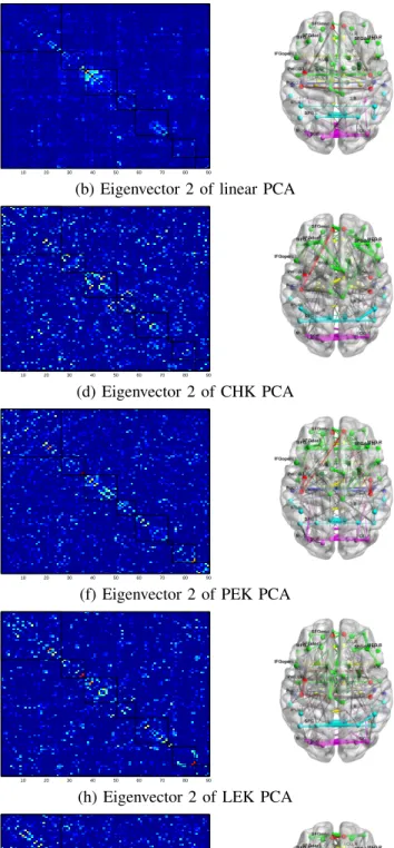
index, and name of each ROI in AAL [41] atlas are listed in Table V. We observe that: i) Compared with the eigenvectors in linear PCA, the eigenvectors obtained in the SPD-kernel PCA capture richer connection structures. Specifically, as seen from Fig. 2(a), the first eigenvector in linear PCA only presents very weak intra-lobe connections in frontal and occipital lobes. In contrast, the first eigenvector obtained by each of the SPD-kernel PCA well captures the intra-lobe connections in all the lobes. Especially, as indicated in Fig. 2(c), (e), (g) and (i), there are strong connections at orbitofrontal cortex ( ROI index: 8, 19-22), rectus gyrus (23, 24), occipital gyrus (43-48), temporal gyri (53-58), Hippocampus (65-66) and temporal pole (69-72). Respecting the second eigenvector, the eigenvectors obtained by the SPD-kernels PCA (Fig. 2(d), (f), (h) and (j)) incorporate both intra-lobe and inter-lobe connections while the eigenvector in linear PCA (Fig. 2(b)) mainly captures only intra-lobe connections in occipital lobe; ii) The pre-images obtained when different SPD kernels are used, as seen in Fig. 2(c)-(j), are very similar with each other
10 20 30 40 50 60 70 80 90 frontal parietal occipital temporal limbic insula sub cortical central 0.01 0.02 0.03 0.04 0.05 0.06 0.07 10 20 30 40 50 60 70 80 90 frontal parietal occipital temporal limbic insula sub cortical central
(a) Eigenvector 1 of linear PCA (b) Eigenvector 2 of linear PCA
10 20 30 40 50 60 70 80 90 frontal parietal occipital temporal limbic insula sub cortical central 0.2 0.4 0.6 0.8 1 1.2 10 20 30 40 50 60 70 80 90 frontal parietal occipital temporal limbic insula sub cortical central
(c) Eigenvector 1 of CHK PCA (d) Eigenvector 2 of CHK PCA
10 20 30 40 50 60 70 80 90 frontal parietal occipital temporal limbic insula sub cortical central 0 0.2 0.4 0.6 0.8 1 1.2 1.4 1.6 10 20 30 40 50 60 70 80 90 frontal parietal occipital temporal limbic insula sub cortical central
(e) Eigenvector 1 of PEK PCA (f) Eigenvector 2 of PEK PCA
10 20 30 40 50 60 70 80 90 frontal parietal occipital temporal limbic insula sub cortical central 0 0.5 1 1.5 10 20 30 40 50 60 70 80 90 frontal parietal occipital temporal limbic insula sub cortical central
(g) Eigenvector 1 of LEK PCA (h) Eigenvector 2 of LEK PCA
10 20 30 40 50 60 70 80 90 frontal parietal occipital temporal limbic insula sub cortical central 0.2 0.4 0.6 0.8 1 1.2 1.4 10 20 30 40 50 60 70 80 90 frontal parietal occipital temporal limbic insula sub cortical central
(i) Eigenvector 1 of SK PCA (j) Eigenvector 2 of SK PCA
Fig. 2. The top two eigenvectors extracted in linear PCA (The first row), CHK PCA (The second row), PEK PCA (The third row), LEK PCA (The fourth row) and LEK PCA (The fifth row).
with slight variation. This is expected since they all reflect the underlying manifold structure of SICE matrices. Further exploration of their clinical interpretation will be included in
0.1 0.5 1 1.5 2 2.5 3 3.5 4 4.5 20 40 60 80 100 120 140 160 180 200 Noise scale δ KL Divergence KL(Σ−1,S) (Original) KL(Σ−1, ˆS)(CHK, proposed) KL(Σ−1, ˆS)(PEK, proposed) KL(Σ−1, ˆS)(LEK, proposed) KL(Σ−1, ˆS)(SK, proposed) 1 2 5 10 20 30 40 50 60 70 8.94 8.96 8.98 9 9.02 9.04 9.06 9.08 9.1 9.12 9.14
The number of top eigenvectors, m
K L ( Σ − 1, S ) -K L ( Σ − 1, ˆS) 5 10 20 30 40 8 8.5 9 9.5
The number of neighbors, L
K L ( Σ − 1, S ) -K L ( Σ − 1, ˆS) (a) (b) (c)
Fig. 3. The performance of the proposed pre-image method on synthetic data set. (a) The averaged KL divergence between the ground truth inverse covariance matrixΣ−1and the original SICE matrixS(labeled by ’original’) or the pre-imagesSˆ when four SPD kernels are used (labeled by ’CHK’, ’PEK’, ’LEK’
and ’SK’, respectively) at various noise levels withmandLset as5and20, respectively. As indicated, the resulting KL divergence values corresponding to the four SPD kernels are consistently smaller thanKL(Σ−1,S)at all noise levels. Moreover, the improvement ofKL(Σ−1,Sˆ)overKL(Σ−1,S), i.e.KL(Σ−1,S)−KL(Σ−1,Sˆ), becomes more significant with increase ofδ. Note that the KL divergence values corresponding to the four kernels are
similar and overlapped in the figure; (b) The improvement of the proposed pre-image method (using Stein kernel) with various number of leading eigenvectors
mwhenLis set as20, and (c) The improvement of the proposed pre-image method (using Stein kernel) with various number of neighborsLwhenmis set as5. 10 20 30 40 50 60 70 80 90 10 20 30 40 50 60 70 80 90 −0.3 −0.2 −0.1 0 0.1 0.2 0.3 10 20 30 40 50 60 70 80 90 10 20 30 40 50 60 70 80 90 −0.3 −0.2 −0.1 0 0.1 0.2 0.3 10 20 30 40 50 60 70 80 90 10 20 30 40 50 60 70 80 90 −0.3 −0.2 −0.1 0 0.1 0.2 0.3 (a) (b) (c)
Fig. 4. Illustration of the result obtained by our proposed pre-image method. (a) shows a ground truth inverse covariance matrixΣ−1, (b) plots the original
SICE matrixSand (c) shows the estimated pre-imageSˆ ofΦm(S). As seen,Sˆis more similar toΣ−1in comparison withS, indicating that the proposed pre-image method brings some kind of denoising effect.
C. Evaluation of The Pre-image Method Using Synthetic Data
To further investigate the efficacy of the proposed pre-image method, a synthetic data set is specially designed for evaluation. The synthetic data set is used for two purposes: i) It allows the comparison between the recovered pre-image of
Φm(·)and the ground truth inverse covariance matrix, which
is not available for real rs-fMRI data; ii) By adjusting the parameters used to generate the synthetic data, the behavior of the proposed pre-image method can be demonstrated. The synthetic data are generated by mimicking the following data generation process in practice.
1) Generate a set of 82 covariance matrices of the size of
90×90, by sampling a Wishart distribution6 [44]. Let
Σi (i = 1,· · ·,82) be the i-th covariance matrix and
its inverse Σ−1i will be used as a ground truth inverse
6The Wishart distribution is used asΣ
i ∼ W90(Σ0, n), whereΣ0 ∈
Sym+90is set as a block-wise covariance matrix for a better illustration of the result, andnis the degree of freedom set as1000.
covariance matrix;
2) A set of 130 vectors are randomly sampled from each
normal distribution N(0,Σi), where i= 1,· · · ,82;
3) Gaussian noise is added to each set of 130 vectors to
simulate that the data are contaminated. The noise level
is denoted byδ;
4) A sample-based covariance matrix C is computed by
using each set of the (noisy)130vectors and82
covari-ance matrices are obtained in total. They are denoted as
C1,C1,· · ·,C82;
5) Apply the SICE method to eachCi to obtain the SICE
matrix, and they are collectively denoted by {Si}82i=1.
These SICE matrices form the synthetic data set. Note that they are affected by the noise added in Step 3. From the synthetic data set {Si}82i=1, every Si is selected
in turn as the test data and the remainder are used as the training set. Algorithm 1 is then applied to estimate the
pre-imageSˆi for Φm(Si). Then the recovered pre-image Sˆi and
truth inverse covariance matrix Σ−1i prepared in Step 1. This is to see whetherSˆiis really closer toΣ−1i thanSi. Following
the literature [45], we use Kullback-Liebler (KL) divergence
to compare Sˆi (or Si) with Σ−1i . Given a pair of SPD
matrices Σ1 andΣ2, KL divergence measures the similarity
of two GaussiansN(µ1,Σ1)andN(µ2,Σ2). It can be used
to measure the similarity between the two SPD matrices by relating them to the covariance matrices and setting the means as zero. KL divergence in our case is expressed as
KL(Σ1,Σ2) = tr(Σ−12 Σ1)−log det(Σ−12 Σ1)−d, where
d is the number of network nodes. It is nonnegative and a
smaller divergence indicates that these two matrices are more similar.
The result is shown in Fig. 3. As seen in Fig. 3(a),
KL(Σ−1,Sˆ)(averaged over all82test cases and withmand
L set as 5 and 20, respectively.) is consistently lower than
KL(Σ−1,S) for all the different noise levels and the SPD
kernels used in the kernel PCA. This result suggests that the
obtained pre-image Sˆ is closer to the ground truth inverse
covariance matrix Σ−1 in comparison with the original SICE
matrix S. Relating back to the idea that we use to design
this experiment, this result shows that the proposed pre-image
method indeed works. Also, the improvement ofKL(Σ−1,Sˆ)
overKL(Σ−1,S), i.e.KL(Σ−1,S)−KL(Σ−1,Sˆ), becomes
more significant with the increase of the noise level δ
in-troduced in Step 3 of the synthetic data generation process. To demonstrate the result obtained by the proposed pe-image method, an example is given in Fig. 4, where Fig. 4(a) shows
a ground truth inverse covariance matrix Σ−1, Fig. 4(b) plots
the estimated SICE matrix S and Fig. 4(c) shows the
pre-image Sˆ of Φm(S). As seen, Sˆ is more similar to Σ−1 in
comparison withS.
As indicated in Algorithm 1, the number of leading
eigen-vectors mand the number of neighbors Lare two important
parameters. We evaluate how the performance of the proposed pre-image method will change with these two parameters. Stein kernel is taken as an example. Fig. 3(b) and Fig. 3(c)
show the improvement, i.e. KL(Σ−1,S)−KL(Σ−1,Sˆ), of
our method with different m andL, respectively. As seen in
Fig. 3(b), when Lis set as constant20, the improvement first
increases with m and then decreases, achieving the highest
value whenmis five. This is because the first several leading
eigenvectorsviinFrepresent the dominant network structures
of the network while the following ones intend to characterize more detailed structures which are vulnerable to noise. As
a result, with the increasing value of m, the components
often correspond to noise. Therefore, when m > 5, noisy
components could be included, and this reduces the magni-tude of the improvement. At the same time, note that the improvement does consistently hold although its magnitude
is reduced. Fig. 3(c) shows that, when m is fixed at 5, the
improvement with the increase ofL becomes saturated when
L = 20. This is because the constraint of PL
j=1wj = 1
in Sˆ = PL
j=1wjSj (Eq.(11)) imposes the sparsity of wj,
limiting the actual number of neighborsSj used to estimateSˆ.
Based on our experience, a relatively large initial number of
L is recommended, e.g. one fourth of the number of training
samples, and the constraint of PL
j=1wj = 1 will implicitly
and automatically select a small set ofSj by setting mostwj
as zero.
TABLE V
THE NAME AND LOBE OF EACHROIINFIG. (2).
Lobe ROI
in-dex
ROI name ROI
in-dex
ROI name
frontal
1 Frontal Sup L 2 Frontal Sup R 3 Frontal Sup Orb L 4 Frontal Sup Orb R 5 Frontal Mid L 6 Frontal Mid R 7 Frontal Mid Orb L 8 Frontal Mid Orb R 9 Frontal Inf Oper L 10 Frontal Inf Oper R 11 Frontal Inf Tri L 12 Frontal Inf Tri R 13 Frontal Inf Orb L 14 Frontal Inf Orb R 15 Supp Motor Area L 16 Supp Motor Area R 17 Olfactory L 18 Olfactory R
19 Frontal Sup Medial L 20 Frontal Sup Medial R 21 Frontal Mid Orb L 22 Frontal Mid Orb R
23 Rectus L 24 Rectus R
25 Paracentral Lobule L 26 Paracentral Lobule R
parietal
27 Parietal Sup L 28 Parietal Sup R 29 Parietal Inf L 30 Parietal Inf R 31 SupraMarginal L 32 SupraMarginal R 33 Angular L 34 Angular R 35 Precuneus L 36 Precuneus R occipital 37 Calcarine L 38 Calcarine R 39 Cuneus L 40 Cuneus R 41 Lingual L 42 Lingual R
43 Occipital Sup L 44 Occipital Sup R 45 Occipital Mid L 46 Occipital Mid R 47 Occipital Inf L 48 Occipital Inf R
49 Fusiform L 50 Fusiform R
temporal
51 Heschl L 52 Heschl R
53 Temporal Sup L 54 Temporal Sup R 55 Temporal Mid L 56 Temporal Mid R 57 Temporal Inf L 58 Temporal Inf R
limbic
59 Cingulum Ant L 60 Cingulum Ant R 61 Cingulum Mid L 62 Cingulum Mid R 63 Cingulum Post L 64 Cingulum Post R 65 Hippocampus L 66 Hippocampus R 67 ParaHippocampal L 68 ParaHippocampal R 69 Temporal Pole Sup L 70 Temporal Pole Sup R 71 Temporal Pole Mid L 72 Temporal Pole Mid R
insula 73 Insula L 74 Insula R
sub cortical 75 Amygdala L 76 Amygdala R 77 Caudate L 78 Caudate R 79 Putamen L 80 Putamen R 81 Pallidum L 82 Pallidum R 83 Thalamus L 84 Thalamus R central 85 Precentral L 86 Precentral R 87 Rolandic Oper L 88 Rolandic Oper R 89 Postcentral L 90 Postcentral R
V. CONCLUSION
Recently, sparse inverse covariance matrix (SICE) has been used as a representation of brain connectivity to classify Alzheimer’s disease and normal controls. However, its high dimensionality can adversely affect the classification per-formance. Taking advantage of the SPD property of SICE matrices, we use SPD-kernel PCA to extract principal com-ponents to obtain a compact representation for classification. We also propose a pre-image estimation algorithm, which allows visualization and analysis of the extracted principal connectivity patterns in the input space. The efficacy of the proposed method is verified by extensive experimental study on synthetic data and real rs-fMRI data from the ADNI.
In this paper, we specifically focus on unsupervised learning to explore compact representation without using class label information. Note that our framework can readily be extended to supervised case, such as kernel linear discriminant analysis (KLDA), to explore discriminative representation. This will be studied in our future work.
REFERENCES
[1] T. Mushaet al., “EEG markers for characterizing anomalous activities of cerebral neurons in nat (neuronal activity topography) method,” Biomedical Engineering, IEEE Transactions on, vol. 60, no. 8, pp. 2332– 2338, 2013.
[2] C. Jacket al., “Prediction of ad with mri-based hippocampal volume in mild cognitive impairment,”Neurology, vol. 52, no. 7, pp. 1397–1397, 1999.
[3] J. Richiardi et al., “Classifying minimally disabled multiple sclerosis patients from resting state functional connectivity,”NeuroImage, vol. 62, no. 3, pp. 2021–2033, 2012.
[4] R. Gouldet al., “Brain mechanisms of successful compensation during learning in alzheimer disease,”Neurology, vol. 67, no. 6, pp. 1011–1017, 2006.
[5] X. Yanget al., “Evaluation of statistical inference on empirical resting state fMRI,”Biomedical Engineering, IEEE Transactions on, vol. 61, no. 4, pp. 1091–1099, April 2014.
[6] G. Varoquaux et al., “Detection of brain functional-connectivity dif-ference in post-stroke patients using group-level covariance modeling,” in Medical Image Computing and Computer-Assisted Intervention– MICCAI 2010. Springer, 2010, pp. 200–208.
[7] K. Ugurbil, “Magnetic resonance imaging at ultrahigh fields,” Biomedi-cal Engineering, IEEE Transactions on, vol. 61, no. 5, pp. 1364–1379, May 2014.
[8] V. D. Heuvelet al., “Exploring the brain network: a review on resting-state fMRI functional connectivity,”European Neuropsychopharmacol-ogy, vol. 20, no. 8, pp. 519–534, 2010.
[9] R. L. Buckner and J. L. Vincent, “Unrest at rest: default activity and spontaneous network correlations,” Neuroimage, vol. 37, no. 4, pp. 1091–1096, 2007.
[10] M. D. Greiciuset al., “Functional connectivity in the resting brain: a network analysis of the default mode hypothesis,”Proceedings of the National Academy of Sciences, vol. 100, no. 1, pp. 253–258, 2003. [11] V. Calhoun et al., “A method for making group inferences from
functional mri data using independent component analysis,” Human brain mapping, vol. 14, no. 3, pp. 140–151, 2001.
[12] S. B. Katwalet al., “Unsupervised spatiotemporal analysis of fMRI data using graph-based visualizations of self-organizing maps,”Biomedical Engineering, IEEE Transactions on, vol. 60, no. 9, pp. 2472–2483, 2013. [13] J. Damoiseauxet al., “Consistent resting-state networks across healthy subjects,”Proceedings of the National Academy of Sciences, vol. 103, no. 37, pp. 13 848–13 853, 2006.
[14] M. van den Heuvelet al., “Normalized cut group clustering of resting-state fmri data,”PloS one, vol. 3, no. 4, p. e2001, 2008.
[15] S. M. Smithet al., “Functional connectomics from resting-state fMRI,” Trends in cognitive sciences, vol. 17, no. 12, pp. 666–682, 2013. [16] N. Leonardi et al., “Principal components of functional connectivity:
A new approach to study dynamic brain connectivity during rest,” NeuroImage, vol. 83, pp. 937–950, 2013.
[17] C.-Y. Weeet al., “Constrained sparse functional connectivity networks for MCI classification,” in Medical Image Computing and Computer-Assisted Intervention–MICCAI 2012. Springer, 2012, pp. 212–219. [18] S. M. Smith, “The future of fMRI connectivity,”Neuroimage, vol. 62,
no. 2, pp. 1257–1266, 2012.
[19] J. Friedman et al., “Sparse inverse covariance estimation with the graphical lasso,”Biostatistics, vol. 9, no. 3, pp. 432–441, 2008. [20] S. Huanget al., “Learning brain connectivity of alzheimers disease by
exploratory graphical models,”NeuroImage, vol. 50, pp. 935–949, 2010. [21] ——, “Learning brain connectivity of alzheimer’s disease by sparse inverse covariance estimation,” NeuroImage, vol. 50, no. 3, pp. 935– 949, 2010.
[22] B. Nget al., “A novel sparse group gaussian graphical model for func-tional connectivity estimation,” inInformation Processing in Medical Imaging. Springer, 2013, pp. 256–267.
[23] O. Sporns et al., “Identification and classification of hubs in brain networks,”PloS one, vol. 2, no. 10, p. e1049, 2007.
[24] X. Pennec et al., “A riemannian framework for tensor computing,” International Journal of Computer Vision, vol. 66, no. 1, pp. 41–66, 2006.
[25] P. T. Fletcher et al., “Principal geodesic analysis for the study of nonlinear statistics of shape,”Medical Imaging, IEEE Transactions on, vol. 23, no. 8, pp. 995–1005, 2004.
[26] S. Sra, “Positive definite matrices and the symmetric stein divergence,” arXiv preprint arXiv:1110.1773, 2011.
[27] V. Arsigny et al., “Log-euclidean metrics for fast and simple calculus on diffusion tensors,” Magnetic Resonance in Medicine, vol. 56, no. 2, pp. 411–421, 2006. [Online]. Available: http://dx.doi.org/10.1002/mrm.20965
[28] M. T. Harandi et al., “Sparse coding and dictionary learning for symmetric positive definite matrices: A kernel approach,” inComputer Vision–ECCV 2012. Springer, 2012, pp. 216–229.
[29] S. Jayasumanaet al., “Kernel methods on the riemannian manifold of symmetric positive definite matrices,” inComputer Vision and Pattern Recognition, IEEE Computer Society Conference on, 2013.
[30] J.-Y. Kwok and I.-H. Tsang, “The pre-image problem in kernel meth-ods,”Neural Networks, IEEE Transactions on, vol. 15, no. 6, pp. 1517– 1525, 2004.
[31] Y. Rathiet al., “Statistical shape analysis using kernel PCA,” in Elec-tronic Imaging 2006. International Society for Optics and Photonics, 2006, pp. 60 641B–60 641B.
[32] S. M. Smithet al., “Network modelling methods for fmri,”Neuroimage, vol. 54, no. 2, pp. 875–891, 2011.
[33] J. Zhanget al., “Exploring compact representation of SICE matrices for functional brain network classification,”MICCAI Workshop on Machine Learning in Medical Imaging (MLMI), Boston, USA, 2014.
[34] J. Liu et al., SLEP: Sparse Learning with Efficient Projections, Arizona State University, 2009. [Online]. Available: http://www.public.asu.edu/ jye02/Software/SLEP
[35] W. F¨orstner and B. Moonen, “A metric for covariance matrices,” in Geodesy-The Challenge of the 3rd Millennium. Springer, 2003, pp. 299–309.
[36] I. L. Drydenet al., “Non-euclidean statistics for covariance matrices, with applications to diffusion tensor imaging,”The Annals of Applied Statistics, pp. 1102–1123, 2009.
[37] B. Sch¨olkopfet al., “Nonlinear component analysis as a kernel eigen-value problem,” Neural computation, vol. 10, no. 5, pp. 1299–1319, 1998.
[38] L. Zhou et al., “Identifying anatomical shape difference by regular-ized discriminative direction,”Medical Imaging, IEEE Transactions on, vol. 28, no. 6, pp. 937–950, 2009.
[39] O. Tuzelet al., “Pedestrian detection via classification on riemannian manifolds,”Pattern Analysis and Machine Intelligence, IEEE Transac-tions on, vol. 30, no. 10, pp. 1713–1727, 2008.
[40] Y. Chao-Gan and Z. Yu-Feng, “DPARSF: a matlab toolbox for pipeline data analysis of resting-state fMRI,”Frontiers in systems neuroscience, vol. 4, 2010.
[41] N. Tzourio-Mazoyeret al., “Automated anatomical labeling of activa-tions in spm using a macroscopic anatomical parcellation of the MNI MRI single-subject brain,” Neuroimage, vol. 15, no. 1, pp. 273–289, 2002.
[42] M. Kaiser, “A tutorial in connectome analysis: topological and spatial features of brain networks,”Neuroimage, vol. 57, no. 3, pp. 892–907, 2011.
[43] S. Mika et al., “Kernel PCA and de-noising in feature spaces,” in Proceedings of the 1998 Conference on Advances in Neural Information Processing Systems II. Cambridge, MA, USA: MIT Press, 1999, pp. 536–542. [Online]. Available: http://dl.acm.org/citation.cfm?id=340534.340729
[44] T. Tokudaet al., “Visualizing distributions of covariance matrices,” Tech. Rep., 2011.
[45] N. St¨adler and P. B¨uhlmann, “Missing values: sparse inverse covari-ance estimation and an extension to sparse regression,”Statistics and Computing, vol. 22, no. 1, pp. 219–235, 2012.
![Fig. 1. The illustration of the Riemannian manifold of SPD matrices. (a) Sym + d forms a closed, self-dual convex cone, which is a Riemannian manifold in the Euclidean space R d×d [26]](https://thumb-us.123doks.com/thumbv2/123dok_us/10055517.2905262/5.918.471.836.104.262/illustration-riemannian-manifold-matrices-closed-riemannian-manifold-euclidean.webp)