Grassmann Discriminant Analysis: a Unifying View on Subspace-Based Learning

University of Pennsylvania

ScholarlyCommons

Departmental Papers (ESE)

Department of Electrical & Systems Engineering

July 2008

Grassmann Discriminant Analysis: a Unifying

View on Subspace-Based Learning

Jihun Hamm

University of Pennsylvania

Daniel D. Lee

University of Pennsylvania, [email protected]

Follow this and additional works at:

http://repository.upenn.edu/ese_papers

Reprinted from the Proceedings of the 25th International Conference on Machine Learning (ICML 2008), July 2008. URL: http://icml2008.cs.helsinki.fi/index.shtml

This paper is posted at ScholarlyCommons.http://repository.upenn.edu/ese_papers/465 For more information, please [email protected].

Recommended Citation

Grassmann Discriminant Analysis: a Unifying View on Subspace-Based

Learning

Abstract

In this paper we propose a discriminant learning framework for problems in which data consist of linear

subspaces instead of vectors. By treating subspaces as basic elements, we can make learning algorithms adapt

naturally to the problems with linear invariant structures. We propose a unifying view on the subspace-based

learning method by formulating the problems on the Grassmann manifold, which is the set of

fixed-dimensional linear subspaces of a Euclidean space. Previous methods on the problem typically adopt an

inconsistent strategy: feature extraction is performed in the

Euclidean

space while

non-Euclidean

distances are

used. In our approach, we treat each subspace as a point in the Grassmann space, and perform feature

extraction and classification in the same space. We show feasibility of the approach by using the Grassmann

kernel functions such as the Projection kernel and the Binet-Cauchy kernel. Experiments with real image

databases show that the proposed method performs well compared with state-of- the-art algorithms.

Reprinted from the Proceedings of the 25th International Conference on Machine Learning (ICML 2008),

July 2008.

URL: http://icml2008.cs.helsinki.fi/index.shtml

Grassmann Discriminant Analysis:

a Unifying View on Subspace-Based Learning

Jihun Hamm _{[email protected]}

Daniel D. Lee _{[email protected]}

GRASP Laboratory, University of Pennsylvania, Philadelphia, PA 19104 USA

Abstract

In this paper we propose a discriminant learning framework for problems in which data consist of linear subspaces instead of vectors. By treating subspaces as basic el-ements, we can make learning algorithms adapt naturally to the problems with lin-ear invariant structures. We propose a uni-fying view on the subspace-based learning method by formulating the problems on the Grassmann manifold, which is the set of fixed-dimensional linear subspaces of a Eu-clidean space. Previous methods on the prob-lem typically adopt an inconsistent strategy:

feature extraction is performed in the

Eu-clidean space while non-Euclidean distances are used. In our approach, we treat each sub-space as a point in the Grassmann sub-space, and perform feature extraction and classification

in the same space. We show feasibility of

the approach by using the Grassmann kernel functions such as the Projection kernel and the Binet-Cauchy kernel. Experiments with real image databases show that the proposed method performs well compared with state-of-the-art algorithms.

1. Introduction

We often encounter learning problems in which the

ba-sic elements of the data aresets of vectors instead of

vectors. Suppose we want to recognize a person from multiple pictures of the individual, taken from differ-ent angles, under differdiffer-ent illumination or at differdiffer-ent places. When comparing such sets of image vectors, we are free to define the similarity between sets based on Appearing inProceedings of the 25thInternational Confer-ence on Machine Learning, Helsinki, Finland, 2008. Copy-right 2008 by the author(s)/owner(s).

the similarity between image vectors (Shakhnarovich et al., 2002; Kondor & Jebara, 2003; Zhou & Chel-lappa, 2006).

In this paper, we specifically focus on those data that can be modeled as a collection of linear subspaces. In the example above, let’s assume that the set of images of a single person is well approximated by a low di-mensional subspace (Turk & Pentland, 1991), and the whole data is the collection of such subspaces. The benefits of using subspaces are two-fold: 1) compar-ing two subspaces is cheaper than comparcompar-ing two sets directly when those sets are very large, and 2) it is more robust to missing data since the subspace can ‘fill-in’ the missing pictures. However the advantages come with the challenge of representing and handling the subspaces appropriately.

We approach the subspace-based learning problems by formulating the problems on the Grassmann manifold, the set of fixed-dimensional linear subspaces of a Eu-clidean space. With this unifying framework we can make analytic comparisons of the various distances of subspaces. In particular, we single out those distances

that are induced from the Grassmann kernels, which

are positive definite kernel functions on the Grassmann

space. The Grassmann kernels allow us to use the

usual kernel-based algorithms on this unconventional space and to avoid ad hoc approaches to the problem. We demonstrate the proposed framework by using the Projection metric and the Binet-Cauchy metric and by applying kernel Linear Discriminant Analysis to clas-sification problems with real image databases.

1.1. Contributions of the Paper

Although the Projection metric and the Binet-Cauchy metric were previously used (Chang et al., 2006; Wolf & Shashua, 2003), their potential for subspace-based learning has not been fully explored. In this work, we provide an analytic exposition of the two metrics as examples of the Grassmann kernels, and contrast the

Yi Yj θ 2

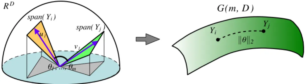
G(m, D)

Figure 1.Principal angles and Grassmann distances. Let span(Yi) and span(Yj) be two subspaces in the Euclidean space

RD on the left. The distance between two subspaces span(Yi) and span(Yj) can be measured by the principal angles θ= [θ1, ... , θm]0 using the usual innerproduct of vectors. In the Grassmann manifold viewpoint, the subspaces span(Yi)

and span(Yj) are considered as two points on the manifoldG(m, D), whose Riemannian distance is related to the principal

angles byd(Yi, Yj) =kθk2. Various distances can be defined based on the principal angles.

two metrics with other metrics used in the literature. Several subspace-based classification methods have been previously proposed (Yamaguchi et al., 1998; Sakano, 2000; Fukui & Yamaguchi, 2003; Kim et al., 2007). However, these methods adopt an inconsistent

strategy: feature extraction is performed in the

Eu-clideanspace when non-Euclideandistances are used. This inconsistency can result in complications and

weak guarantees. In our approach, the feature

ex-traction and the distance measurement are integrated around the Grassmann kernel, resulting in a simpler and better-understood formulation.

The rest of the paper is organized as follows. In Sec. 2 and 3 we introduce the Grassmann manifolds and

de-rive various distances on the space. In Sec. 4 we

present a kernel view of the problem and emphasize the advantages of using positive definite metrics. In Sec. 5 we propose the Grassmann Discriminant Analysis and compare it with other subspace-based discrimination methods. In Sec. 6 we test the proposed algorithm for face recognition and object categorization tasks. We conclude in Sec. 7 with a discussion.

2. Grassmann Manifold and Principal

Angles

In this section we briefly review the Grassmann man-ifold and the principal angles.

Definition 1 The Grassmann manifold G(m, D) is the set of m-dimensional linear subspaces of the_RD_.

TheG(m, D) is am(D−m)-dimensional compact

Rie-mannian manifold.1 An element of G(m, D) can be

1_{G(m, D) can be derived as a quotient space of}

orthog-onal groups G(m, D) =O(D)/O(m)× O(D−m), where

represented by an orthonormal matrixY of size Dby

msuch thatY0Y =Im, whereImis thembym

iden-tity matrix. For example,Y can be thembasis vectors

of a set of pictures in RD. However, the matrix

rep-resentation of a point in G(m, D) is not unique: two

matricesY1andY2are considered the same if and only

if span(Y1) = span(Y2), where span(Y) denotes the

subspace spanned by the column vectors ofY.

Equiva-lently, span(Y1) = span(Y2) if and only ifY1R1=Y2R2

for someR1, R2∈ O(m). With this understanding, we

will often use the notation Y when we actually mean

its equivalence class span(Y), and use Y1 =Y2 when

we mean span(Y1) = span(Y2), for simplicity.

Formally, the Riemannian distance between two sub-spaces is the length of the shortest geodesic connecting the two points on the Grassmann manifold. However, there is a more intuitive and computationally efficient

way of defining the distances using theprincipal angles

(Golub & Loan, 1996).

Definition 2 Let Y1 and Y2 be two orthonormal

matrices of size D by m. The principal an-gles 0≤θ1≤ · · · ≤θm≤π/2 between two subspaces

span(Y1)and span(Y2), are defined recursively by

cosθk= max uk∈span(Y1) max vk∈span(Y2) uk0vk, subject to uk0uk = 1, vk0vk= 1, uk0ui= 0, vk0vi= 0, (i= 1, ..., k−1).

In other words, the first principal angleθ1is the small-est angle between all pairs of unit vectors in the first and the second subspaces. The rest of the principal

O(m) is the group ofmbym orthonormal matrices. We refer the readers to (Wong, 1967; Absil et al., 2004) for details on the Riemannian geometry of the space.

Grassmann Discriminant Analysis

angles are similarly defined. It is known (Wong, 1967; Edelman et al., 1999) that the principal angles are

re-lated to the geodesic distance by d2

G(Y1, Y2) = P_iθ2i

(refer to Fig. 1.)

The principal angles can be computed from the Singu-lar Value Decomposition (SVD) ofY₁0Y2,

Y₁0Y2=U(cos Θ)V0, (1)

where U = [u1 ... um], V = [v1 ... vm], and cos Θ

is the diagonal matrix cos Θ = diag(cosθ1 ... cosθm).

The cosines of the principal angles cosθ1, ... ,cosθm

are also known ascanonical correlations.

Although the definition can be extended to the cases

where Y1 and Y2 have different number of columns,

we will assumeY1 andY2 have the same sizeD bym

throughout this paper. Also, we will occasionally use G instead ofG(m, D) for simplicity.

3. Distances for Subspaces

In this paper we use the term distance as any

assign-ment of nonnegative values for each pair of points in

a spaceX. A validmetricis, however, a distance that

satisfies the additional axioms:

Definition 3 A real-valued function d:X × X →R

is called a metric if 1. d(x1, x2)≥0, 2. d(x1, x2) = 0if and only if x1=x2, 3. d(x1, x2) =d(x2, x1), 4. d(x1, x2) +d(x2, x3)≤d(x1, x3), for allx1, x2, x3∈ X.

A distance (or a metric) between subspacesd(Y1, Y2) has to be invariant under different representations

d(Y1, Y2) =d(Y1R1, Y2R2), ∀R1, R2∈ O(m).

In this section we introduce various distances for sub-spaces derivable from the principal angles.

3.1. Projection Metric and Binet-Cauchy Metric

We first underline two main distances of this paper. 1. Projection metric dP(Y1, Y2) = m X i=1 sin2θi !1/2 = m− m X i=1 cos2θi !1/2 . (2)

The Projection metric is the 2-norm of the sine of principal angles (Edelman et al., 1999; Wang et al., 2006). 2. Binet-Cauchy metric dBC(Y1, Y2) = 1− Y i cos2θi !1/2 . (3)

The Binet-Cauchy metric is defined with the

product of canonical correlations (Wolf &

Shashua, 2003; Vishwanathan & Smola, 2004). As the names hint, these two distances are in fact valid metrics satisfying Def. 3. The proofs are deferred until Sec. 4.

3.2. Other Distances in the Literature

We describe a few other distances used in the liter-ature. The principal angles are the keys that relate these distances.

1. Max Correlation

dMax(Y1, Y2) = 1−cos2θ1

1/2

= sinθ1. (4) The max correlation is a distance based on only

the largest canonical correlation cosθ1 (or the

smallest principal angle θ1). This max

correla-tion was used in previous works (Yamaguchi et al., 1998; Sakano, 2000; Fukui & Yamaguchi, 2003). 2. Min Correlation

dMin(Y1, Y2) = 1−cos2θm

1/2

= sinθm. (5)

The min correlation is defined similarly to the

max correlation. However, the min correlation

is more closely related to the Projection metric:

we can rewrite the Projection metric as dP =

2−1/2 _kY

1Y10 −Y2Y20kF and the min correlation

asdMin=kY1Y10−Y2Y20k2. 3. Procrustes metric dCF(Y1, Y2) = 2 m X i=1 sin2(θi/2) !1/2 . (6)

The Procrustes metric is the minimum distance between different representations of two subspaces span(Y1) and span(Y2): (Chikuse, 2003)

dCF = min

R1,R2∈O(m)

kY1R1−Y2R2kF =kY1U−Y2VkF,

where U and V are from (1). By definition,

bases of span(Y1) and span(Y2). The Procrustes metric is also called chordal distance (Edelman et al., 1999). We can similarly define the mini-mum distance using other matrix norms such as

dC2(Y1, Y2) =kY1U−Y2Vk2= 2 sin(θm/2).

3.3. Which Distance to Use?

The choice of the best distance for a classification task depends on a few factors. The first factor is the dis-tribution of data. Since the distances are defined with particular combinations of the principal angles, the best distance depends highly on the probability dis-tribution of the principal angles of the given data. For example,dMaxuses the smallest principal angleθ1 only, and may be robust when the data are noisy. On the other hand, when all subspaces are sharply concen-trated on one point,dMaxwill be close to zero for most

of the data. In this case, dMin may be more

discrimi-native. The Projection metric dP, which uses all the

principal angles, will show intermediate characteristics between the two distances. Similar arguments can be

made for the Procrustes metrics dCF and dC2, which

use all angles and the largest angle only, respectively. The second criterion for choosing the distance, is the degree of structure in the distance. Without any struc-ture a distance can be used only with a simple K-Nearest Neighbor (K-NN) algorithm for classification. When a distance have an extra structure such as tri-angle inequality, for example, we can speed up the nearest neighbor searches by estimating lower and

up-per limits of unknown distances (Farag´o et al., 1993).

From this point of view, the max correlation is not a metric and may not be used with more sophisticated algorithms. On the other hand, the Min Correlation

and the Procrustes metrics are valid metrics2_.

The most structured metrics are those which are in-duced from a positive definite kernel. Among the met-rics mentioned so far, only the Projection metric and

the Binet-Cauchy metric belong to this class. The

proof and the consequences of positive definiteness are the main topics of the next section.

4. Kernel Functions for Subspaces

We have defined a valid metric on Grassmann mani-folds. The next question is whether we can define a kernel function compatible with the metric. For this

purpose let’s recall a few definitions. Let X be any

2_{The metric properties follow from the properties of}

matrix 2-norm and F-norm. To check the conditions in Def. 3 for Procrustes we use the equality minR1,R2 kY1R1−

Y2R2k2,F = minR3kY1−Y2R3k2,F forR1, R2, R3∈ O(m).

set, and k : X × X → _R be a symmetric real-valued

functionk(xi, xj) =k(xj, xi) for allxi, xj∈ X.

Definition 4 A real symmetric function is a (resp. conditionally) positive definite kernel function, if P

i,jcicjk(xi, xj) ≥ 0, for all x1, ..., xn(xi ∈ X) and

c1, ..., cn(ci ∈ R) for any n ∈ N. (resp. for all c1, ..., cn(ci∈R)such that Pni=1ci= 0.)

In this paper we are interested in the kernel functions on the Grassmann space.

Definition 5 A Grassmann kernel function is a pos-itive definite kernel function onG.

In the following we show that the Projection metric and the Binet-Cauchy are induced from the Grass-mann kernels.

4.1. Projection Metric

The Projection metric can be understood by

associ-ating a point span(Y)∈ G with its projection matrix

Y Y0 by an embedding:

ΨP :G(m, D)→RD×D, span(Y)7→Y Y0. (7)

The image ΨP(G(m, D)) is the set of rank-m

or-thogonal projection matrices. This map is in fact

an isometric embedding (Chikuse, 2003) and the projection metric is simply a Euclidean distance in

RD×D. The corresponding innerproduct of the space

is tr [(Y1Y10)(Y2Y20)] =kY10Y2k2F, and therefore

Proposition 1 The Projection kernel

kP(Y1, Y2) =kY10Y2k 2

F (8)

is a Grassmann kernel.

Proof The kernel is well-defined becausekP(Y1, Y2) =

kP(Y1R1, Y2R2) for any R1, R2∈ O(m). The positive definiteness follows from the properties of the Frobe-nius norm. For allY1, ..., Yn(Yi∈ G) andc1, ..., cn(ci∈

R) for anyn∈N, we have

X ij cicjkYi0Yjk2F = X ij cicjtr(YiYi0YjYj0) = tr(X i ciYiYi0) 2 _{= k}X i ciYiYi0k 2 F ≥0.

We can generate a family of kernels from the Projec-tion kernel. For example, the square-root kY_i0YjkF is

Grassmann Discriminant Analysis

4.2. Binet-Cauchy Metric

The Binet-Cauchy metric can also be understood from

an embedding. Let s be a subset of {1, ..., D} with

m elements s ={r1, ..., rm}, and Y(s) be the m×m

matrix whose rows are ther1, ... , rm-th rows ofY. If

s1, s2, ..., snare all such choices of the subsetsordered

lexicographically, then the Binet-Cauchy embedding is defined as

ΨBC :G(m, D)→Rn, Y 7→

detY(s1)_{, ...,detY}(sn)_,

(9)

wheren=DCmis the number of choosingmrows out

of D rows. The natural innerproduct in this case is

Pn r=1detY (si) 1 detY (si) 2 .

Proposition 2 The Binet-Cauchy kernel

kBC(Y1, Y2) = (detY10Y2) 2

= detY10Y2Y20Y1 (10)

is a Grassmann kernel.

Proof First, the kernel is well-defined because

kBC(Y1, Y2) = kBC(Y1R1, Y2R2) for any R1, R2 ∈ O(m). To show thatkBC is positive definite it suffices

to show that k(Y1, Y2) = detY10Y2 is positive definite. From the Binet-Cauchy identity, we have

detY₁0Y2=

X

s

detY₁(s)detY₂(s).

Therefore, for allY1, ..., Yn(Yi ∈ G) andc1, ..., cn(ci ∈

R) for anyn∈N, we have

X ij cicjdetYi0Yj = X ij cicj X s detY_i(s)detY_j(s) = X s X i cidetY (s) i !2 ≥0.

We can also generate another family of kernels

from the Binet-Cauchy kernel. Note that although

detY10Y2 is a Grassmann kernel we prefer using

kBC(Y1, Y2) = det(Y10Y2)2, since it is directly related to principal angles det(Y0

1Y2)2 = Qcos2θi, whereas

detY₁0Y2 6= Qcosθi in general.3 Another variant

arcsinkBC(Y1, Y2) is also a positive definite kernel4 and its induced metric d = (arccos(detY₁0Y2))1/2 is a conditionally positive definite metric.

4.3. Indefinite Kernels from Other Metrics

Since the Projection metric and the Binet-Cauchy metric are derived from positive definite kernels, all

3_detY0

1Y2can be negative whereasQcosθi, the product

of singular values, is nonnegative by definition.

4_{Theorem 4.18 and 4.19 (Sch¨olkopf & Smola, 2001).}

the kernel-based algorithms for Hilbert spaces are at our disposal. In contrast, other metrics in the previ-ous sections are not associated with any Grassmann kernel. To show this we can use the following result (Schoenberg, 1938; Hein et al., 2005):

Proposition 3 A metricdis induced from a positive definite kernel if and only if

ˆ

k(x1, x2) =−d2(x1, x2)/2, x1, x2∈ X (11)

is conditionally positive definite.

The proposition allows us to show a metric’s non-positive definiteness by constructing an indefinite ker-nel matrix from (11) as a counterexample.

There have been efforts to use indefinite kernels for learning (Ong et al., 2004; Haasdonk, 2005), and sev-eral heuristics have been proposed to make an in-definite kernel matrix to a positive in-definite matrix (Pekalska et al., 2002). However, we do not advocate the use of the heuristics since they change the geome-try of the original data.

5. Grassmann Discriminant Analysis

In this section we give an example of the Discriminant Analysis on Grassmann space by using kernel LDA with the Grassmann kernels.

5.1. Linear Discriminant Analysis

The Linear Discriminant Analysis (LDA) (Fukunaga, 1990), followed by a K-NN classifier, has been success-fully used for classification.

Let {x1, ...,xN} be the data vectors and {y1, ..., yN}

be the class labels yi ∈ {1, ..., C}. Without loss of

generality we assume the data are ordered according to the class labels: 1 =y1≤y2≤...≤yN =C. Each

classc hasNc number of samples.

Letµc= 1/NcP_{i|yi=c}xibe the mean of classc, and

µ = 1/NP

ixi be the overall mean. LDA searches

for the discriminant directionw which maximizes the

Rayleigh quotient L(w) = w0Sbw/w0Sww where Sb

andSware the between-class and within-class

covari-ance matrices respectively:

Sb = 1 N C X c=1 Nc(µc−µ)(µc−µ)0 Sw = 1 N C X c=1 X {i|yi=c} (xi−µc)(xi−µc)0

The optimal w is obtained from the largest

eigenvec-tor ofS−1

C−1-number of local optima W = {w1, ...,wC−1}.

By projecting data onto the space spanned by W, we

achieve dimensionality reduction and feature extrac-tion of data onto the most discriminant subspace.

5.2. Kernel LDA with Grassmann Kernels

Kernel LDA can be formulated by using the kernel

trick as follows. Let φ: G → H be the feature map,

and Φ = [φ1...φN] be the feature matrix of the

train-ing points. Assumtrain-ingwis a linear combination of the

those feature vectors, w = Φα, we can rewrite the

Rayleigh quotient in terms ofαas

L(α) = α 0_Φ0_S BΦα α0_Φ0_S WΦα = α 0_{K(V −1} N10N/N)Kα α0_(K(I N −V)K+σ2IN)α , (12)

where K is the kernel matrix, 1N is a uniform vector

[1 ... 1]0 of length N, V is a block-diagonal matrix

whose c-th block is the uniform matrix 1Nc1

0

Nc/Nc,

andσ2_I

N is a regularizer for making the computation

stable. Similarly to LDA, the set of optimal α’s are

computed from the eigenvectors.

The procedures for using kernel LDA with the Grass-mann kernels are summarized below:

Assume the D by m orthonormal bases {Yi} are

already computed from the SVD of sets in the data. Training:

1. Compute the matrix [Ktrain]ij =kP(Yi, Yj) or

kBC(Yi, Yj)for allYi, Yj in the training set.

2. Solve max_α L(α)by eigen-decomposition. 3. Compute the (C−1)-dimensional coefficients

Ftrain=α0Ktrain.

Testing:

1. Compute the matrix [Ktest]ij = kP(Yi, Yj) or

kBC(Yi, Yj)for allYi in training set andYj in

the test set.

2. Compute the (C−1)-dim coefficients Ftest = α0Ktest.

3. Perform 1-NN classification from the Eu-clidean distance between Ftrain andFtest. Another way of applying LDA to subspaces is to use

the Projection embedding ΨP (7) or the Binet-Cauchy

embedding ΨBC (9) directly. A subspace is

repre-sented by a D by D matrix in the former, or by a

vector of lengthn=DCmin the latter. However,

us-ing these embeddus-ings to computeSb orSw is a waste

of computation and storage resources whenDis large.

5.3. Other Subspace-Based Algorithms

5.3.1. Mutual Subspace Method (MSM)

The original MSM (Yamaguchi et al., 1998) performs

simple 1-NN classification with dMax with no feature

extraction. The method can be extended to any dis-tance described in the paper. There are attempts to use kernels for MSM (Sakano, 2000). However, the kernel is used only to represent data in the original space, and the algorithm is still a 1-NN classification.

5.3.2. Constrained MSM

Constrained MSM (Fukui & Yamaguchi, 2003) is a technique that applies dimensionality reduction to

bases of the subspaces in the original space. Let

G = P

iYiYi0 be the sum of the projection matrices

and{v1, ...,vD} be the eigenvectors corresponding to

the eigenvalues {λ1 ≤ ... ≤ λD} of G. The authors

claim that the first few eigenvectorsv1, ...,vd ofGare

more discriminative than the later eigenvectors, and they suggest projecting the basis vectors of each sub-spaceY1onto the span(v1, ...,vl), followed by

normal-ization and orthonormalnormal-ization. However these proce-dure lack justifications, as well as a clear criterion for

choosing the dimensiond, on which the result crucially

depends from our experience.

5.3.3. Discriminant Analysis of Canonical Correlations (DCC)

DCC (Kim et al., 2007) can be understood as a non-parametric version of linear discrimination analysis us-ing the Procrustes metric (6). The algorithm finds the

discriminating direction w which maximize the ratio

L(w) = w0SBw/w0Sww, where Sb and Sw are the

nonparametric between-class and within-class ‘covari-ance’ matrices: Sb = X i X j∈Bi (YiU −YjV)(YiU−YjV)0 Sw = X i X j∈Wi (YiU−YjV)(YiU−YjV)0,

where U and V are from (1). Recall that tr(YiU −

YjV)(YiU −YjV)0 = kYiU −YjVk2F is the squared

Procrustes metric. However, unlike our method, Sb

and Sw do not admit a geometric interpretation as

true covariance matrices, and cannot be kernelized ei-ther. A main disadvantage of the DCC is that the algorithm iterates the two stages of 1) maximizing the

ratio L(w) and of 2) computing Sb and Sw, which

parame-Grassmann Discriminant Analysis

ters to be determined. This reflects the complication of treating the problem in a Euclidean space with a non-Euclidean distance.

6. Experiments

In this section we test the Grassmann Discriminant Analysis for 1) a face recognition task and 2) an object categorization task with real image databases.

6.1. Algorithms

We use the following six methods for feature extraction together with an 1-NN classifier.

1) GDA1 (with Projection kernel), 2) GDA2 (with Binet-Cauchy kernel), 3) Min dist , 4) MSM, 5) cMSM, and 6) DCC.

For GDA1 and GDA2, the optimal values of σ

are found by scanning through a range of

val-ues. The results do not seem to vary much as

long as σ is small enough. The Min dist is

a simple pairwise distance which is not

subspace-based. If Yi and Yj are two sets of basis vectors:

Yi = {yi1, ...,yimi} and Yj = {yj1, ...,yjmj}, then

dMindist(Yi, Yj) = mink,lkyik−yjlk2. For cMSM and

DCC, the optimal dimension l is found by

exhaus-tive searching. For DCC, we have used two

nearest-neighbors for Bi and Wi in Sec. 5.3.3. Since the Sw

andSb are likely to be rank deficient, we first reduced

the dimension of the data to N −C using PCA as

recommended. Each optimization is iterated 5 times.

6.2. Testing Illumination-Invariance with Yale Face Database

The Yale face database and the Extended Yale face database (Georghiades et al., 2001) together consist of pictures of 38 subjects with 9 different poses and 45 dif-ferent lighting conditions. Face regions were cropped

from the original pictures, resized to 24×21 pixels

(D= 504), and normalized to have the same variance.

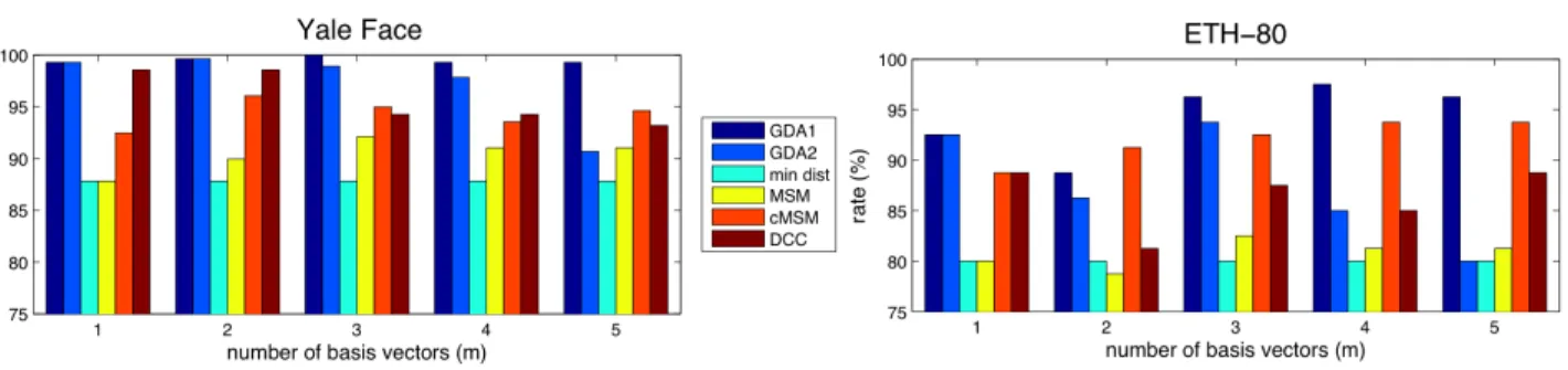
For each subject and each pose, we model the illumi-nation variations by a subspace of the sizem= 1, ...,5, spanned by the 1 to 5 largest eigenvectors from SVD. We evaluate the recognition rate of subjects with nine-fold cross validation, holding out one pose of all sub-jects from the training set and using it for test. The recognition rates are shown in Fig. 2. The GDA1

outperforms the other methods consistently. The

GDA2 also performs well for small m, but performs

worse as m becomes large. The rates of the others

also seem to decrease as m increases. An

interpreta-tion of the observainterpreta-tion is that the first few

eigenvec-tors from the data already have enough information and the smaller eigenvectors are spurious for discrim-inating the subjects.

6.3. Testing Pose-Invariance with ETH-80 Database

The ETH-80 (Leibe & Schiele, 2003) database con-sists of pictures of 8 object categories (‘apple’, ‘pear’, ‘tomato’, ‘cow’, ‘dog’, ‘horse’, ‘cup’, ‘car’). Each cat-egory has 10 objects that belong to the catcat-egory, and each object is recorded under 41 different poses.

Im-ages were resized to 32×32 pixels (D = 1024) and

normalized to have the same variance. For each cate-gory and each object, we model the pose variations by

a subspace of the size m = 1, ...,5, spanned by the 1

to 5 largest eigenvectors from SVD. We evaluate the classification rate of the categories with ten-fold cross validation, holding out one object instance of each cat-egory from the training set and using it for test. The recognition rates are also summarized in Fig. 2. The GDA1 also outperforms the other methods most of the time, but the cMSM performs better than GDA2

as m increases. The rates seem to peak around m =

4 and then decrease as m increases. This results is

consistent with the observation that the eigenvalues from this database decrease more gradually than the eigenvalues from the Yale face database.

7. Conclusion

In this paper we have proposed a Grassmann frame-work for problem in which data consist of subspaces. By using the Projection metric and the Binet-Cauchy metric, which are derived from the Grassmann ker-nels, we were able to apply kernel methods such as kernel LDA to subspace data. In addition to having theoretically sound grounds, the proposed method also outperformed state-of-the-art methods in two experi-ments with real data. As a future work, we are pur-suing a better understanding of probabilistic distribu-tions on the Grassmann manifold.

References

Absil, P., Mahony, R., & Sepulchre, R. (2004). Riemannian geometry of Grassmann manifolds with a view on algo-rithmic computation. Acta Appl. Math.,80, 199–220. Chang, J.-M., Beveridge, J. R., Draper, B. A., Kirby, M.,

Kley, H., & Peterson, C. (2006). Illumination face spaces are idiosyncratic. IPCV(pp. 390–396).

Chikuse, Y. (2003). Statistics on special manifolds, lecture notes in statistics, vol. 174. New York: Springer. Edelman, A., Arias, T. A., & Smith, S. T. (1999). The

Figure 2.Recognition rates of subjects from Yale face database (Left), and classification rates of categories in ETH-80 database (Right). The bars represent the rates of six algorithms (GDA1, GDA2, Min Dist, MSM, cMSM, DCC) evaluated form= 1, ....,5 wheremis the number of basis vectors for subspaces. The GDA1 achieves the best rates consistently, and the GDA2 also performs competitively for smallm.

geometry of algorithms with orthogonality constraints.

SIAM J. Matrix Anal. Appl.,20, 303–353.

Farag´o, A., Linder, T., & Lugosi, G. (1993). Fast nearest-neighbor search in dissimilarity spaces. IEEE Trans. Pattern Anal. Mach. Intell.,15, 957–962.

Fukui, K., & Yamaguchi, O. (2003). Face recognition using multi-viewpoint patterns for robot vision. Int. Symp. of Robotics Res.(pp. 192–201).

Fukunaga, K. (1990). Introduction to statistical pattern recognition (2nd ed.). San Diego, CA, USA: Academic Press Professional, Inc.

Georghiades, A. S., Belhumeur, P. N., & Kriegman, D. J. (2001). From few to many: Illumination cone models for face recognition under variable lighting and pose. IEEE Trans. Pattern Anal. Mach. Intell.,23, 643–660. Golub, G. H., & Loan, C. F. V. (1996). Matrix

compu-tations (3rd ed.). Baltimore, MD, USA: Johns Hopkins University Press.

Haasdonk, B. (2005). Feature space interpretation of svms with indefinite kernels. IEEE Trans. Pattern Anal. Mach. Intell.,27, 482–492.

Hein, M., Bousquet, O., & Sch¨olkopf, B. (2005). Maximal margin classification for metric spaces.J. Comput. Syst. Sci.,71, 333–359.

Kim, T.-K., Kittler, J., & Cipolla, R. (2007). Discrimi-native learning and recognition of image set classes us-ing canonical correlations. IEEE Trans. Pattern Anal. Mach. Intell.,29, 1005–1018.

Kondor, R. I., & Jebara, T. (2003). A kernel between sets of vectors.Proc. of the 20th Int. Conf. on Mach. Learn.

(pp. 361–368).

Leibe, B., & Schiele, B. (2003). Analyzing appearance and contour based methods for object categorization.CVPR,

02, 409.

Ong, C. S., Mary, X., Canu, S., & Smola, A. J. (2004). Learning with non-positive kernels. Proc. of 21st Int. Conf. on Mach. Learn.(p. 81). New York, NY, USA: ACM.

Pekalska, E., Paclik, P., & Duin, R. P. W. (2002). A gener-alized kernel approach to dissimilarity-based classifica-tion. J. Mach. Learn. Res.,2, 175–211.

Sakano, H.; Mukawa, N. (2000). Kernel mutual subspace method for robust facial image recognition.Proc. of Int. Conf. on Knowledge-Based Intell. Eng. Sys. and App. Tech.(pp. 245–248).

Schoenberg, I. J. (1938). Metric spaces and positive definite functions. Trans. Amer. Math. Soc.,44, 522–536. Sch¨olkopf, B., & Smola, A. J. (2001). Learning with

ker-nels: Support vector machines, regularization, optimiza-tion, and beyond. Cambridge, MA, USA: MIT Press. Shakhnarovich, G., John W. Fisher, I., & Darrell, T.

(2002). Face recognition from long-term observations.

Proc. of the 7th Euro. Conf. on Computer Vision (pp. 851–868). London, UK.

Turk, M., & Pentland, A. P. (1991). Eigenfaces for recog-nition. J. Cog. Neurosc.,3, 71–86.

Vishwanathan, S., & Smola, A. J. (2004). Binet-cauchy kernels. Proc. of Neural Info. Proc. Sys..

Wang, L., Wang, X., & Feng, J. (2006). Subspace distance analysis with application to adaptive bayesian algorithm for face recognition. Pattern Recogn.,39, 456–464.

Wolf, L., & Shashua, A. (2003). Learning over sets using kernel principal angles. J. Mach. Learn. Res., 4, 913– 931.

Wong, Y.-C. (1967). Differential geometry of Grassmann manifolds.Proc. of the Nat. Acad. of Sci., Vol. 57, 589– 594.

Yamaguchi, O., Fukui, K., & Maeda, K. (1998). Face recognition using temporal image sequence.Proc. of the 3rd. Int. Conf. on Face & Gesture Recognition(p. 318). Washington, DC, USA: IEEE Computer Society. Zhou, S. K., & Chellappa, R. (2006). From sample

similar-ity to ensemble similarsimilar-ity: Probabilistic distance mea-sures in reproducing kernel hilbert space. IEEE Trans. Pattern Anal. Mach. Intell.,28, 917–929.