Development and Assessment of the
1
SMAP Enhanced Passive Soil Moisture Product
2 3
Steven K. Chan, Rajat Bindlish, Peggy O’Neill, Thomas Jackson, Eni Njoku, 4
Scott Dunbar, Julian Chaubell, Jeffrey Piepmeier, Simon Yueh, Dara Entekhabi, 5
Andreas Colliander, Fan Chen, Michael H. Cosh, Todd Caldwell, Jeffrey Walker, 6
Aaron Berg, Heather McNairn, Marc Thibeault, José Martínez-Fernández, 7
Frederik Uldall, Mark Seyfried, David Bosch, Patrick Starks, Chandra Holifield Collins, 8
John Prueger, Rogier van der Velde, Jun Asanuma, Michael Palecki, Eric E. Small, 9
Marek Zreda, Jean-Christophe Calvet, Wade T. Crow, and Yann Kerr 10
11
S. K. Chan, J. Chaubell, S. Dunbar, A. Colliander, and S. Yueh are with the NASA
Jet Propulsion Laboratory, California Institute of Technology, Pasadena, CA 91109 USA (e-mail: [email protected]).
R. Bindlish, P. O’Neill, and J. Piepmeier are with the NASA Goddard Space Flight
Center, Greenbelt, MD 20771 USA.
T. Jackson, M. H. Cosh, and W. T. Crow are with the USDA ARS Hydrology and
Remote Sensing Laboratory, Beltsville, MD 20705 USA.
F. Chen is with Science Systems and Applications, Inc., Lanham, MD 20706 USA. D. Entekhabi is with the Massachusetts Institute of Technology, Cambridge, MA 02139
USA.
T. Caldwell is with the University of Texas, Austin, TX 78713 USA. J. Walker is with Monash University, Clayton, Vic. 3800, Australia.
A. Berg is with the University of Guelph, Guelph, ON N1G 2W1, Canada.
H. McNairn is with Agriculture and Agri-Food Canada, Ottawa, ON K1A OC6, Canada. M. Thibeault is with the Comisión Nacional de Actividades Espaciales (CONAE),
Buenos Aires, Argentina.
J. Martínez-Fernández is with the Instituto Hispano Luso de Investigaciones
Agrarias (CIALE), Universidad de Salamanca, 37185 Salamanca, Spain.
F. Uldall is with Center for Hydrology, Technical University of Denmark, Copenhagen,
Denmark.
M. Seyfried is with the USDA ARS Northwest Watershed Research Center, Boise, ID
83712 USA.
D. Bosch is with the USDA ARS Southeast Watershed Research Center, Tifton, GA
31793 USA.
P. Starks is with the USDA ARS Grazinglands Research Laboratory, El Reno, OK 73036
USA.
C. Holifield Collins is with the USDA ARS Southwest Watershed Research Center,
Tucson, AZ 85719 USA.
J. Prueger is with the USDA ARS National Laboratory for Agriculture and the
Environment, Ames, IA 50011 USA.
R. van der Velde is with the University of Twente, Enschede, Netherlands. J. Asanuma is with the University of Tsukuba, Tsukuba, Japan.
M. Palecki is with NOAA National Climatic Data Center, Asheville, NC 28801 USA. E. E. Small is with the University of Colorado, Boulder, CO 80309 USA.
J. Calvet is with CNRM-GAME, UMR 3589 (Météo-France, CNRS), Toulouse, France. Y. Kerr is with CESBIO-CNES, Toulouse, France.
E. Njoku, retired, was with the NASA Jet Propulsion Laboratory, California Institute of
Technology, Pasadena, CA 91109 USA. 12
Abstract
13 14
Launched in January 2015, the National Aeronautics and Space Administration (NASA) 15
Soil Moisture Active Passive (SMAP) observatory was designed to provide frequent global 16
mapping of high-resolution soil moisture and freeze-thaw state every two to three days 17
using a radar and a radiometer operating at L-band frequencies. Despite a hardware 18
mishap that rendered the radar inoperable shortly after launch, the radiometer continues 19
to operate nominally, returning more than two years of science data that have helped to 20
improve existing hydrological applications and foster new ones. 21
22
Beginning in late 2016 the SMAP project launched a suite of new data products with the 23
objective of recovering some high-resolution observation capability loss resulting from 24
the radar malfunction. Among these new data products are the SMAP Enhanced Passive 25
Soil Moisture Product that was released in December 2016, followed by the 26
SMAP/Sentinel-1 Active-Passive Soil Moisture Product in April 2017. 27
28
This article covers the development and assessment of the SMAP Level 2 Enhanced 29
Passive Soil Moisture Product (L2_SM_P_E). The product distinguishes itself from the 30
retrieval is posted on a 9 km grid instead of a 36 km grid. This is made possible by first 32
applying the Backus-Gilbert optimal interpolation technique to the antenna temperature 33
(TA) data in the original SMAP Level 1B Brightness Temperature Product to take
34
advantage of the overlapped radiometer footprints on orbit. The resulting interpolated 35
TA data then go through various correction/calibration procedures to become the SMAP
36
Level 1C Enhanced Brightness Temperature Product (L1C_TB_E). The L1C_TB_E 37
product, posted on a 9 km grid, is then used as the primary input to the current 38
operational SMAP baseline soil moisture retrieval algorithm to produce L2_SM_P_E as 39
the final output. Images of the new product reveal enhanced visual features that are not 40
apparent in the standard product. Based on in situ data from core validation sites and 41
sparse networks representing different seasons and biomes all over the world, 42
comparisons between L2_SM_P_E and in situ data were performed for the duration of 43
April 1, 2015 – October 30, 2016. It was found that the performance of the enhanced 9 44
km L2_SM_P_E is equivalent to that of the standard 36 km L2_SM_P, attaining a 45
retrieval uncertainty below 0.040 m3/m3 unbiased root-mean-square error (ubRMSE)
46
and a correlation coefficient above 0.800. This assessment also affirmed that the Single 47
Channel Algorithm using the V-polarized TB channel (SCA-V) delivered the best retrieval
48
performance among the various algorithms implemented for L2_SM_P_E, a result 49
similar to a previous assessment for L2_SM_P. 50
51
Keywords: SMAP; enhanced; soil moisture; passive; retrieval; validation; assessment 52
53
1. Introduction
54 55
The synergy of active (radar) and passive (radiometer) technologies at L-band microwave 56
frequencies in the National Aeronautics and Space Administration (NASA) Soil Moisture 57
Active Passive (SMAP) mission provides a unique remote sensing opportunity to measure 58
soil moisture with unprecedented accuracy, resolution, and coverage (Entekhabi, et al., 59
2014). Driven by the needs in hydroclimatological and hydrometeorological applications, 60
the SMAP observatory was designed to meet a soil moisture retrieval accuracy 61
requirement of 0.040 m3/m3 unbiased root-mean-square error (ubRMSE) or better at a
62
spatial resolution of 10 km over non-frozen land surfaces that are free of excessive snow, 63
ice, and dense vegetation coverage (Entekhabi, et al., 2014). 64
In July 2015, SMAP’s radar stopped working due to an irrecoverable hardware 65
failure, leaving the radiometer as the only operational instrument onboard the 66
observatory. Since the beginning of science data acquisition in April 2015, the radiometer 67
has been collecting L-band (1.41 GHz) brightness temperature (TB) data at a spatial
68
resolution of 36 km, providing global coverage every two to three days. The relatively 69
high fidelity of the data provided by the radiometer’s radio-frequency-interference (RFI) 70
mitigation hardware (Piepmeier, et al., 2015; Mohammed, et al., 2016), along with the 71
observatory’s full 360-degree view that offers both fore- and aft-looking observations, 72
presents unique advantages for SMAP data to advance established hydrological 73
applications (Koster, et al., 2016) and foster new ones (Yueh, et al., 2016). 74
75
Despite the loss of the radar, SMAP is committed to providing high-resolution 76
observations to the extent that is possible. This initiative of acquiring high-resolution 77
information proceeds in two distinct approaches. The first approach involves combining 78
observations from other satellites in space to produce an operational soil moisture 80
product similar to the now discontinued SMAP Level 2 Active-Passive Soil Moisture 81
Product (L2_SM_AP). To attain this objective, the high-resolution synthetic aperture 82
radar (SAR) data from the European Space Agency (ESA) Sentinel-1 C-band radar 83
constellation (Torres, et al., 2012) represent the most optimal candidate data source that 84
would provide partial fulfillment of the original science benefits of L2_SM_AP. Although 85
there are technical challenges due to data latency, global coverage, revisit frequency, and 86
retrieval performance from such a combined L/C-band SMAP/Sentinel-1 soil moisture 87
product, these challenges are expected to be mitigated over time under the close 88
collaboration between the two mission teams. The resulting SMAP/Sentinel-1 Level 2 89
Active-Passive Product (L2_SM_SP) will be available to the public in April 2017. 90
The second approach is based on the application of the Backus-Gilbert (BG) optimal 91
interpolation technique (Poe, 1990; Stogryn, 1978) to the antenna temperature (TA)
92
measurements in the original SMAP Level 1B Brightness Temperature Product (L1B_TB) 93
(Piepmeier, et al., 2015a; 2015b). The resulting interpolated TA data then go through the
94
standard correction/calibration procedures to produce the SMAP Level 1C Enhanced 95
Brightness Temperature Product (L1C_TB_E) on a set of 9 km grids (Chaubell, et al., 96
2016). The objective of the BG interpolation as implemented by SMAP is to achieve 97
optimal brightness temperature (TB) estimates at arbitrary locations as if original
98
observations were available at the same locations (Poe, 1990). This estimation is achieved 99
by linearly combining optimally weighted radiometric measurements overlapped in both 100
along- and across-scan directions. The BG procedure is an improvement over what the 101
current SMAP Level 1C Brightness Temperature Product (L1C_TB) (Chan et al., 2014, 102
2015) offers, in that it makes explicit use of antenna pattern information and finer grid 103
posting to more fully capture the high spatial frequency information in the original 104
oversampled radiometer measurements in the along-scan direction (Chaubell, 2016). It 105
is important to note that this recovery of high spatial frequency information as 106
implemented in this approach primarily comes from interpolation instead of beam 107
sharpening. As such, the native resolution of the interpolated data remains to be about 108
the same as the spatial extent projected on earth surface by the 3-dB beamwidth of the 109
radiometer. For SMAP, this spatial extent is roughly an ellipse with 36 km as its minor 110
axis and 47 km as its major axis (Entekhabi, et al., 2014). As the SMAP project adopted 111
the square root of footprint area as the definition of native resolution of the radiometer, 112
the corresponding native resolution is estimated to be (π/4 × 36 × 47)1/2 ~ 36 km. The
113
resulting L1C_TB_E data are posted on the EASE Grid 2.0 projection (Brodzik, et al., 114
2012, 2014) at a grid spacing of 9 km, even though the data actually exhibit a native 115
resolution of ~36 km. The L1C_TB_E product is then used as the primary input in 116
subsequent passive geophysical inversion to produce the SMAP Level 2 Enhanced Passive 117
Soil Moisture Product (L2_SM_P_E) (O’Neill, et al., 2016), which is the focus of this 118
paper. 119
The retrieval performance of L2_SM_P_E was assessed and reported in this paper 120
using more than 1.5 years (April 1, 2015 – October 30, 2016) of in situ data from core 121
validation sites (CVSs) and sparse networks representing different seasons and biomes 122
all over the world. The assessment findings presented in this paper represent a significant 123
extension of the work reported in (Chan, et al., 2016). Additional metric statistics from 124
this assessment can be found in a separate report that covers the standard and enhanced 125
passive soil moisture products (Jackson, et al., 2016). 126
2. Product Development
128 129
The SMAP observatory was to present a unique opportunity to demonstrate the synergy 130
of radar and radiometer observations at L-band frequencies in the remote sensing of soil 131
moisture and freeze/thaw state detection from space. Unfortunately, this demonstration 132
was shortened due to a hardware failure that eventually halted the operation of the radar 133
after about three months of operation. While the loss necessarily ended the operational 134
production of several key soil moisture and freeze/thaw data products that rely on the 135
high-resolution radar data, it also spurred the development of several new data products 136
designed to recover as much high-resolution information as possible. 137
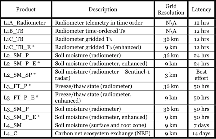
Table 1 shows a list of SMAP data products that are or will be in routine operational 138
production. There are two main groups of data products in the table: enhanced products 139
(with asterisks) and standard products (without asterisks). The standard products are 140
those that have been available since the beginning of the mission and will continue to be 141
available operationally. The enhanced products, on the other hand, represent new 142
products developed after the loss of the SMAP radar; these products contain enhanced 143
information derived from the existing radiometer observations or new external data from 144
other satellites. For example, the L2_SM_SP product is a product derived from the 145
SMAP’s L-band radiometer observations and the Sentinel-1’s C-band SAR data (Torres, 146
et al., 2012). This product will be available to the public in April 2017. Other enhanced 147
products (L1C_TB_E L2_SM_P_E, L3_SM_P_E, L3_FT_P, and L3_FT_P_E) are 148
derived primarily from the existing radiometer observations. These products have been 149
available to the public since December 2016. Of these radiometer-only enhanced 150
products, L1C_TB_E and L2_SM_P_E will be covered in greater detail in Sections 2.1 151
and 2.2, respectively. A more comprehensive list of SMAP data products, including those 152
that have been discontinued, can be found in Entekhabi, et al., 2014. 153
154
Table 1: SMAP data products that are or will be in routine operational production. 155
156
Product Description Resolution Grid Latency
L1A_Radiometer Radiometer telemetry in time order N\A 12 hrs
L1B_TB Radiometer time-ordered TB N\A 12 hrs
L1C_TB Radiometer gridded TB 36 km 12 hrs
L1C_TB_E * Radiometer gridded TB (enhanced) 9 km 12 hrs
L2_SM_P Soil moisture (radiometer) 36 km 24 hrs
L2_SM_P_E * Soil moisture (radiometer, enhanced) 9 km 24 hrs L2_SM_SP * Soil moisture (radiometer + Sentinel-1
radar) 3 km
Best effort L3_FT_P * Freeze/thaw state (radiometer) 36 km 50 hrs L3_FT_P_E * Freeze/thaw state (radiometer,
enhanced) 9 km 50 hrs
L3_SM_P Soil moisture (radiometer) 36 km 50 hrs
L3_SM_P_E * Soil moisture (radiometer, enhanced) 9 km 50 hrs L4_SM Soil moisture (surface and root zone) 9 km 7 days L4_C Carbon net ecosystem exchange (NEE) 9 km 14 days 157
2.1 Enhanced Brightness Temperature
158 159
Passive soil moisture inversion begins with TB observations. For SMAP, to more fully
160
capture the information in the oversampled along-scan TB observations, the BG
161
interpolation technique is applied to the TA measurements in the standard L1B_TB
162
product in the SMAP’s Science Data System (SDS). The resulting interpolated TA data
163
then go through the standard correction/calibration procedures to produce the 164
L1C_TB_E product. The BG implementation in SDS follows the same approach described 165
in (Poe, 1990) that makes use of antenna pattern information to produce TB estimates at
166
arbitrary sampling locations. The procedure is considered optimal in the sense that its 167
estimates are supposed to minimize differences relative to what would have been 168
measured had the instrument actually sampled at the same locations. For immediate 169
application to soil moisture and freeze/thaw state detection in SMAP product production, 170
the TB values in L1C_TB_E are posted on the 9 km EASE Grid 2.0 in global cylindrical
171
projection, north polar projection, and south polar projection. Only the TB values on
172
global projection are used in passive soil moisture inversion. A more in-depth account of 173
the theory behind the BG implementation in SDS can be found in the Algorithm 174
Theoretical Basis Document (ATBD) (Chaubell, 2016) and Assessment Report (Piepmeier, 175
et al., 2016) that accompany the product. Besides the ATBD, the Product Specification 176
Document (PSD) (Chan and Dunbar, 2016) is also available on the NASA Distributed 177
Active Archive Center (DAAC) at the National Snow and Ice Data Center (NSIDC) for 178
informed applications of the product. 179
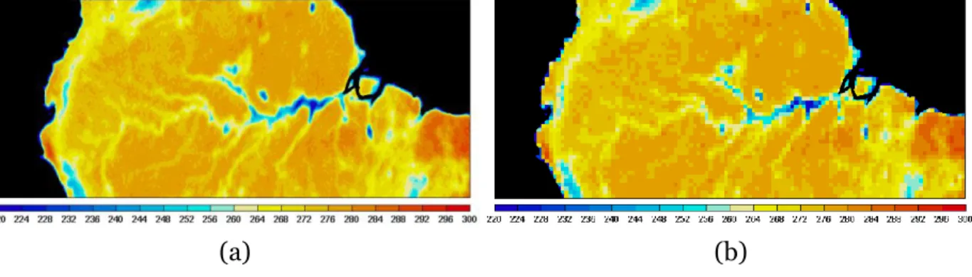
Figure 1 illustrates the horizontally polarized TB observations obtained by SMAP
180
between December 15–17, 2016 over the Amazon basin before and after the application 181
of BG interpolation. This area was selected because the domain features well-defined 182
river tracks punctuated with highly visible fine-scale spatial structures in the midst of a 183
relatively homogeneous background. It is clear from the comparison that the enhanced 184
L1C_TB_E (Fig. 1a) is able to reveal spatial features that are concealed or not immediately 185
obvious in the standard L1C_TB (Fig. 1b). Overall, the L1C_TB_E image also presents a 186
less pixelated representation of the original TB data due to its posting on a finer grid.
187 188
(a) (b) 189
Figure 1: SMAP horizontally polarized TB observations obtained between
190
December 15–17, 2016 over the Amazon basin: (a) L1C_TB_E and (b) 191
L1C_TB.. 192
193
It is important to note that the improvement in L1C_TB_E image quality primarily 194
comes from an interpolation scheme that is an improvement over what is used in the 195
standard product. The interpolation in L1C_TB_E more fully captures the information 196
from the oversampled along-scan TB observations without degrading the native resolution
197
of the radiometer. This aspect regarding the native resolution of the product had been 198
extensively vetted during product development in a series of matchup analyses using the 199
original time-ordered L1B_TB TB data points as the benchmark data set. The matchup
200
analyses began with collocating pairs of L1C_TB_E TB data points and L1B_TB TB data
201
points that are within a small distance from each other (< 2 km, which is less than the 202
L1B_TB geolocation error allocation (Piepmeier, et al., 2015)). The collocated pairs were 203
stored separately for ascending and descending passes, and also for fore- and aft-looking 204
observations to minimize azimuthal mismatch. The collocated data pairs from these four 205
matchup collections (i.e., ascending/fore, ascending/aft, descending/fore, and 206
descending/aft) were then averaged over all orbits between April 1, 2015 and October 30, 207
2016 for all grid cells in the 9 km global EASE Grid 2.0 projection. Even though the 208
L1C_TB_E data values are posted on a grid, they are expected to be almost identical to 209
the corresponding L1B_TB data values at the same grid locations due to the close 210
proximity between the two. 211
Given their impulse-like radiometric responses, small and isolated islands in the 212
ocean provide ideal locations to compare the native resolution of L1C_TB_E against the 213
known native resolution of L1B_TB using the collocated data pairs described above. This 214
approach of using discrete islands to evaluate data native resolution has been extensively 215
explored in the study of resolution-enhanced scatterometer data (Bradley and Long, 216
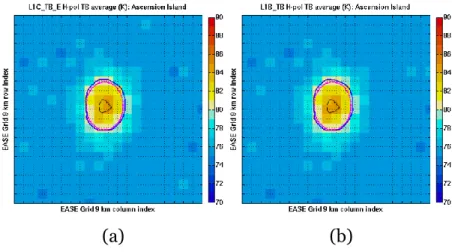
2014). Figure 2 describes one such comparison performed over Ascension Island 217
(7.93ºS,14.417ºW) located approximately midway between the coasts of Brazil and Africa 218
in the South Atlantic Ocean. The island is about 10.07 km across and exhibits near 219
azimuthal symmetry. Based on the peak values of L1C_TB_E (Fig. 2a) and L1B_TB (Fig. 220
2b), contours that correspond to one half of their respective peak values were estimated 221
around the island. These 3-dB contours, which are indicative of the native resolution of 222
the underlying data, are depicted by the blue lines in the figures. The magenta lines in 223
both figures are identical; they correspond to the 3-dB contours estimated based on the 224
geometry of the projected instantaneous field-of-view (IFOV) of the radiometer. The 225
good agreement in 3-dB contour estimation between radiometric estimation (blue lines) 226
and geometric calculation (magenta lines) confirms that small and isolated islands such 227
as Ascension Island can indeed provide a good approximation for the impulse response 228
from a point target. 229
(a) (b)
231
Figure 2: Comparison of data native resolution between L1C_TB_E and 232
L1B_TB based on radiometric estimation (blue lines) and geometric 233
calculation (magenta lines): (a) L1C_TB_E and (b) L1B_TB. 234
235
The comparison shows that after BG interpolation the 3-dB contour of L1C_TB_E in Fig. 236
2a is about the same size as the 3-dB contour of L1B_TB in Fig. 2b, confirming that the 237
enhanced product preserves the native resolution and noise characteristics of the 238
radiometer while providing an optimal interpolation approach that more fully utilizes the 239
oversampled along-scan TB measurements in the original data. Further analyses on other
240
small and isolated islands yielded the same conclusions. The TB signatures between
241
L1C_TB_E in Fig. 2a and L1B_TB in Fig. 2b are similar, suggesting that the current BG 242
implementation indeed preserves the original data at locations where L1B_TB 243
measurements are available. 244
245
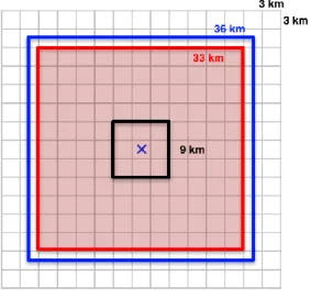
The native resolution of L1C_TB_E determines the spatial scale by which the 246
subsequent L2_SM_P_E should be developed and assessed. It was found that when 3 247
km ancillary data (Table 2) are aggregated as inputs to L2_SM_P_E that is posted on a 9 248
km grid, a contributing domain of 33 km × 33 km (Section 3.1) is necessary to cover a 249
spatial extent similar to the native resolution of the radiometer, as shown in Fig. 3. This 250
contributing domain was thus adopted in L2_SM_P_E product development (Section 2.2) 251
and assessment (Section 3). 252
253
254 255
Figure 3: With L2_SM_P_E (black) and ancillary data (gray) posted at 9 256
km and 3 km, respectively, a contributing domain of 33 km × 33 km (red) is 257
necessary to cover a spatial extent similar to the native resolution (blue) of 258
the radiometer. 259
260
It is anticipated that future SDS BG implementations could improve the current 261
L1C_TB_E native resolution beyond the radiometer IFOV. Such an improvement will 262
require an alternate contributing domain that approximates the new native resolution in 263
revised L2_SM_P_E development and assessment. 264
2.2 Enhanced Passive Soil Moisture
266 267
The development of L2_SM_P_E follows a close parallel with that of L2_SM_P (Chan, et 268
al., 2016; O’Neill, et al., 2015). Both products share the same basic implementation 269
elements, ranging from processing flow, ancillary data, and retrieval algorithms. Figure 270
4 illustrates the flow of the L2_SM_P_E processor. The fore- and aft-look TB
271
observations in L1C_TB_E are first combined to provide the primary input to the 272
processor. Static and dynamic ancillary data (Table 2) preprocessed on finer grid 273
resolutions are then brought into the processing to evaluate the feasibility of the retrieval. 274
If retrieval is deemed feasible at a given location, the processor will further evaluate the 275
quality of the retrieval. When surface conditions favorable to soil moisture retrieval are 276
identified, corrections for surface roughness, effective soil temperature, vegetation water 277
content, and radiometric contribution by water bodies are applied. The baseline soil 278
moisture retrieval algorithm is then invoked with TB observations and ancillary data as
279
inputs to produce L2_SM_P_E on the same 9 km EASE Grid 2.0 global projection as the 280
input L1C_TB_E. A full description of L2_SM_P_E data contents can be found in the 281
Product Specification Document (Chan, 2016). 282
284 285
Figure 4: L2_SM_P_E processor design. The processor uses L1C_TB_E 286
and ancillary data as primary inputs to perform geophysical inversion under 287
favorable surface conditions. The resulting L2_SM_P_E soil moisture 288
estimates are posted on the same 9 km EASE Grid 2.0 global projection as 289
the input L1C_TB_E. 290
291
Table 2: Ancillary data used in L2_SM_P_E and L2_SM_P processing. 292
293
Ancillary Data Resolution Grid Resolution Time Primary Data Source
Water fraction 3 km Static MODIS MOD44W (Chan, 2013)
Urban fraction 3 km Static Global Rural Urban Mapping Project (GRUMP) (Das, 2013) DEM slope variability 3 km Static USGS GMTED 2010 (Podest and Crow, 2013) Soil texture 3 km Static FAO Harmonized World Soil Database (HWSD) (Das, 2013)
Land cover 3 km Static MODIS MCD12Q1 (V051) (Kim, 2013)
NDVI 3 km 2000–2013 MODIS MOD13A2 (V005) (Chan, 2013)
Snow fraction 9 km Daily NOAA IMS (Kim, 2011)
Soil temperatures 9 km 1 hourly GMAO GEOS-5 (SMAP, 2015)
Precipitation 9 km 3 hourly GMAO GEOS-5 (Dunbar, 2013)
294
Because of its improved representation of the original TB data, the enhanced 9 km
295
L1C_TB_E product contains additional spatial information that is not available in the 296
standard 36 km L1C_TB product, as exemplified in a series of spectral analysis on small 297
and isolated islands in the ocean (Piepmeier, et al., 2016). When used as the primary 298
input to the enhanced 9 km L2_SM_P_E product, the additional spatial information 299
results in enhanced visual details that are also not available in the standard 36 km 300
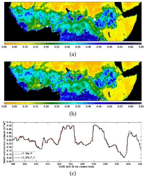
L2_SM_P product. Figure 5 contrasts the amount of visual details between L2_SM_P_E 301
(Fig. 5a) and L2_SM_P (Fig. 5b) over the vegetation transition region in Africa. After the 302
application of the baseline soil moisture retrieval algorithm to L1C_TB_E, the resulting 303
L2_SM_P_E on a 9 km grid shows a higher acuity compared with L2_SM_P on a 36 km 304
grid. This enhancement in spatial details is further illustrated in Fig. 5c in which the soil 305
moisture variability of L2_SM_P_E (black line) and L2_SM_P (red line) along the two 306
identical magenta lines in Figs. 5a and 5b is plotted together. The enhanced and standard 307
products mostly track each other and follow the same macroscopic spatial patterns along 308
the transect without obvious bias or unusual artifacts. In addition, there are locations 309
(e.g. between column indices 512 and 515 in Fig. 5c) where L2_SM_P_E appears to 310
capture fine-scale soil moisture variability that is not available in L2_SM_P. It is 311
important to note that throughout the L2_SM_P_E processing, no new or additional 312
ancillary datasets other than those listed in Table 2 are brought into the processing. The 313
observed enhanced spatial details revealed in L2_SM_P_E are thus primarily contributed 314
by the additional spatial information in L1C_TB_E. 315
316
(a)
(b)
(c) 317
Figure 5: Soil moisture estimates in m3/m3 of (a) L2_SM_P_E, (b)
318
L2_SM_P, and (c) L2_SM_P_E and L2_SM_P along the two identical 319
magenta lines in (a) and (b). 320
321
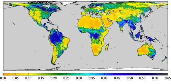
On a global scale, the enhanced product exhibits the expected geographical 322
patterns of soil moisture. Figure 6 represents a three-day composite of 6:00 am 323
descending L2_SM_P_E between September 20–22, 2016. The expected patterns of 324
L2_SM_P_E soil moisture estimates in m3/m3 qualitatively affirm the soundness of the
325
underlying baseline soil moisture retrieval algorithm. Section 3 covers the quantitative 326
aspect of the assessment for the product based on comparison with in situ soil moisture 327
observations. 328
329
Figure 6: Global pattern of soil moisture estimates in m3/m3 of
330
L2_SM_P_E based on 6:00 am descending TB data between September
331 20–22, 2016. 332 333 3. Product Assessment 334 335
The retrieval accuracy of L2_SM_P_E was assessed using the same validation 336
methodologies for L2_SM_P as reported in (Chan, et al., 2016; Colliander, et al., 2017). 337
Nineteen months (April 2015 through October 2016) of in situ soil moisture observations 338
were used as ground truth to evaluate the performance of the product. Much deliberation 339
on criteria that would ensure data quality, sensor maintenance and calibration stability, 341
biome diversity, and geographical representativeness. The in situ data consist of scaled 342
aggregations of in situ soil moisture observations at a nominal soil depth of 5 cm to mimic 343
L2_SM_P_E soil moisture estimates at satellite footprint scale. All in situ data were 344
provided through a collaboration with domestic and international calibration/validation 345
(cal/val) partners who operate and maintain calibrated soil moisture measuring sensors 346
in their core validation sites (CVSs) (Colliander, et al., 2017; Smith, et al., 2012; Yee, et al., 347
2016) or sparse networks (Chen, et al., 2017). 348
Agreement between the L2_SM_P_E soil moisture estimates and in situ data over 349
space and time are reported in four metrics: 1) unbiased root-mean-square error 350
(ubRMSE), 2) bias (defined as L2_SM_P_E minus in situ data), 3) root-mean-square 351
error (RMSE), and 4) correlation (R). Together, these metrics provide a more complete 352
description of product performance than any one alone (Entekhabi, et al., 2010). Among 353
these metrics, however, the ubRMSE computed from in situ data comparison at CVSs is 354
adopted for reporting the product accuracy of L2_SM_P_E, with an accuracy target of 355
0.040 m3/m3 that mimics the SMAP Level 1 mission accuracy requirement for the now
356
discontinued SMAP Level 2 Active-Passive Soil Moisture Product (L2_SM_AP) 357
(Entekhabi, et al., 2010). 358
In addition to L2_SM_P_E, the retrieval performance of L2_SM_P and soil 359
moisture estimates by the Soil Moisture and Ocean Salinity (SMOS) mission (Kerr, et al., 360
2016) was also provided for comparison. In this assessment, both L2_SM_P_E and 361
L2_SM_P were based on version R13080 of the standard L1B_TB product, whereas 362
versions 551 and 621 of the SMOS Level 2 soil moisture product were used for April 1 - 363
May 4, 2015 and May 5, 2015 - October 31, 2016, respectively. For both SMAP and SMOS 364
soil moisture data products, only those soil moisture estimates whose retrieval quality 365
fields indicated good retrieval quality were considered and used in metric calculations. 366
The selection involved data of recommended quality as indicated in the retrieval quality 367
flag for the SMAP product, and data with unset FL_NO_PROD and retrieval DQX < 0.07 368
for the SMOS product. 369
Compared with L2_SM_P, L2_SM_P_E is expected to exhibit a higher serial 370
correlation of retrieval uncertainty over space. This higher correlation is a direct result of 371
the original L1B_TB interpolated on a finer grid posting (9 km) for L2_SM_P_E than the 372
original grid posting (36 km) for L2_SM_P. A full investigation into the spatial 373
correlation characteristics between the standard and enhanced products is beyond the 374
scope of this assessment. 375
376
3.1 Core Validation Sites
377 378
Although in general limited in quantity and spatial extent, CVSs provide in situ soil 379
moisture observations that, when properly scaled and aggregated, provide a 380
representative spatial average of soil moisture at the spatial scale of L2_SM_P_E (Section 381
2.1). In this assessment, CVS in situ data between April 2015 and October 2016 from a 382
total of 15 global sites were aggregated over a contributing domain of 33 km × 33 km (Fig. 383
3 in Section 2.1) around the sites. This area was chosen so that on a 9 km grid the resulting 384
aggregated ancillary data cover a spatial extent similar to the native resolution of the 385
radiometer (Section 2.1). Within this domain, CVS in situ data were scaled and 386
aggregated to provide the reference soil moisture for comparison. L2_SM_P_E soil 387
then extracted to match up in space and time with the corresponding CVS in situ data. 389
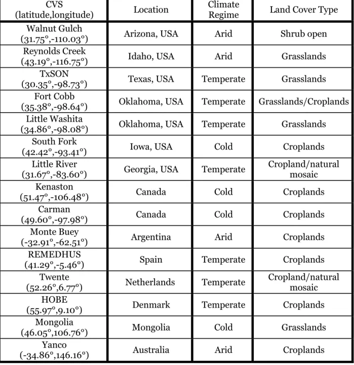
Table 3 lists the CVSs used in the assessment, along with their geographical locations, 390
climate regimes, and land cover types. 391
392
Table 3: CVSs used in L2_SM_P_E assessment. 393
394
CVS
(latitude,longitude) Location Climate Regime Land Cover Type Walnut Gulch
(31.75°,-110.03°) Arizona, USA Arid Shrub open
Reynolds Creek
(43.19°,-116.75°) Idaho, USA Arid Grasslands
TxSON
(30.35°,-98.73°) Texas, USA Temperate Grasslands Fort Cobb
(35.38°,-98.64°) Oklahoma, USA Temperate Grasslands/Croplands Little Washita
(34.86°,-98.08°) Oklahoma, USA Temperate Grasslands South Fork
(42.42°,-93.41°) Iowa, USA Cold Croplands
Little River
(31.67°,-83.60°) Georgia, USA Temperate Cropland/natural mosaic Kenaston
(51.47°,-106.48°) Canada Cold Croplands
Carman
(49.60°,-97.98°) Canada Cold Croplands
Monte Buey
(-32.91°,-62.51°) Argentina Arid Croplands
REMEDHUS
(41.29°,-5.46°) Spain Temperate Croplands
Twente
(52.26°,6.77°) Netherlands Temperate
Cropland/natural mosaic HOBE
(55.97°,9.10°) Denmark Temperate Croplands
Mongolia
(46.05°,106.76°) Mongolia Cold Grasslands
Yanco
395
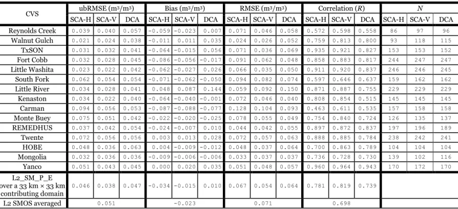
Tables 4 and 5 summarize the performance metrics that characterize the retrieval 396
performance of the 6:00 am descending and 6:00 pm ascending L2_SM_P_E soil 397
moisture estimates at CVSs for the baseline and two other candidate soil moisture 398
retrieval algorithms (SCA-H: Single Channel Algorithm using the H-polarized TB channel
399
and DCA: Dual Channel Algorithm) (O’Neill, et al., 2015). Compared with the other two 400
candidate algorithms, the SCA-V baseline algorithm was able to deliver the best overall 401
retrieval performance, achieving an average ubRMSE of 0.038 m3/m3 (6:00 am
402
descending) and 0.039 m3/m3 (6:00 pm ascending) as well as correlation of 0.819 (6:00
403
am descending) and 0.814 (6:00 pm ascending). In addition, the 6:00 am estimates were 404
shown to be in closer agreement with the CVS in situ soil moisture observations than the 405
6:00 pm estimates. This asymmetry in performance is particularly noticeable from the 406
bias metric: -0.015 m3/m3 (6:00 am descending) vs. -0.027 m3/m3 (6:00 pm ascending).
407
The overall dry bias is likely due to the inadequate depth correction for the GMAO 408
ancillary surface temperatures (Table 2) used to account for the difference between the 409
model soil depth and the actual physical sensing soil depth at L-band frequency, although 410
other algorithm assumptions which are more likely to be true at 6:00 am than at 6:00 pm 411
could also contribute to the overall asymmetry in performance. Further refinements in 412
the correction procedure for the effective soil temperature described in (Chan, et al., 2016; 413
Choudhury et al., 1982) are expected to improve the observed biases and reduce the performance gap between the 6:00 am 414
and 6:00 pm soil moisture estimates in future updates of the product. Both L2_SM_P_E and L2_SM_P displayed similar 415
retrieval performance when assessed at effectively the same spatial scale. 416
417
Table 4: Comparison between the 6:00 am descending L2_SM_P_E soil moisture estimates and CVS in situ 418
soil moisture observations between April 2015 and October 2016. 419
420
CVS ubRMSE (m
3/m3) Bias (m3/m3) RMSE (m3/m3) Correlation (R) N
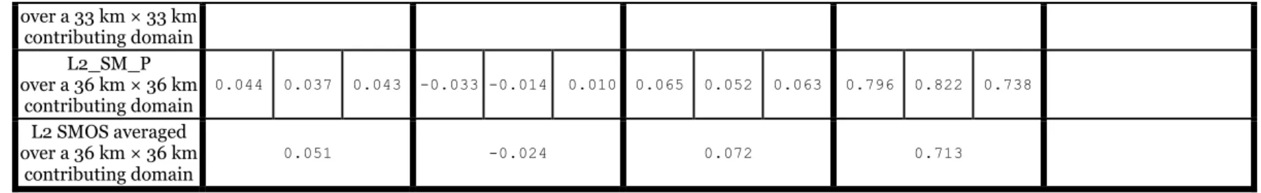
SCA-H SCA-V DCA SCA-H SCA-V DCA SCA-H SCA-V DCA SCA-H SCA-V DCA SCA-H SCA-V DCA Reynolds Creek 0.039 0.040 0.057 -0.059 -0.023 0.007 0.071 0.046 0.058 0.572 0.598 0.558 86 97 96 Walnut Gulch 0.021 0.024 0.038 -0.011 0.011 0.035 0.024 0.026 0.052 0.759 0.813 0.800 93 118 115 TxSON 0.031 0.032 0.041 -0.064 -0.015 0.056 0.071 0.036 0.069 0.935 0.921 0.827 153 153 152 Fort Cobb 0.032 0.028 0.045 -0.086 -0.056 -0.017 0.091 0.062 0.048 0.858 0.883 0.817 244 247 247 Little Washita 0.023 0.022 0.042 -0.062 -0.027 0.026 0.066 0.035 0.050 0.911 0.920 0.837 246 246 245 South Fork 0.062 0.054 0.054 -0.071 -0.062 -0.050 0.094 0.082 0.074 0.597 0.646 0.637 159 162 162 Little River 0.034 0.028 0.041 0.048 0.087 0.144 0.059 0.092 0.150 0.871 0.887 0.755 229 229 229 Kenaston 0.034 0.022 0.040 -0.064 -0.040 -0.001 0.072 0.046 0.040 0.808 0.854 0.515 145 145 145 Carman 0.094 0.056 0.053 -0.087 -0.088 -0.077 0.128 0.104 0.093 0.463 0.611 0.535 157 158 158 Monte Buey 0.075 0.051 0.042 -0.022 -0.020 -0.025 0.078 0.055 0.049 0.754 0.840 0.724 126 135 137 REMEDHUS 0.037 0.042 0.054 -0.024 -0.007 0.010 0.044 0.042 0.055 0.897 0.872 0.837 197 196 189 Twente 0.072 0.056 0.056 0.003 0.013 0.028 0.072 0.057 0.063 0.888 0.885 0.784 238 242 241 HOBE 0.048 0.036 0.063 0.004 -0.009 -0.012 0.048 0.037 0.064 0.700 0.863 0.789 104 104 104 Mongolia 0.032 0.036 0.036 -0.009 -0.006 -0.006 0.033 0.037 0.037 0.736 0.728 0.730 139 102 116 Yanco 0.051 0.043 0.045 0.000 0.020 0.035 0.051 0.048 0.057 0.960 0.964 0.943 170 172 170 L2_SM_P_E over a 33 km × 33 km contributing domain 0.046 0.038 0.047 -0.034 -0.015 0.010 0.067 0.054 0.064 0.781 0.819 0.739 L2 SMOS averaged 0.051 -0.023 0.071 0.698
over a 33 km × 33 km contributing domain L2_SM_P over a 36 km × 36 km contributing domain 0.044 0.037 0.043 -0.033 -0.014 0.010 0.065 0.052 0.063 0.796 0.822 0.738 L2 SMOS averaged over a 36 km × 36 km contributing domain 0.051 -0.024 0.072 0.713 421
Table 5: Comparison between the 6:00 pm ascending L2_SM_P_E soil moisture estimates and CVS in situ 422
soil moisture observations between April 2015 and October 2016. 423
424
CVS ubRMSE (m3/m3) Bias (m3/m3) RMSE (m3/m3) Correlation (R) N
SCA-H SCA-V DCA SCA-H SCA-V DCA SCA-H SCA-V DCA SCA-H SCA-V DCA SCA-H SCA-V DCA Reynolds Creek 0.046 0.042 0.060 -0.075 -0.042 -0.005 0.088 0.059 0.060 0.452 0.651 0.630 79 106 96 Walnut Gulch 0.027 0.029 0.042 -0.031 -0.019 -0.000 0.041 0.034 0.042 0.622 0.676 0.631 102 165 141 TxSON 0.028 0.028 0.033 -0.058 -0.018 0.031 0.065 0.034 0.045 0.930 0.929 0.893 178 178 178 Fort Cobb 0.039 0.035 0.046 -0.087 -0.069 -0.046 0.096 0.077 0.065 0.811 0.846 0.778 240 251 245 Little Washita 0.027 0.026 0.042 -0.057 -0.032 0.000 0.063 0.041 0.042 0.909 0.910 0.835 259 259 258 South Fork 0.053 0.045 0.061 -0.084 -0.087 -0.074 0.099 0.098 0.095 0.710 0.764 0.668 172 171 171 Little River 0.036 0.029 0.041 0.050 0.078 0.115 0.062 0.083 0.122 0.885 0.872 0.683 193 193 193 Kenaston 0.033 0.027 0.052 -0.065 -0.051 -0.024 0.073 0.057 0.057 0.833 0.828 0.515 186 186 186 Carman 0.087 0.049 0.051 -0.102 -0.109 -0.101 0.134 0.120 0.113 0.406 0.594 0.505 161 162 162 Monte Buey 0.075 0.052 0.046 0.007 -0.019 -0.050 0.075 0.056 0.067 0.848 0.874 0.722 107 113 113 REMEDHUS 0.041 0.045 0.055 -0.029 -0.018 0.006 0.050 0.048 0.056 0.856 0.857 0.781 168 184 156 Twente 0.068 0.052 0.051 0.006 0.001 -0.001 0.069 0.052 0.051 0.897 0.903 0.834 272 274 274 HOBE 0.046 0.042 0.069 0.003 -0.013 -0.019 0.046 0.044 0.071 0.711 0.844 0.811 106 106 106 Mongolia 0.032 0.038 0.037 -0.017 -0.018 -0.017 0.036 0.042 0.041 0.747 0.700 0.706 110 79 82 Yanco 0.060 0.053 0.052 0.004 0.011 0.013 0.060 0.054 0.054 0.966 0.966 0.940 201 203 199 L2_SM_P_E over a 33 km × 33 km contributing domain 0.047 0.039 0.049 -0.036 -0.027 -0.011 0.070 0.060 0.066 0.772 0.814 0.729
L2 SMOS averaged over a 33 km × 33 km contributing domain 0.052 -0.029 0.071 0.721 L2_SM_P over a 36 km × 36 km contributing domain 0.046 0.039 0.047 -0.037 -0.028 -0.015 0.071 0.061 0.066 0.772 0.795 0.700 L2 SMOS averaged over a 36 km × 36 km contributing domain 0.053 -0.028 0.072 0.710 425
426
As an alternate way to present a subset of the tabulated data in Table 4, Fig. 7 shows the 427
time series of L2_SM_P_E at two sample CVSs with low-to-moderate amounts of 428
vegetation. In both sites the soil moisture estimates of L2_SM_P_E tracked the observed 429
dry-down soil moisture trends very well. 430
431
(a) Descending L2_SM_P_E at Little Washita, OK: ubRMSE = 0.022 m3/m3, bias =
−0.027 m3/m3, R = 0.920
(b) Descending L2_SM_P_E at Walnut Gulch, AZ: ubRMSE = 0.024 m3/m3, bias =
0.011 m3/m3, R = 0.813
432
Figure 7: Soil moisture time series at (a) Little Washita, OK; and (b) Walnut 433
Gulch, AZ between April 2015 and October 2016. In situ soil moisture data 434
are in magenta, and precipitation data are in blue. Legends: SCA-V (black 435
♢), SCA-H (blue ×) DCA (green +), and SMOS (orange □), unattempted 436
retrievals (cyan), and failed retrievals (bright green). 437
3.2 Sparse Networks
439 440
The sparse networks represent another valuable in situ data source contributing to SMAP 441
soil moisture assessment. The defining feature of these networks is that their 442
measurement density is low, usually resulting in (at most) one point within a SMAP 443
radiometer footprint. Although the resulting data alone cannot always provide a 444
representative spatial average of soil moisture at the spatial scale of L2_SM_P_E (Section 445
2.1) the way the CVS in situ data do, they often cover a much larger spatial extent and land 446
cover diversity with very predictable data latency. 447
Table 6 lists the set of sparse networks used in this assessment study. Compared 448
with (Chan, et al., 2016), two additional sparse networks (the Oklahoma Mesonet and the 449
MAHASRI network) were available. The additional data should improve the statistical 450
representativeness of the assessment. Tables 7 and 8 summarize the retrieval 451
performance of the 6:00 am descending and 6:00 pm ascending L2_SM_P_E between 452
April 2015 and October 2016 for the baseline and the other two candidate soil moisture 453
retrieval algorithms. In addition to L2_SM_P_E, the retrieval performance of L2_SM_P 454
and SMOS soil moisture estimates was also provided for comparison. Metrics over land 455
cover classes not represented by any of the sparse networks in Table 6 were not available 456
and hence not reported. 457
Table 6: Sparse networks used in L2_SM_P_E assessment. 459
460
Sparse Network Region
NOAA Climate Reference Network (CRN) USA USDA NRCS Soil Climate Analysis Network (SCAN) USA
GPS Western USA
COSMOS Mostly USA
SMOSMania Southern France
Pampas Argentina
Oklahoma Mesonet Oklahoma, USA
MAHASRI Mongolia
Table 7: Comparison between the 6:00 am descending L2_SM_P_E and in situ soil moisture observations 462
over sparse networks between April 2015 and October 2016. 463
464
IGBP Land Cover Class
ubRMSE (m3/m3) Bias (m3/m3) RMSE (m3/m3) Correlation (R)
N SCA-H SCA-V DCA SMOS SCA-H SCA-V DCA SMOS SCA-H SCA-V DCA SMOS SCA-H SCA-V DCA SMOS Evergreen Needleleaf Forest 0.040 0.039 0.052 0.062 -0.033 0.033 0.166 -0.127 0.052 0.051 0.174 0.141 0.498 0.530 0.515 0.430 1
Mixed Forest 0.059 0.060 0.068 0.055 -0.037 -0.003 0.045 -0.054 0.070 0.060 0.081 0.077 0.609 0.591 0.541 0.752 1 Open Shrublands 0.038 0.039 0.050 0.056 -0.041 -0.008 0.032 -0.010 0.063 0.055 0.075 0.068 0.516 0.523 0.513 0.460 38 Woody Savannas 0.054 0.049 0.061 0.081 -0.017 0.021 0.078 -0.063 0.088 0.080 0.112 0.134 0.709 0.717 0.596 0.541 16 Savannas 0.032 0.032 0.040 0.044 -0.043 -0.026 -0.016 -0.031 0.063 0.055 0.056 0.059 0.877 0.875 0.869 0.866 3 Grasslands 0.051 0.051 0.059 0.062 -0.076 -0.042 0.003 -0.049 0.098 0.079 0.080 0.091 0.667 0.675 0.637 0.596 224 Croplands 0.077 0.066 0.071 0.078 -0.047 -0.033 -0.009 -0.050 0.117 0.101 0.097 0.117 0.569 0.602 0.541 0.553 54 Cropland / Natural Vegetation Mosaic 0.063 0.056 0.066 0.079 -0.044 -0.015 0.033 -0.124 0.095 0.084 0.101 0.176 0.722 0.761 0.643 0.536 20 Barren or Sparsely Vegetated 0.018 0.021 0.030 0.032 -0.015 0.006 0.035 0.002 0.034 0.033 0.051 0.040 0.648 0.596 0.522 0.620 6
L2_SM_P_E averaged over IGBP classes 0.054 0.051 0.060 0.065 -0.062 -0.032 0.010 -0.049 0.095 0.079 0.084 0.098 0.642 0.654 0.608 0.572 363 L2_SM_P averaged over IGBP classes 0.053 0.050 0.057 0.066 -0.061 -0.031 0.010 -0.049 0.093 0.077 0.081 0.099 0.643 0.663 0.633 0.576 393 465
Table 8: Comparison between the 6:00 pm ascending L2_SM_P_E and in situ soil moisture observations over 466
sparse networks between April 2015 and October 2016. 467
468
ubRMSE (m3/m3) Bias (m3/m3) RMSE (m3/m3) Correlation (R)
N SCA-H SCA-V DCA SMOS SCA-H SCA-V DCA SMOS SCA-H SCA-V DCA SMOS SCA-H SCA-V DCA SMOS
Evergreen Needleleaf Forest 0.047 0.046 0.067 0.050 -0.057 0.006 0.115 -0.095 0.074 0.047 0.133 0.107 0.442 0.461 0.429 0.585 1 Mixed Forest 0.057 0.053 0.051 0.056 -0.040 -0.011 0.029 -0.047 0.070 0.054 0.059 0.073 0.687 0.740 0.771 0.753 1 Open Shrublands 0.040 0.042 0.053 0.057 -0.051 -0.022 0.009 -0.005 0.070 0.058 0.067 0.071 0.485 0.468 0.441 0.421 39 Woody Savannas 0.051 0.047 0.058 0.080 -0.012 0.015 0.053 -0.045 0.086 0.079 0.098 0.114 0.745 0.750 0.625 0.584 16 Savannas 0.033 0.035 0.040 0.047 -0.043 -0.034 -0.029 -0.023 0.063 0.058 0.058 0.073 0.890 0.871 0.861 0.841 3 Grasslands 0.051 0.051 0.059 0.062 -0.079 -0.053 -0.020 -0.043 0.101 0.085 0.082 0.088 0.663 0.667 0.632 0.609 224 Croplands 0.075 0.065 0.070 0.076 -0.037 -0.037 -0.030 -0.047 0.117 0.103 0.100 0.111 0.579 0.610 0.560 0.547 54 Cropland / Natural Vegetation Mosaic 0.061 0.055 0.065 0.079 -0.033 -0.017 0.009 -0.112 0.089 0.083 0.093 0.160 0.723 0.761 0.659 0.544 20 Barren or Sparsely Vegetated 0.019 0.022 0.031 0.036 -0.022 -0.005 0.018 0.004 0.038 0.035 0.045 0.045 0.577 0.516 0.443 0.453 6
L2_SM_P_E averaged over IGBP classes 0.053 0.051 0.059 0.065 -0.063 -0.041 -0.012 -0.043 0.097 0.083 0.084 0.094 0.639 0.645 0.601 0.575 364 L2_SM_P averaged over IGBP classes 0.053 0.051 0.059 0.065 -0.063 -0.043 -0.016 -0.043 0.097 0.083 0.084 0.095 0.618 0.629 0.595 0.578 394 469
470
According to Tables 7 and 8, the agreement between L2_SM_P_E and sparse 471
network in situ data was not as good as that reported in Tables 4 and 5 with CVS in situ 472
data. This is expected because with sparse network in situ data there is an additional 473
uncertainty when comparing a footprint-scale soil moisture estimate by the satellite with 474
in situ data that are available at only one sensor location within the networks. Overall the 475
performance metrics in Tables 7 and 8 displayed the same trends observed in Tables 4 476
and 5 with CVS in situ data. For example, the SCA-V baseline soil moisture retrieval 477
algorithm was shown to deliver the best overall performance when compared with the 478
other two candidate algorithms. In addition, the 6:00 am descending L2_SM_P_E was 479
shown to be in better agreement with the sparse network in situ data than the 6:00 pm 480
ascending L2_SM_P_E – a trend also observed in the previous assessment with CVS in 481
situ data. This independent convergence of metric patterns in both CVS and sparse 482
network assessments provides additional confidence in the statistical consistency 483
between these two validation methodologies that differ greatly in the spatial scales that 484 they represent. 485 486 4. Conclusion 487 488
Following SMOS and Aquarius, SMAP became the third mission in less than a decade 489
utilizing an L-band radiometer to estimate soil moisture from space. The sophisticated 490
RFI mitigation hardware onboard the observatory has enabled acquisition of TB
491
observations that are relatively well filtered against interferences. 492
The application of the Backus-Gilbert interpolation technique results in a more 493
optimal capture of spatial information when the original SMAP Level 1B observations are 494
represented on a grid. The resulting gridded TB data – the SMAP Level 1C Enhanced
495
Brightness Temperature Product (L1C_TB_E) serves as the primary input to the SMAP 496
Level 2 Enhanced Passive Soil Moisture Product (L2_SM_P_E), resulting in soil moisture 497
estimates posted on a 9 km grid. 498
Based on comparison with in situ soil moisture observations from CVSs, it was 499
found that the SCA-V baseline soil moisture algorithm resulted in the best retrieval 500
performance compared with the other two candidate algorithms considered in this 501
assessment. The ubRMSE, bias, and correlation of the 6:00 am descending baseline soil 502
moisture estimates were found to be 0.038 m3/m3, -0.015 m3/m3, and 0.819, respectively.
503
The metrics for the 6:00 pm ascending baseline soil moisture estimates were slightly 504
worse in comparison but nonetheless similar overall. It is expected that further 505
refinements in the correction procedure for the effective soil temperature will improve 506
the observed biases and reduce the performance gap between the 6:00 am and 6:00 pm 507
soil moisture estimates in future updates of the product. 508
509
Acknowledgment
510 511
The research was carried out in part at the Jet Propulsion Laboratory, California Institute 512
of Technology, under a contract with the National Aeronautics and Space Administration. 513
The authors would like to thank the calibration/validation partners for providing all in 514
situ data used in the assessment reported in this paper. They would also like to thank the 515
SMOS soil moisture team, whose experience and openness in information exchange 516
assessment. 518
References
519 520
Bradley, J. P. and Long, D. G. (2014). Estimation of the OSCAT Spatial Response Function 521
Using Island Targets, IEEE Transactions on Geoscience and Remote Sensing, 52(4), 522
pp. 1924–1934. 523
Brodzik, M. J., Billingsley, B., Haran, T., Raup, B., and Savoie, M. H. (2012). EASE-Grid 524
2.0: Incremental but significant improvements for Earth-gridded data sets, ISPRS 525
International Journal of Geo-Information, 1(1), pp. 32–45. 526
Brodzik, M. J., Billingsley, B., Haran, T., Raup, B., and Savoie, M. H. (2014). Correction: 527
Brodzik, M.J., et al. EASE-Grid 2.0: Incremental but significant improvements for 528
Earth-gridded data sets. ISPRS International Journal of Geo-Information, 1(1), pp. 529
32–45, 2012,” ISPRS International Journal of Geo-Information, 3(3), pp. 1154–1156. 530
Chan, S. K. (2013). SMAP Ancillary Data Report on Static Water Fraction, Jet Propulsion 531
Laboratory, California Institute of Technology, Pasadena, CA, JPL D-53059. 532
http://smap.jpl.nasa.gov/system/internal_resources/details/original/287_045_wat 533
er_frac.pdf (accessed: February 10, 2017) 534
Chan, S. K., Bindlish, R., Hunt, R., Jackson, T., and Kimball, J. (2013). SMAP Ancillary 535
Data Report on Vegetation Water Content. Jet Propulsion Laboratory, California 536
Institute of Technology, Pasadena, CA, JPL D-53061. 537
http://smap.jpl.nasa.gov/system/internal_resources/details/original/289_047_veg 538
_water.pdf (accessed: February 10, 2017) 539
Chan, S. K., Njoku, E., and Colliander, A. (2014). SMAP Algorithm Theoretical Basis 540
Document: Level 1C Radiometer Data Product, Jet Propulsion Laboratory, California 541
http://smap.jpl.nasa.gov/system/internal_resources/details/original/279_L1C_TB 543
_ATBD_RevA_web.pdf. (accessed: February 10, 2017) 544
[dataset] Chan, S. K., Njoku, E., and Colliander, A. (2015). SMAP L1C Radiometer Half-545
Orbit 36 km EASE-Grid Brightness Temperatures, Version 3, NASA National Snow 546
and Ice Data Center Distributed Active Archive Center, Boulder, CO. 547
Chan, S. K., Bindlish, R., O’Neill, P., Njoku, E., Jackson, T., Colliander, A., Chen, F., 548
Mariko, M., Dunbar, S., Piepmeier, J., Yueh, S., Entekhabi, D., Cosh, M. H., Caldwell, 549
T., Walker, J., Wu, X., Berg, A., Rowlandson, T., Pacheco, A., McNairn, H., Thibeault, 550
M., Martinez-Fernandez, J., Gonzalez-Zamora, A., Seyfried, M., Bosch, D., Starks, P., 551
Goodrich, D., Prueger, J., Palecki, M., Small, E. E., Zreda, M., Calvet, J., Crow, W. T., 552
Kerr, Y. (2016). Assessment of the SMAP passive soil moisture product, IEEE 553
Transactions on Geoscience and Remote Sensing, 54(8), pp. 4994–5007. 554
Chan, S. K. and Dunbar, R. S. (2016). SMAP Enhanced Level 1C Radiometer Data Product 555
Specification Document, Jet Propulsion Laboratory, California Institute of 556
Technology, Pasadena, CA, JPL D-56290. 557 https://nsidc.org/sites/nsidc.org/files/technical-558 references/D56290%20SMAP%20L1C_TB_E%20PSD%20Version%201.pdf 559 (accessed: February 10, 2017) 560
Chan, S. K. (2016). SMAP Enhanced Level 2 Passive Soil Moisture Data Product 561
Specification Document, Jet Propulsion Laboratory, California Institute of 562
Technology, Pasadena, CA, JPL D-56291. 563
http://nsidc.org/sites/nsidc.org/files/files/D56291%20SMAP%20L2_SM_P_E%20 564
PSD%20Version%201.pdf (accessed: February 10, 2017) 565
[dataset] Chaubell, J., Chan, S. K., Dunbar, R., Peng, J., and Yueh, S. (2016). SMAP 566
Enhanced L1C Radiometer Half-Orbit 9 km EASE-Grid Brightness Temperatures, 567
Version 1. NASA National Snow and Ice Data Center Distributed Active Archive Center, 568
Boulder, CO. 569
Chaubell, J. (2016). SMAP Algorithm Theoretical Basis Document: Enhanced L1B 570
Radiometer Brightness Temperature Product, Jet Propulsion Laboratory, California 571
Institute of Technology, Pasadena, CA, JPL D-56287. 572
https://nsidc.org/sites/nsidc.org/files/technical-573
references/SMAP_L1B_TB_E_Product_ATBD_D-56287.pdf (accessed: February 10, 574
2017) 575
Chen, F., Crow, W. T., Colliander, A., Cosh, M. H., Jackson, T., Bindlish, R., Reichle, R., 576
Chan, S. K., Bosch, D., Starks, P., Goodrich, D., Seyfried, M. (2017). Application of 577
Triple Collocation in Ground-Based Validation of Soil Moisture Active/Passive (SMAP) 578
Level 2 Data Products, IEEE Journal of Selected Topics in Applied Earth Observations 579
and Remote Sensing, 10(2), pp. 489–502. 580
Choudhury, B. J., Schmugge, T. J., and Mo, T. (1982). A parameterization of effective soil 581
temperature for microwave emission, Journal of Geophysical Research, vol. 87, pp. 582
1301-1304. 583
Colliander, A., Jackson, T., Bindlish, R., Chan, S. K., Kim, S., Cosh, M. H., Dunbar, R., 584
Dang, L., Pashaian, L., Asanuma, J., Aida, K., Berg, A., Rowlandson, T., Bosch, D., 585
Caldwell, T., Caylor, K., Goodrich, D., al Jassar, H., Lopez-Baeza, E., Martinez-586
Fernandez, J., Gonzalez-Zamora, Á., Livingston, S., McNairn, H., Pacheco, A., 587
Moghaddam, M., Montzka, C., Notarnicola, C., Niedrist, G., Pellarin, T., Prueger, J., 588
Pulliainen, J., Rautiainen, K., Ramos, J., Seyfried, M., Starks, P., Su, Z., Zeng, Y., van 589
Monerris, A., O’Neill, P. E., Entekhabi, D., Njoku, E. G., and Yueh, S. (2017). 591
Validation of SMAP surface soil moisture products with core validation sites, Remote 592
Sensing of Environment, vol. 191, pp. 215–231. 593
Das, N. (2013). SMAP Ancillary Data Report on Urban Area, Jet Propulsion Laboratory, 594
California Institute of Technology, Pasadena, CA, JPL D-53060. 595
http://smap.jpl.nasa.gov/system/internal_resources/details/original/288_046_urb 596
an_area_v1.1.pdf (accessed: February 10, 2017) 597
Das, N. (2013). SMAP Ancillary Data Report on Soil Attributes, Jet Propulsion Laboratory, 598
California Institute of Technology, Pasadena, CA, JPL D-53058. 599
http://smap.jpl.nasa.gov/system/internal_resources/details/original/286_044_soil 600
_attrib.pdf (accessed: February 10, 2017) 601
Dunbar, R. S. (2013). SMAP Ancillary Data Report on Precipitation, Jet Propulsion 602
Laboratory, California Institute of Technology, Pasadena, CA, JPL D-53063. 603
http://smap.jpl.nasa.gov/system/internal_resources/details/original/291_049_pre 604
cip.pdf (accessed: February 10, 2017) 605
Entekhabi, D., Reichle, R., Koster, R., and Crow, W. T. (2010). Performance Metrics for 606
Soil Moisture Retrievals and Application Requirements, Journal of 607
Hydrometeorology, vol. 11, pp. 832–840. 608
Entekhabi, D., Yueh, S., O’Neill, P., and Kellogg, K. (2014). SMAP Handbook – Soil 609
Moisture Active Passive: Mapping Soil Moisture and Freeze/Thaw from Space. SMAP 610
Project, Jet Propulsion Laboratory, Pasadena, CA. 611
Jackson, T., O’Neill, P., Chan, S. K., Bindlish, R., Colliander, A., Chen, F., Dunbar, S., 612
Piepmeier, J., Cosh, M. H., Caldwell, T., Walker, J., Wu, X., Berg, A., Rowlandson, T., 613
Pacheco, A., McNairn, H., Thibeault, M., Martínez-Fernández, J., González-Zamora, 614
Á., Lopez-Baeza, E., Uldall, F., Seyfried, M., Bosch, D., Starks, P., Holifield Collins, C., 615
Prueger, J., Su, Z., van der Velde, R., Asanuma, J., Palecki, M., Small, E. E., Zreda, M., 616
Calvet, J.,Crow, W. T., Kerr, Y., Yueh, S., and Entekhabi, D. (2016). Calibration and 617
Validation for the L2/3_SM_P Version 4 and L2/3_SM_P_E Version 1 Data Products, 618
Jet Propulsion Laboratory, California Institute of Technology, Pasadena, CA, JPL D-619
56297. 620
http://nsidc.org/sites/nsidc.org/files/files/D56297%20SMAP%20L2_SM_P_E%20 621
Assessment%20Report(1).pdf (accessed: February 10, 2017) 622
Kerr, Y. H., Al-Yaari, A., Rodriguez-Fernandez, N., Parrens, M., Molero, B., Leroux, D., 623
Bircher, S., Mahmoodi, A., Mialon, A., Richaume, P., Delwart, S., Al Bitar, A., Pellarin, 624
T., Bindlish, R., Jackson, T. J., Rüdiger, C., Waldteufel, P., Mecklenburg, S., Wigneron, 625
J.-P. (2016). Overview of SMOS Performance In Terms Of Global Soil Moisture 626
Monitoring after Six Years in Operation, Remote Sensing of Environment, vol. 180, 627
pp. 40—63. 628
Kim, E. and Molotch, N. (2011). SMAP Ancillary Data Report on Snow, NASA Goddard 629
Space Flight Center, Greenbelt, MD, GSFC-SMAP-007. 630
Kim, S. (2013). SMAP Ancillary Data Report on Landcover Classification, Jet Propulsion 631
Laboratory, California Institute of Technology, Pasadena, CA, JPL D-53057. 632
http://smap.jpl.nasa.gov/system/internal_resources/details/original/284_042_lan 633
dcover.pdf (accessed: February 10, 2017) 634
Koster, R., Brocca, L., Crow, W. T., Burgin, M., De Lannoy, G. (2016). Precipitation 635
estimation using L-band and C-band soil moisture retrievals, Water Resources 636
Research, 52(9), pp. 7213–7225. 637
Mohammed, P. N., Aksoy, M., Piepmeier, J. R., Johnson, J. T., Bringer, A. (2016). SMAP 638
L-Band Microwave Radiometer: RFI Mitigation Prelaunch Analysis and First Year On-639
Orbit Observations, IEEE Transactions on Geoscience and Remote Sensing, 54(10), 640
pp. 6035–6047. 641
O'Neill, P. E., Njoku, E. G., Jackson, T., Chan, S. K., and Bindlish, R. (2015). SMAP 642
Algorithm Theoretical Basis Document: Level 2 & 3 Soil Moisture (Passive) Data 643
Products, Jet Propulsion Laboratory, California Institute of Technology, Pasadena, CA, 644
JPL D-66480. 645
http://smap.jpl.nasa.gov/system/internal_resources/details/original/316_L2_SM_ 646
P_ATBD_v7_Sep2015.pdf. (accessed: February 10, 2017) 647
[dataset] O'Neill, P. E., Chan, S. K., Njoku, E. G., Jackson, T., and Bindlish, R. (2016). 648
SMAP Enhanced L2 Radiometer Half-Orbit 9 km EASE-Grid Soil Moisture, Version 1. 649
NASA National Snow and Ice Data Center Distributed Active Archive Center, Boulder, 650
CO. 651
Piepmeier, J. R., et al. (2015). SMAP Algorithm Theoretical Basis Document: L1B 652
Radiometer Product,” NASA Goddard Space Flight Center, Greenbelt, MD, GSFC-653
SMAP-006. 654
http://smap.jpl.nasa.gov/system/internal_resources/details/original/278_L1B_TB 655
_RevA_web.pdf. (accessed: February 10, 2017) 656
[dataset] Piepmeier, J. R., Mohammed, P., Peng, J., Kim, E. J., De Amici, G., and Ruf, C. 657
(2015). SMAP L1B Radiometer Half-Orbit Time-Ordered Brightness Temperatures, 658
Version 3, NASA National Snow and Ice Data Center Distributed Active Archive 659
Center, Boulder, CO. 660
Piepmeier, J. R., Chan, S. K., Chaubell, J., Peng, J., Bindlish, R., Bringer, A., Colliander, 661
A., De Amici, G., Dinnat, E. P., Hudson, D., Jackson, T., Johnson, J., Le Vine, D., 662
Meissner, T., Misra, S., Mohammed, P., Entekhabi, D., and Yueh, S. (2016). SMAP 663
Radiometer Brightness Temperature Calibration for the L1B_TB (Version 3), L1C_TB 664
(Version 3), and L1C_TB_E (Version 1) Data Products, Jet Propulsion Laboratory, 665
California Institute of Technology, Pasadena, CA, JPL D-56295. 666
https://nsidc.org/sites/nsidc.org/files/files/D56295%20SMAP%20L1C_TB_E%20A 667
ssessment%20Report.pdf (accessed: February 10, 2017) 668
Podest, E. and Crow, W. T. (2013). SMAP Ancillary Data Report on Digital Elevation 669
Model, Jet Propulsion Laboratory, California Institute of Technology, Pasadena, CA, 670
JPL D-53056. 671
http://smap.jpl.nasa.gov/system/internal_resources/details/original/285_043_dig 672
_elev_mod.pdf (accessed: February 10, 2017) 673
Poe, G. (1990). Optimum interpolation of imaging microwave radiometer data, IEEE 674
Transactions on Geoscience and Remote Sensing, 28(5), pp. 800–810. 675
SMAP Algorithm Development Team and SMAP Science Team. (2015). SMAP Ancillary 676
Data Report on Surface Temperature, Jet Propulsion Laboratory, California Institute 677
of Technology, Pasadena, CA, JPL D-53064. 678
http://smap.jpl.nasa.gov/system/internal_resources/details/original/293_051_surf 679
_temp_150304.pdf (accessed: February 10, 2017) 680
Smith, A. B., Walker, J. P., Western, A. W., Young, R. I., Ellett, K. M., Pipunic, R. C., 681
Grayson, R. B., Siriwidena, L., Chiew, F. H. S., and Richter, H. (2012). The 682
Murrumbidgee Soil Moisture Monitoring Network Data Set, Water Resources 683
Stogryn, A. (1978). Estimates of brightness temperatures from scanning radiometer data, 685
IEEE Transactions on Antenna and Propagation, vol. AP-26, pp.720–726. 686
Torres, R., Snoeij, P., Geudtner, D., Bibby, D., Davidson, M., Attema, E., Potin, P., 687
Rommen, B., Floury, N., Brown, M., Navas-Traver, I., Deghaye, P., Duesmann, B., 688
Rosich, B., Miranda, N., Bruno, C., L'Abbate, M., Croci, R., Pietropaolo, A., Huchler, 689
M., and Rostan, F. (2012). GMES Sentinel-1 Mission, Special Issue of Journal of 690
Remote Sensing of Environment on The Sentinel Missions - New Opportunities for 691
Science, vol. 120, pp. 9–24. 692
Yueh, S. H., Fore, A., Tang, W., Hayashi, A., Stiles, B., Reul, N., Weng, Y., and Zhang, F. 693
(2016). SMAP L-Band Passive Microwave Observations of Ocean Surface Wind 694
During Severe Storms, IEEE Transactions on Geoscience and Remote Sensing, 54(12) 695
pp. 7339–7350. 696
Yee, M. S., Walker, J. P., Monerris, A., Rüdiger, C., and Jackson, T. J. (2016). On the 697
Identification of Representative In-situ Soil Moisture Monitoring Stations for the 698
Validation of SMAP Soil Moisture Products in Australia, Journal of Hydrology, vol. 699
537, pp. 367–381. 700