Stochastic Simultaneous Optimistic Optimization
Michal Valko, Alexandra Carpentier, R´
emi Munos
To cite this version:
Michal Valko, Alexandra Carpentier, R´
emi Munos. Stochastic Simultaneous Optimistic
Opti-mization. International Conference on Machine Learning, Jun 2013, Atlanta, United States.
<
hal-00789606v2
>
HAL Id: hal-00789606
https://hal.inria.fr/hal-00789606v2
Submitted on 30 May 2013
HAL
is a multi-disciplinary open access
archive for the deposit and dissemination of
sci-entific research documents, whether they are
pub-lished or not.
The documents may come from
teaching and research institutions in France or
abroad, or from public or private research centers.
L’archive ouverte pluridisciplinaire
HAL
, est
destin´
ee au d´
epˆ
ot et `
a la diffusion de documents
scientifiques de niveau recherche, publi´
es ou non,
´
emanant des ´
etablissements d’enseignement et de
recherche fran¸
cais ou ´
etrangers, des laboratoires
publics ou priv´
es.
Michal Valko [email protected] INRIA Lille - Nord Europe, SequeL team, 40 avenue Halley 59650, Villeneuve d’Ascq, France
Alexandra Carpentier [email protected]
Statistical Laboratory, CMS, Wilberforce Road, CB3 0WB, University of Cambridge, United Kingdom
R´emi Munos [email protected]
INRIA Lille - Nord Europe, SequeL team, 40 avenue Halley 59650, Villeneuve d’Ascq, France
Abstract
We study the problem of global maximiza-tion of a funcmaximiza-tion f given a finite number of evaluations perturbed by noise. We con-sider a very weak assumption on the func-tion, namely that it is locally smooth (in some precise sense) with respect to some semi-metric, around one of its global max-ima. Compared to previous works on ban-dits in general spaces (Kleinberg et al.,2008; Bubeck et al.,2011a) our algorithm does not require the knowledge of this semi-metric. Our algorithm,StoSOO, follows an optimistic
strategy to iteratively construct upper con-fidence bounds over the hierarchical parti-tions of the function domain to decide which point to sample next. A finite-time analysis
of StoSOO shows that it performs almost as
well as the best specifically-tuned algorithms even though the local smoothness of the func-tion is not known.
1. Introduction
We consider a function maximization problem of an unknown functionf :X →R. We assume that every
function evaluation is costly, and therefore we are in-terested in optimizing the function given a finite bud-get of n evaluations. Moreover, the evaluations are perturbed by noise, i.e., the evaluation off at a point
xt ∈ X returns a noisy evaluation rt, assumed to be independent from the previous ones, such that:
E[rt|xt] =f(xt). (1)
Proceedings of the 30th International Conference on
Ma-chine Learning, Atlanta, Georgia, USA, 2013. JMLR:
W&CP volume 28. Copyright 2013 by the author(s).
One motivation for this setting is a measurement error when dealing with a stochastic environment. Another example is the optimization of some parametric policy operating in a stochastic system.
We assume that there exists at least one global max-imizer x∗
∈ X of f, i.e. f(x∗) = sup
x∈Xf(x). We aim for an algorithm which sequentially evaluates f
at points x1, x2, . . . , xn in the search space X to find a good approximation to a global maximum. After
n function evaluations the algorithm outputs a point
x(n) and its performance is measured with the loss:
Rn= sup
x∈X(f(x))−f(x(n)) (2) Our definition of loss is very related to thesimple regret
in multi-armed bandits (Bubeck et al., 2009). Many algorithms have been developed for this general opti-mization problem. However, a lot of them require some assumption on theglobal smoothness off, most typi-cally, they assume a globalLipschitz property (Pint´er, 1995; Strongin & Sergeyev, 2000; Hansen & Walster, 2004;Kearfott,1996;Neumaier,2008). There has been also an interest in designing sample-efficient strategies, only requiring local smoothness around (one) of the global maxima (Kleinberg et al., 2008;Bubeck et al., 2011a;Munos, 2011). However, these approaches still assume theknowledgeof this smoothness, i.e., the met-ric under which the function is smooth, which may not be available to the optimizer.
Recently,Munos(2011) proposed the SOO algorithm for deterministic optimization, that assumes that f
is locally smooth with respect to some semi-metric ℓ, but that this semi-metric does not need to be known
to the algorithm. SOO extends the DIRECT algo-rithm (Jones et al., 1993) and other Lipschitz opti-mization without the knowledge of the Lipschitz con-stant (Bubeck et al.,2011b;Slivkins,2011) to the case of any possible semi-metric bysimultaneously consid-ering the subspaces that can contain the optimum.
In this paper, we provide an extension of SOO to the case of noisy evaluations, which we call Stochas-tic SOO, or StoSOO. One major difference from SOO
is that we cannot base our exploration strategy only on a single evaluation per cell since we are dealing with stochastic functions. Another difference is that we cannot simply return the highest evaluated point we encountered as x(n) since it is subject to noise. Our analysis shows that in a large class of functions (precisely defined in Section 5), the loss ofStoSOO is
˜
O(n−1/2), which is of same order as the loss of HOO (Bubeck et al., 2011a) or Zooming algorithm (Klein-berg et al.,2008) when using the best possible metric.
2. Background
Optimistic optimization refers to approaches that im-plement theoptimism in the face of uncertainty princi-ple. This principle became popular in the multi-armed bandit problem (Auer et al., 2002) and was later ex-tended to the tree search (Kocsis & Szepesv´ari,2006; Coquelin & Munos,2007) where it is referred to as hi-erarchical bandit approach. The reason is that a com-plex problem such as global optimization of the space
X is treated as a hierarchy of simple bandit problems. It is therefore an example of Monte Carlo tree search which was shown to be empirically successful for in-stance in computer Go (Gelly et al.,2012).
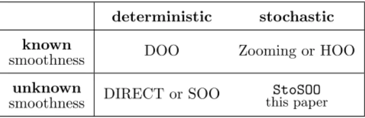
Optimistic optimization was also used in many other domains, such as planning (Hren & Munos, 2008; Bubeck et al., 2011a) or Gaussian process optimiza-tion (Srinivas et al., 2010). This paper applies opti-mistic approach to a global black-box function opti-mization. Table 1 displays representative approaches for this setting. The case when the smoothness of the functionf is known, means that the function is either (globally) Lipschitz, weakly Lipschitz or locally Lips-chitz around the optimum. There are numerous algo-rithms for this setting, the most related to our work are DOO (Munos,2011) for the deterministic case and Zooming (Kleinberg et al., 2008) or HOO (Bubeck et al.,2011a) for the stochastic one1. This setting has
been also considered in a Bayesian framework, in par-ticular the expected-improvement strategy (Osborne, 2010) which was theoretically analyzed when the as-sumption of smoothness is data-driven (Bull,2011). One of the disadvantages of these algorithms is that however strong or mild are the assumptions onf, the quantities that express them (i.e. a prior, a Lipschitz constant, or a semi-metric in DOO) need to beknown
1
Note that the loss (2) considered here is different but related to the usual cumulative regret defined in the bandit setting, see e.g. (Bubeck et al.,2009).
Table 1.Hierarchical optimistic optimization algorithms
deterministic stochastic
known
smoothness DOO Zooming or HOO
unknown
smoothness DIRECT or SOO
StoSOO
this paper
to the algorithm. On the other hand, for the case of deterministic functions there exist approaches that do not require this knowledge, such as DIRECT or SOO. However, neither DIRECT nor SOO can deal with stochastic functions. Therefore, we extend the SOO algorithm to the stochastic setting and provide a finite-time analysis of its performance.
3. Algorithm
StoSOO is a tree-search based algorithm that
itera-tively constructs finer and finer partition of the search space X. The partitions are represented as nodes of a K-ary treeT and the nodes are organized by their depthsh≥0, withh= 0 being the root node, and in-dexed by 1≤i≤Kh. We denote◦[h, i], thei-th node at depthh. Each of the nodes◦[h, i] corresponds to a cellXh,i⊆ X in the partitioning, i.e., to a subset ofX with an associated representative pointxh,i∈ Xh,i.
3.1. Assumptions
We now state our main assumption, which is also used in SOO (Munos,2011). The first part of the assump-tion is about the existence of a semi-metricℓsuch that the functionf is locally smooth with respect to it. We stress that although it quantifies the smoothness of
f, itonly requires the existence of ℓ andnot the
knowledge of it. For illustrative examples and discus-sion on this part we refer the reader to (Munos,2011). The second part is about the structure of the hierar-chical partitioning with respect toℓ. This partitioning is fixed and given to the algorithm as a parameter.
Assumption There exists a semi-metricℓ:X ×X →
IR+ (i.e. for x, y
∈ X, we have ℓ(x, y) = ℓ(y, x) and
ℓ(x, y) = 0 if and only if x=y) such that:
A1 (local smoothness off): For allx∈ X:
f(x∗)−f(x)≤ℓ(x, x∗). (3)
A2 (bounded diameters and well-shaped cells):
that for any depth h ≥ 0 and for any cell Xh,i of depth h, we have supx∈Xh,iℓ(xh,i, x) ≤ w(h).
Moreover, there exists ν > 0 such that for any depth h ≥ 0, any cell Xh,i contains a ℓ-ball of radiusνw(h) centered inxh,i.
Assumption A1 guarantees that f does not decrease too fast around one global optimum x∗. This can be thought of as a one-sided local Lipschitz assumption. Note that although we require that (3) is satisfied for allx∈ X, this assumption essentially sets constraints to the function f locally around x∗, since whenx is such thatℓ(x, x∗)>supf−inff, then the assumption is automatically satisfied. Thus when this property holds, we say thatf is locally smooth with respect to ℓ around its maximum.
AssumptionA2assures the regularity of the partition-ing, in particular that the size of the cells decreases with their depths and that their shape is not skewed in some dimensions.
3.2. Stochastic SOO
Algorithm 1 displays the pseudo-code of the StoSOO
algorithm. The algorithm operates in the traversals of the tree starting from the root down to the current depth(T), that is upper bounded byhmax, a parameter of the algorithm. During each traversal (a whole pass of the “for” cycle) StoSOO selects a set of promising
nodes, at most one per depthh. These nodes are then either evaluated orexpanded.
Evaluating a node at timetmeans sampling the func-tion in the representative pointxh,iof the cellXh,iand observing the evaluationrtaccording to (1). Expand-ing a node◦[h, i], means splitting its corresponding cell into itsK sub-cells corresponding to the children:
{◦[h+ 1, i1],◦[h+ 1, i2], . . . ,◦[h+ 1, iK]}. We denote byL the set of leaves inT, i.e. the nodes with no children. At any time, only the leaves are eli-gible for an evaluation or expansion and we never ex-pand the leaves beyond depth hmax. If the functionf were deterministic, such as in SOO (Munos,2011), we would expand (simultaneously) any leaf ◦[h, i] whose valuef(xh,i) is the largest among all leaves of the same or a lower depth. The reason for this choice is that by AssumptionA1all such nodes may containx∗. Unfor-tunately, we do not receive f(xh,i), but only a noisy estimate rt. Therefore, the main algorithmic idea of
StoSOO is to evaluate the leaves several times in
or-der to build a confident estimate of f(xh,i). For this purpose, let us define ˆµh,i(t) = Th,i1(t)Pts=1rs1{xs∈
Xh,i} the empirical average of rewards obtained at
Algorithm 1StoSOO
Stochastic Simultaneous Optimistic Optimization
Parameters: number of function evaluations n, maximum number of evaluations per node k > 0, maximum depthhmax, andδ >0.
Initialization:
T ← {◦[0,0]} {root node}
t←0{number of evaluations}
whilet≤ndo
bmax← −∞
forh= 0 to min(depth(T), hmax)do
if t≤nthen
For each leaf◦[h, j]∈ L, compute itsb-value:
bh,j(t) = ˆµh,j(t) +
p
log(nk/δ)/(2Th,j(t)) Among leaves◦[h, j]∈ Lt at depthh, select
◦[h, i]∈arg max ◦[h,j]∈L
bh,j(t)
if bh,i(t)≥bmax then
if Th,i(t)< kthen
Evaluate (sample) statext=xh,i. Collect rewardrt(s.t.E[rt|xt] =f(xt)).
t←t+ 1
else{i.e.Th,i(t)≥k, expand this node} Add theK children of◦[h, i] toT
bmax←bh,i(t) end if end if end if end for end while
Output: The representative point with the highest ˆ
µh,j(n) among the deepest expanded nodes:
x(n) = arg max xh,j
ˆ
µh,j(n) s.t. h= depth(T \ L).
state xh,i at time t, where Th,i(t) is the number of times that◦[h, i] has been sampled up to time t.
StoSOO builds an accurate estimate of f(xh,i) before
◦[h, i] is expanded. To achieve this, we define an upper confidence bound (or ab-value) for each node◦[h, i] as:
bh,i(t) def = ˆµh,i(t) + s log(nk/δ) 2Th,i(t) , (4)
where δ is the confidence parameter. In the case of Th,i(t) = 0, we let bh,i(t) = ∞. We refer to
p
log(nk/δ)/2Th,i(t) as to the width of the estimate. Now instead of selecting the promising nodes accord-ing to their valuesf(xh,i) we select them according to theirb-values bh,i.
Our algorithm is optimistic since it considers such leaves for the selection whose b-value is maximal
among leaves at depth hor lower depths, since those leaves are likely to contain the optimum x∗ at time t, given the observed samples and AssumptionA1onf. The important question is now how many times should we evaluate the node before we decide to expand it. Again, if we knew the semi-metricℓwe would be able to calculate the appropriate count for each depth h. Since we do not know it, we instead evaluate each node a fixed number ofktimes before its expansion. We ad-dress the setting ofk,hmax, andδin Sections4and5. Our analysis shows that under appropriate assump-tions onf (discussed in Section 5) we can bound the expected regret asE[Rn] =O log2(n)/√n
by setting
k=n/log3(n),hmax=
p
n/k, andδ= 1/√n.
In the algorithm, we keep track of the number of eval-uationstin order to finish when it reachesn, the maxi-mum number of evaluations, i.e., the budget. Since we are facing a stochastic setting, we cannot simply out-put the value that received the highest reward during
n evaluations, as it is the case in most of the deter-ministic approaches. Instead, we return the represen-tative pointxh,j of the node with the highest estimate ˆ
µh,j(n) among the deepest expanded nodes, i.e., such that h= depth(T \ L).
4. Analysis
In this section we analyze the performance ofStoSOO
and upper bound the loss (2) as a function of the num-ber of evaluations. We assume that the rewards are bounded2 by
|rt| ≤1 for any t. In order to derive a loss bound we define a measure of the quantity of near-optimal states, callednear-optimality dimension. This measure is closely related to similar measures (Klein-berg et al.,2008;Bubeck et al.,2008). For anyε >0, let us write the set ofε-optimal states as:
Xε def
= {x∈ X, f(x)≥f∗−ε}.
Definition 1. Theν-near-optimality dimension is the smallest d≥0 such that there existsC >0 such that for anyε >0, the maximum number of disjointℓ-balls of radius νεand center inXε is less thanCε−d.
StoSOO maintains the upper confidence bounds (b
-values) for each cell in order to decide which cell to sample or expand. We start by quantifying the proba-bility that all the average estimates ˆµh,j(t) are at any timetwithin thosebh,j(t)-values. For this purpose we
2
The analysis can be easily extended to the case when the noise is sub-Gaussian.
define the event in which this occurs and then show that this event happens with high probability.
Lemma 1. Letξbe the event under which all average estimates are within their widths:
ξdef= n∀h, i, t s.t. h≥0,1≤i < Kh,1≤t≤n,and Th,j(t)>0 : µˆh,j(t)−f(xh,j) ≤ s log(nk/δ) 2Th,j(t) o , thenP(ξ)≥1−δ.
Proof. Letmdenote the (random) number of different nodes sampled by the algorithm up to timen. Letτ1 i be the first time when the i-th new node ◦[Hi, Ji] is sampled, i.e., at timeτ1
i−1 there are onlyi−1 different nodes that have been sampled whereas at timeτ1
i, the
i-th new node ◦[Hi, Ji] is sampled for the first time. Let τs
i, for 1≤s ≤ THi,Ji(n), be the time when the
node◦[Hi, Ji] is sampled for thes-th time. Moreover, we denoteYs
i =rτs
i −f(xHi,Ji). Using this notation,
we rewriteξas: ξ= ( ∀i, u s.t. ,1≤i≤m,1≤u≤THi,Ji(n), 1 u u X s=1 Ysi ≤ r log(nk/δ) 2u ) . (5)
Now, for any i and u, the (Ys
i )1≤s≤u are i.i.d. from some distribution νHi,Ji. The node ◦[Hi, Ji] is
ran-dom and depends on the past samples (before time
τ1
i) but the (Yis)sare conditionally independent given this node and consequently:
P 1 u u X s=1 Ysi ≤ r log(nk/δ) 2u ! = =
E
◦[Hi,Ji]P 1 u u X s=1 Ysi ≤ r log(nk/δ) 2u ◦[Hi, Ji] ≥1− δ nk,using Chernoff-Hoeffding’s inequality. We finish the proof by taking a union bound over all values of 1 ≤
i≤nand 1≤u≤k.
Lemma 1 shows that when the leaf is expanded then with high probability the mean estimate ˆµh,j(t) is very close to its true value. Specifically, when the node is expanded then with probability 1−δuniformly for all
h, j,andt, we have that:
where ε = p
log(nk/δ)/2k. We use this lemma to show that the expanded nodes are with high probabil-ity close to optimal.
Definition 2. Let the expansion set at depthhbe the set of all nodes that could be potentially expanded be-fore the optimal node at depth his expanded:3
Ihε def
= {nodes◦[h, i]such that f(xh,i)+w(h)+2ε≥f∗}. Recall that even though this definition usesw(h) that depends on the unknown metric ℓ, the StoSOO
algo-rithm does not need to know it. Now, let us denoteh∗ t the deepest depth of the expanded node at timet, that contains the optimum x∗. Notice that in general the algorithm may have at timetalso expanded some (sub-optimal) nodes in the deeper depths. In the following, we show that they are not too many of these. Specifi-cally, for each depthh, we lower bound the number of evaluations after which theh∗
t needs to be at leasth.
Lemma 2. Let depthh∈ {0, hmax} be any depth and:
th def
= (k+ 1)hmax(|I0ε|+|I1ε|+· · ·+|Ihε|).
After we evaluated at least t ≥ th nodes, then in the
eventξ, the depthh∗
t of the deepest node in the optimal
branch is at leasth, i.e., h∗ t ≥h.
Proof. By induction onh. Forh= 0, the lemma holds trivially since h∗
t ≥0. For the induction step, let us assume that the lemma holds for all h ∈ {0, . . . , h′
}, where h′ < h
max and we are to show it holds forh′+ 1 as well. Assume we have already evaluated th′+1
nodes, i.e. that we are at time t ≥ th′+1. Since th is
increasing inh, we have also evaluated th′ nodes and
h∗
t ≥h′ from the induction step. That means that the optimal branch is expanded at least up to the depth
h′. Now consider any node ◦[h′+ 1, i] at depth h′ + 1, that was expanded. If it was expanded before the optimal node◦[h′+1, i∗] at depthh′+1 was expanded, then bh∗
t+1,i(t)≥bh∗t+1,i∗(t). According to Lemma 1,
the average estimates ˆµh,j(t) are at mostεaway from their true values, with ε defined in (6). Therefore in the event ξ, the true values of the expanded and the optimal node are at most 2εapart:
f(xh∗
t+1,i)≥f(xh∗t+1,i∗)−2ε. (7)
Since the node ◦[h∗
t+ 1, i∗] contains the optimumx∗, then by Assumptions A1-2, we get:
f(xh∗
t+1,i∗)+w(h+1)≥f(xh∗t+1,i∗)+ℓ(xh∗t+1,i∗, x
∗)
≥f∗.
3
The reason for such definition will become apparent in the proof of Lemma2.
Combining this with (7), we obtain that:
f(xh∗ t+1,i)≥f(xht∗+1,i∗)−2ε≥f ∗ − w(h∗ t+ 1) + 2ε .
This means that all the nodes ◦[h′ + 1, i] expanded before ◦[h′+ 1, i∗] are [w(h∗
t + 1) + 2ε]-optimal. By Definition 2, there are exactly |Iε
h′+1| such nodes. Each traversal of the tree in the StoSOO algorithm
selects one of these nodes for evaluation. Since k
evaluations are required before the expansion, after (k+ 1)|Iε
h′+1| traversals, ◦[h′ + 1, i∗] must have been
expanded. To guarantee this many traversals, we need (k+ 1)hmax|Ihε′+1|evaluations aftert′hprevious evalu-ations. This is equal toth′+1and thush∗t ≥h′+ 1. Lemma2bounds the number of needed evaluations in the terms of the expansion set sizes to assure that the optimal node was expanded. Naturally, we would like to know, how big these expansion sets can be. The following lemma upper bounds the size of expansion sets up to depth wherew(h) is of the order ofε. For this purpose, we definehε as:
hε= arg min{h∈N:w(h+ 1)< ε}. (8)
Lemma 3. Letd be aν/3-near-optimality dimension and C the related constant. Then for each h ≤ hε,
the cardinality of the expansion set at depthhis in the eventξ bounded as:
|Ihε| ≤C(w(h) + 2ε) −d
.
Proof. By contradiction. Assume that for some h ≤ hε, |Ihε| > C(w(h) + 2ε)
−d
. By definition of |Ihε|, each representative point xh,i of the node ◦[h, i] is [w(h) + 2ε]-optimal. By Assumption A2, each cell as-sociated with the node ◦[h, i] at depth h contains a ball of radiusνw(h) = ν
3 ·3w(h)≥ ν
3(w(h) + 2ε) with the representative point xh,i, because for h≤hε, we have thatε≤w(h) by (8). Since the cells are disjoint, we have a contradiction with ν/3-near-optimality di-mension being d.
We now link the depth of the tree after n iterations with the loss as defined in (2).
Theorem 1. Assume that Assumptions A1-2 hold. Let dbe the ν/3-near-optimality dimension andC be the corresponding constant. Then the loss of StoSOO
run with parameters k,hmax, andδ >0, after n
iter-ations is bounded, with probability 1−δ, as:
Rn≤2ε+w(min (h(n)−1, hε, hmax))
where ε =plog(nk/δ)/(2k) and h(n)is the smallest
h∈N, such that: C(k+ 1)hmax h X l=0 (w(l) + 2ε)−d≥n.
Proof. Let us first consider the case whenh(n)−1≤
hε. Then we can use Lemma 3to show that:
n > C(k+ 1)hmax h(n)−1 X l=0 (w(l) + 2ε)−d ≥(k+ 1)hmax h(n)−1 X l=0 |Ilε|=th(n)−1 (9) Ifh(n)−1≤hmax then by Lemma2,h∗n≥h(n)−1. If, however, h(n)−1 > hmax, then by (9) the algo-rithm has expanded all potentially optimal nodes on the level hmax and therefore h∗n ≥hmax. Nonetheless the algorithm does not go beyondhmax, so necessarily
h∗
n =hmax. Hence, in the case when h(n)−1 ≤hε,
h∗
n ≥ min{h(n)−1, hmax}. Now consider the op-posite case, i.e., when h(n)−1 ≥ hε+ 1. We can now use Lemma 3, but only up to depth hε, to get that n > thε. Similarly to the previous case, we
de-duce that h∗
n ≥ min{hε, hmax}. Altogether, h∗n ≥ min{h(n)−1, hε, hmax}. Let◦[h, j] be the deepest node that has been expanded afternevaluations. We know that h ≥ h∗
n. Let also ◦[h∗n, i∗] be the optimal node at the depth h∗n. As ◦[h, j] was expanded, the true value of its representative point and the representa-tive point of◦[h∗
n, i∗] is in the eventξat most 2εaway and therefore we conclude that:
f(xh,j)≥f(xh∗n,i∗)−2ε≥f∗−[w(h∗n) + 2ε]
≥f∗−[w(min{h(n)−1, hε, hmax}) + 2ε].
5. The important case
d
= 0
We now deduce the following corollaries for the case when the near-optimality dimensiond= 0 and the di-ameters w(h) are exponentially decreasing. We post-pone the discussion about this important case d= 0 to Section5.1.
Corollary 1. Assume that the diameters of the cells decrease exponentially fast, i.e., w(h) =cγh for some
c >0andγ <1. Assume that theν/3-near-optimality dimension is d = 0 and let C be the corresponding constant. Then the expected loss of StoSOO run with
parameters k, hmax =
p
n/k, and δ > 0, is bounded as:
E[Rn]≤(2 + 1/γ)ε+cγ√n/kmin{0.5/C,1}−2+ 2δ. (10)
Proof. When d = 0, then
w(l) + 2ε−d
= 1 and by definition of h(n), we have that n ≤ C(k + 1)hmaxPh(n)l=0
w(l) + 2ε−d
=C(k+ 1)hmax(h(n) + 1), which impliesh(n)≥n/(C(k+1)hmax)−1. Intuitively,
the deeper is the node we return, the lower regret we can incur. This suggests the choice of hmax =
p
n/k, in which case we get h(n) ≥ √n/(2C√k)−1, since
k≥1. Moreover, sincew(h) =cγh, then by definition ofhεwe have that:
w(hε) =cγhε+1/γ=w(hε+ 1)/γ < ε/γ. By Theorem1, we have that in the eventξ, the regret
ofStoSOOis at most:
Rn≤2ε+w(min{h(n)−1, hε, hmax})
≤2ε+w(hε) +w(min{h(n)−1, hmax})
≤(2 + 1/γ)ε+cγ√n/kmin{0.5/C,1}−2
We obtain the upper bound on the expected loss (10), by considering that by Lemma1,ξholds with proba-bility 1−δand|rt| ≤1.
Corollary 2. For the choice k=n/log3(n)andδ = 1/√n, we have:
E[Rn] =Olog
2 (n)
√n .
This result shows that, surprisingly, StoSOO achieves
the same rate ˜O(n−1/2), up to a logarithmic factor, as the HOO algorithm run with the best possible metric, althoughStoSOOdoes not require the knowledge of it.
Proof. Setting k =n/log3(n) and δ = 1/√n we can upper boundεin (10) which was defined in (6) as:
ε= r log(nk/δ) 2k = s log(nk√n) log3(n) 2n ≤ r 5 4 log2(n) √n .
Now for n bigger than a quantity exponential in
C/log(1/γ), the second term in (10) becomes negli-gible and the upper bound for this choice follows.
5.1. Some intuition about the case d= 0
We have seen that the near-optimality dimensiondis a property of both the function and the semi-metric
ℓ. Since StoSOO does not require the knowledge of
the semi-metricℓ(it is only used in the analysis), one can choose the best possible semi-metricℓ, possibly according to the functionf itself, in order to have the lowest possible value of d. The case d = 0 thus corresponds to the following assumption on f: there exists a semi-metricℓsuch that: 1)f is locally smooth w.r.t.ℓaround a global optimumx∗(i.e. such that (3) holds)2)the diameters of the cells (measured withℓ) decrease exponentially fast, and 3) there exists C >
0 such that for any ε > 0, the maximal number of disjoint ℓ-balls of radius νε/3 centered in Xε is less thanC (i.e. the near-optimality dimensiondis 0).
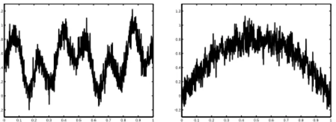
0 0.1 0.2 0.3 0.4 0.5 0.6 0.7 0.8 0.9 1 −0.2 0 0.2 0.4 0.6 0.8 1 1.2 0 0.1 0.2 0.3 0.4 0.5 0.6 0.7 0.8 0.9 1 −0.2 0 0.2 0.4 0.6 0.8 1 1.2
Figure 1.Functions with d = 0. Left: Two-sine product
functionf1(x) = 1
2(sin(13x)·sin(27x)) + 0.5.Right:
Gar-land function: f2(x) = 4x(1−x)·( 3 4+ 1 4(1− p |sin(60x)|)). 5.2. Examples
Let us consider the case of functions f defined on [0,1]D that are locally equivalent to a polynomial of degreeαaround their maximum, i.e.,f(x)−f(x∗) = Θ(kx−x∗
kα) for someα >0, where
k · kis any norm. The choice of semi-metric ℓ(x, y) =kx−ykα implies that the near-optimality dimensiond= 0. This covers already a large class of functions (such as the functions plotted in Figure 1: thetwo-sine product function for which α = 2 and the non-Lipschitz garland function for whichα= 1/2).
More generally, we consider a finite dimensional and bounded space, i.e., such that X can be packed by
CXε−D ℓ-balls with radius ε (e.g., Euclidean space [0,1]D) and such thatX has a finite doubling constant (defined as minimum value q such that every ball in
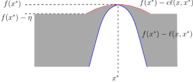
X can be packed by at most q balls in X of half the radius). Let a function in such space have upper- and lower envelope aroundx∗of the same order (Figure2), i.e., there exists constantsc ∈(0,1), andη >0, such that for allx∈ X:
min(η, cℓ(x, x∗))≤f(x∗)−f(x)≤ℓ(x, x∗). (11) We show that all such functions have a near-optimality dimensiond= 0 according to Definition1, (whereν = 1 for simplicity), which means that for all ε >0, the packing number ofXεis upper-bounded by a constant.
f(x∗) f(x∗)−cℓ(x, x∗)
f(x∗)−ℓ(x, x∗)
f(x∗)−η
x∗
Figure 2.Any function satisfying (11) lies in the gray area
and possesses a lower- and upper-envelopes that are of same order aroundx∗.
In the case when ε < η, due the upper envelope we
have that: Xε ⊂ {x : cℓ(x, x∗) ≤ ε}, which corre-sponds to an ℓ-ball centered in x∗ with radius ε/c. This ball can be packed by no more than a constant number ofC′ℓ-balls of radiusε. C′is necessarily finite because the doubling constantqis finite. For example in [0,1]D,ifℓ(x, y) =
kx−yk∞thenC′= (1/c)D. In the opposite case when ε ≥ η, the radius of dis-joint ℓ-balls that could possibly pack Xε is at least
η. Noting that Xε ⊂ X, we can upper bound the packing number of the whole spaceX, by a constant
CX(η)−D that is independent of ε. Finally, defining
C = max{C′, CX(η)−D} we have that for all ε, the maximum number of disjoint ℓ-balls of radius ε and center inXεis less than aC and therefored= 0. Even more generally, one can even define the semi-metricℓ according to the behavior of f around x∗ in order that (3) holds. For example if the space X is a normed space (with normk · k), one can define the metricℓ(x, y)def= ˜ℓ(kx−yk) for anyr≥0 as:
˜
ℓ(r) = sup x;kx∗−xk≤r
[f(x∗)−f(x)].
Thusf(x∗)
−ℓ(x, x∗) naturally forms a lower-envelope of f. Thus assuming that the first inequality of (11) (upper-envelope) holds, thend= 0 again.
However, although the case d= 0 is quite general, it does not hold in situations where there is a discrepancy between the upper- and lower-envelopes (Figure3).
Figure 3.We illustrate the case of a function with different
order in the upper and lower envelopes, when ℓ(x, y) = |x−y|α. Heref(x) = 1
−√x+(−x2
+√x)·(sin(1/x2
)+1)/2. The lower-envelope behaves like a square root whereas the upper one is quadratic. The maximum number ofℓ-balls with radiusε that can packXε (i.e., Euclidean balls with
radius ε1/α
) is at most of order ε1/2
/ε1/α
≤ ε−3/2
, since α≤1/2 in order to satisfy (3). We deduce that there is no semi-metric of the form|x−y|αfor whichd <3/2.
6. Experiments
In this section we numerically evaluate the perfor-mance ofStoSOO4. In all experiments with set the
pa-rametersk,δ, andhmaxto the values from Corollary2.
4
Moreover, we set the branching factor to K = 3. Note that when the branching factor is an odd num-ber (K ≥ 3), we can reuse the evaluations (samples) from the parent node. Indeed, if K is odd, the repre-sentative point of the parent node◦[h, i] will have the same value as the middle child◦[h+ 1,(K+ 1)/2], i.e.,
xh,i=xh+1,i(K+1)/2. In the case when the domain off
is multi-dimensional, we only need to split along one dimension at the time, when expanding the node. In order to preserve bounded diameters assumption, we can split each time along the dimension in which the cell is the largest.
For the evaluation we added a truncated (so that re-wards are bounded) zero mean Gaussian noise NT, sample of which is shown in Figure 4. In all the ex-periments we performed 10 trials and the error bars in the figures correspond to standard deviations.
0 0.1 0.2 0.3 0.4 0.5 0.6 0.7 0.8 0.9 1 −0.2 0 0.2 0.4 0.6 0.8 1 1.2 0 0.1 0.2 0.3 0.4 0.5 0.6 0.7 0.8 0.9 1 −0.2 0 0.2 0.4 0.6 0.8 1 1.2
Figure 4.Functions from Figure1noised withNT(0,0.1).
Two-sine product: In the first set of experiments we consider a two-sine product function displayed in Figure1(left) maximized forf(0.867526)≈0.975599. Figure5displays the performance ofStoSOOfor
differ-ent levels of noise. We observe that as we increase the number of evaluations, the regret ofStoSOOdecreases.
10 50 100 500 1000 0 0.05 0.1 0.15 0.2 0.25 0.3 0.35 0.4 regret (loss)
number of function evaluations
10 50 100 500 1000 −0.05 0 0.05 0.1 0.15 0.2 0.25 0.3 0.35 0.4 regret (loss)
number of function evaluations
10 50 100 500 1000 0 0.05 0.1 0.15 0.2 0.25 0.3 0.35 0.4 regret (loss)
number of function evaluations
Figure 5.StoSOO’s performance for function f1. Left:
Noised withNT(0,0.01). Middle: Noised withNT(0,0.1).
Right: Noised withNT(0,1).
10 50 100 500 1000 −0.1 0 0.1 0.2 0.3 0.4 0.5 0.6 regret (loss)
number of function evaluations
Figure 6.StoSOO
(dia-monds) vs. Stochastic DOO with ℓ1 (circles)
andℓ2 (squares) onf1.
In Figure 6, we compare
StoSOO to the
straightfor-ward stochastic version of DOO (Munos,2011), where we expand each node after log(n2/δ)/(2w(h)2) evalua-tions (i.e. when the size of the confidence interval be-comes smaller than the di-ameter w(h) of the cell).
However, (stochastic) DOO needs to know the semi-metric ℓ in order to define w(h). We evaluate the performance of this stochastic DOO using two semi-metrics that satisfy AssumptionA1: ℓ1(x, y) = 12|x−
y|(for which d= 1/2) andℓ2(x, y) = 144|x−y|2 (for which d = 0). We observe that StoSOO performs as
well as stochastic DOO for the better metric without
the knowledge of it.
Garland function: Next, we consider agarland func-tion displayed in Figure1(right). The optimization of this function is challenging becausef2is not Lipschitz for any L. However its near-optimality dimension is still d = 0 (Section 5.2). Figure 7 shows the perfor-mance of StoSOO as we vary the number of the
eval-uations. Notice a higher variance at iteration 200 in the left plot; this is because for that many iterations,
StoSOOwas able to reach the depthh= 6 but only for
a few nodes (while onlyh= 5 for less iterations) with small number of⌈200/(log3(200))⌉= 2 evaluations.
100 200 300 400 500 600 700 800 9001000 0 0.05 0.1 0.15 0.2 0.25 0.3 regret (loss)
number of function evaluations
100 200 300 400 500 600 700 800 9001000 0 0.05 0.1 0.15 0.2 0.25 0.3 regret (loss)
number of function evaluations
Figure 7.StoSOO’s performance for the garland function.
Left noised with NT(0,0.01). Right: Noised with
NT(0,0.1).
7. Conclusion
We presented the StoSOO algorithm that is able to
optimize black-box stochastic functions, without the knowledge of their smoothness. We derived a finite-time performance bound on the expected loss for the important case when there exists a semi-metric such that the near-optimality dimensiond= 0. We showed that this case corresponds to a large class of functions. In such cases, the performance is almost as good as with an algorithm that would know the best valid semi-metric. In the future we plan to derive finite-time per-formance for the cased >0.
8. Acknowledgements
This research work presented in this paper was sup-ported by European Community’s Seventh Framework Programme (FP7/2007-2013) under grant agreement no 270327 (project CompLACS).
References
Auer, Peter, Cesa-Bianchi, Nicol`o, and Fischer, Paul. Finite-time Analysis of the Multiarmed Bandit Problem. Machine Learning, 47(2-3):235–256, 2002. Bubeck, S´ebastien, Munos, R´emi, Stoltz, Gilles, and Szepesv´ari, Csaba. Online Optimization of X-armed Bandits. In Advances in Neural Information Pro-cessing Systems, pp. 201–208, 2008.
Bubeck, S´ebastien, Munos, R´emi, and Stoltz, Gilles. Pure Exploration in Multi-armed Bandits Problems.
Algorithmic Learning Theory, pp. 23–37, 2009. Bubeck, S´ebastien, Munos, R´emi, Stoltz, Gilles, and
Szepesvari, Csaba. X-armed bandits. Journal of Machine Learning Research, 12:1587–1627, 2011a. Bubeck, S´ebastien, Stoltz, Gilles, and Yuan,
Yu-Jia. Lipschitz bandits without the Lipschitz con-stant. InAlgorithmic Learning Theory, pp. 144–158. Springer, 2011b.
Bull, Adam. Convergence rates of efficient global optimization algorithms. The Journal of Machine Learning Research, 12:2879–2904, 2011.
Coquelin, Pierre-Arnaud and Munos, R´emi. Bandit Algorithms for Tree Search. InUncertainty in Arti-ficial Intelligence, pp. 67–74, 2007.
Gelly, Sylvain, Kocsis, Levente, Schoenauer, Marc, Se-bag, Mich`ele, Silver, David, Szepesv´ari, Csaba, and Teytaud, Olivier. The grand challenge of computer Go: Monte Carlo tree search and extensions. Com-mun. ACM, 55(3):106–113, March 2012.
Hansen, Eldon and Walster, William. Global Opti-mization Using Interval Analysis: Revised and Ex-panded. Pure and Applied Mathematics Series. Mar-cel Dekker, 2004.
Hren, Jean-Francois and Munos, R´emi. Optimistic Planning of Deterministic Systems. In European Workshop on Reinforcement Learning, pp. 151–164, 2008.
Jones, David, Perttunen, Cary, and Stuckman, Bruce. Lipschitzian optimization without the Lipschitz con-stant. Journal of Optimization Theory and Applica-tions, 79(1):157–181, 1993.
Kearfott, R Baker. Rigorous Global Search: Continu-ous Problems. Nonconvex Optimization and Its Ap-plications. Springer, 1996.
Kleinberg, Robert, Slivkins, Alexander, and Upfal, Eli. Multi-armed bandit problems in metric spaces. In
Proceedings of the 40th ACM symposium on Theory Of Computing, pp. 681–690, 2008.
Kocsis, Levente and Szepesv´ari, Csaba. Bandit based Monte-Carlo Planning. In Proceedings of the 15th European Conference on Machine Learning, pp. 282–293. Springer, 2006.
Munos, R´emi. Optimistic Optimization of Determinis-tic Functions without the Knowledge of its Smooth-ness. InAdvances in Neural Information Processing Systems, pp. 783–791, 2011.
Neumaier, Arnold. Interval Methods for Systems of Equations. Encyclopedia of Mathematics and its Applications. Cambridge University Press, 2008. Osborne, Michael. Bayesian Gaussian processes for
sequential prediction, optimisation and quadrature. PhD thesis, University of Oxford, 2010.
Pint´er, J´anos.Global Optimization in Action: Contin-uous and Lipschitz Optimization: Algorithms, Im-plementations and Applications. Nonconvex Opti-mization and Its Applications. Springer, 1995. Slivkins, Aleksandrs. Multi-armed bandits on implicit
metric spaces. In Advances in Neural Information Processing Systems 24, pp. 1602–1610. 2011. Srinivas, Niranjan, Krause, Andreas, Kakade, Sham,
and Seeger, Matthias. Gaussian Process Optimiza-tion in the Bandit Setting: No Regret and Exper-imental Design. Proceedings of International Con-ference on Machine Learning, pp. 1015–1022, 2010. Strongin, Roman and Sergeyev, Yaroslav.Global Opti-mization with Non-Convex Constraints: Sequential and Parallel Algorithms. Nonconvex Optimization and Its Applications. Springer, 2000.