On the Relationship between Conjugate Gradient and Optimal First-Order Methods for Convex Optimization

(1)

On the Relationship between

Conjugate Gradient and Optimal

First-Order Methods for Convex

Optimization

by

Sahar Karimi

A thesis

presented to the University of Waterloo in fulfillment of the

thesis requirement for the degree of Doctor of Philosophy

in

Combinatorics and Optimization

Waterloo, Ontario, Canada, 2013

(2)

I hereby declare that I am the sole author of this thesis. This is a true copy of the thesis, including any required final revisions, as accepted by my examiners.

(3)

Abstract

In a series of work initiated by Nemirovsky and Yudin, and later extended by Nesterov, first-order algorithms for unconstrained minimization with optimal theoretical complexity bound have been proposed. On the other hand, conjugate gradient algorithms as one of the widely used first-order techniques su↵er from the lack of a finite complexity bound. In fact their performance can possibly be quite poor. This dissertation is partially on tight-ening the gap between these two classes of algorithms, namely the traditional conjugate gradient methods and optimal first-order techniques. We derive conditions under which conjugate gradient methods attain the same complexity bound as in Nemirovsky-Yudin’s and Nesterov’s methods. Moreover, we propose a conjugate gradient-type algorithm named CGSO, for Conjugate Gradient with Subspace Optimization, achieving the optimal com-plexity bound with the payo↵ of a little extra computational cost.

We extend the theory of CGSO to convex problems with linear constraints. In par-ticular we focus on solving l1-regularized least square problem, often referred to as Basis

Pursuit Denoising (BPDN) problem in the optimization community. BPDN arises in many practical fields including sparse signal recovery, machine learning, and statistics. Solving BPDN is fairly challenging because the size of the involved signals can be quite large; therefore first order methods are of particular interest for these problems. We propose a quasi-Newton proximal method for solving BPDN. Our numerical results suggest that our technique is computationally e↵ective, and can compete favourably with the other state-of-the-art solvers.

(4)

Acknowledgements

First and foremost, I would like to express my sincere gratitude and appreciation to my supervisor, Stephen Vavasis. This thesis would have not been possible without his tremen-dous support, patience and unsurpassed knowledge. He has been a great mentor and I am extremely thankful to him.

I am also grateful to my examination committee, Henry Wolkowicz, Levent Tun¸cel, Hans De Sterck, and Michael Friedlander for their insightful comments and helpful sug-gestions.

Furthermore, I would like to acknowledge the role of the sta↵ members, the faculty members and my fellow graduate students in the department of Combinatorics and mization. I wish to specially thank the members and organizers of the Continuous Opti-mization group for the wonderful seminars and useful discussions.

Thank you to all my friends who were there for me. Particularly, I owe a heartfelt thanks to my dear friend Ali who encouraged me and lightened me up whenever I needed it the most.

Last but certainly not least, my greatest, deepest and most special thanks goes to my parents, Mehdi and Fahimeh, and my brother, Soheil, who made finishing this thesis pos-sible with their unconditional love, endless patience and continuous support. My gratitude is beyond words, but thank you for believing in me and encouraging me on this journey.

(5)

Dedication

(6)

List of Tables

2.1 Comparison of CGSO and HZ for linear log barrier function . . . 43

2.2 Comparison of CGSO and HZ for log of determinant function . . . 44

2.3 Comparison of CGSO and HZ for d-norm function . . . 44

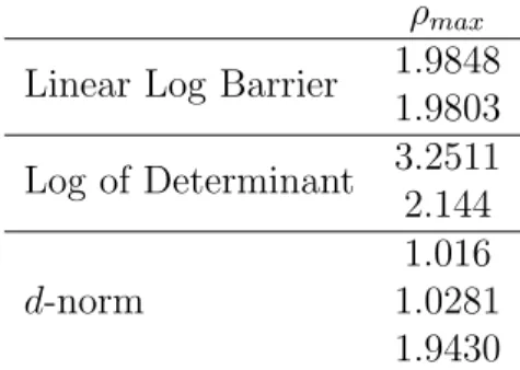
2.4 Maximum value of quotient (2.23) (¯⇢) . . . 45

2.5 Number of units of computation for convex quadratic functions. . . 47

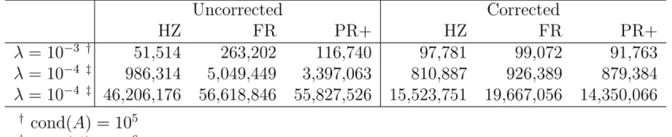
2.6 Number of units of computation for log-barrier functions. . . 48

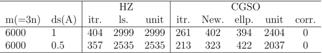
2.7 Number of units of computation for regularized BPDN functions. . . 48

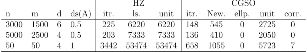
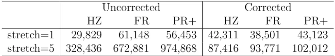
2.8 Number of units of computation for distance geometry functions.. . . 49

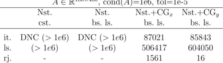
3.1 Nesterov’s method and CG for the convex quadratic function . . . 58

3.2 Nesterov’s method and CG for the smoothed BPDN problem . . . 58

5.1 Test cases with orthonormal A . . . 89

5.2 Numerical results (number ofA/At_{calls) for comparison of IMRO and NestA} ₈₉ 5.3 Information on test cases . . . 92

5.4 Numerical results (number of A/At _{calls) for BPDN solvers} _{. . . .} ₉₃

5.5 Accuracy of the solution, i.e. kxt x⇤k, in IMRO and other BPDN solvers 94 A.1 Results on CGSO for constrained problems . . . 119

(9)

List of Figures

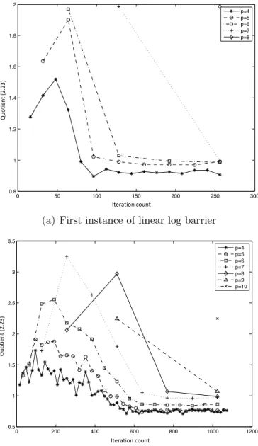
2.1 Quotient (2.23) (¯⇢) with respect to iteration count . . . 46

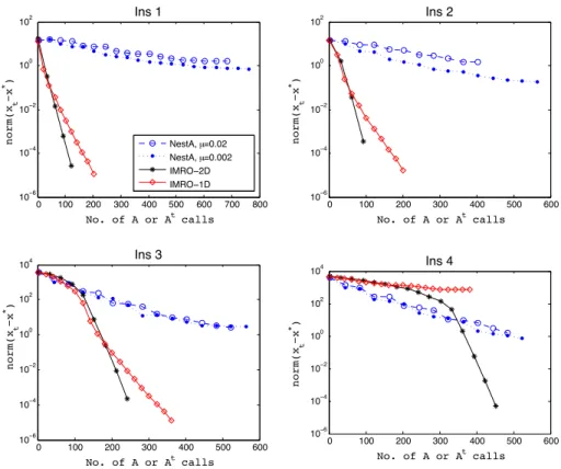
5.1 Accuracy of solution in IMRO and NestA . . . 90

5.2 Accuracy of the solution for BPDN solvers . . . 95

5.3 Recovered signal after 100 iteration for Sparco(5) . . . 96

A.1 Illustration of the sufficient reduction in objective value when _A(xj+1_{) =} A(xj₎ _{. . . 107}

(10)

Chapter 1 Introduction

The rapid progress in technology and the larger problem sizes arising in optimization call for fast, accurate and robust algorithms. For many large-scale problems, forming the Hessian is quite expensive so algorithms that rely only on function and gradient evaluations are of particular interest. These algorithms are often referred to as first-order algorithms (FOA); in other words, FOA refers to iterative algorithms that rely on information obtained by the first derivative of function in each iteration.

This dissertation is divided into two parts. The first part focuses on a class of first-order techniques for unconstrained problems called Conjugate Gradient algorithms (CG). The second part focuses on solving “Basis Pursuit Denoising Problem” (BPDN) arising in many applications including sparse recovery in compressive sensing. In the remainder of this chapter, we first present the notation and review the required background used throughout this thesis. CG methods are reviewed in Section1.2. In Section 1.3 we give a brief overview of sparse recovery and BPDN problem. An outline and the contribution of this work is discussed in Section 1.4.

1.1 Notation and Background

1.1.1 Linear Algebra

The material of this section is covered in [63, 62] in extensive detail. We reserve the lowercase alphabet for vectors, and uppercase alphabet for matrices throughout this thesis. Scalars are denoted by lowercase Greek letters. We are mainly working with real Euclidean

(11)

vector space Rn _{equipped with inner product denoted by} _h_·_,_·_i_{, and defined as} _h_{x, y}_i ₌ Pn

i=1xiyi.

A linear transformation, matrix, is defined asA :Rn_!_Rm_{. Its adjoint is denoted by} _At_, and we have _hAx, y_i = _hx, At_y_i_{. We use the standard notion of “square”, “symmetric”,} “nonsingular”, “diagonal” and “orthonormal” for matrices of sizen_⇥n. det(A),and A 1

stand for determinant and inverse of A, respectively. aij, a[i], and a[j] represent the ijth

entry, ith row, and jth column of A, respectively.

Norms:

The p-norm of a vector is defined as (Pn_i₌₁_|x_i|p₎1p. The following special cases are

partic-ularly important in our discussions:

kxk2 := v u u tXn i=1 x2 i, kxk1 := n X i=1 |xi|, kxk1:= max i |xi|.

The function _kx_k2 is often referred to as Euclidean norm, and kxk1 as l1-norm. The

following inequalities play important roles regarding vector norms:

kx+ykp  kxkp+kykp , (1.1) |hx, yi| kxk2kyk2 . (1.2)

The first inequality is the “triangle inequality”, which holds true for any norm; while the second one is “Cauchy-Schwarz inequality” and holds for Euclidean norm. In the remainder of this thesis we use_kx_k for Euclidean norm unless otherwise is stated.

Matrix induced norms are natural extensions of vector norms. Associated with any vector norm, its corresponding matrix norm is defined as:

kAkp = sup kxkp=1k Axkp = sup x6=0 kAxkp kx_kp . (1.3)

The inducedl1 and l1 norms are sometimes called maximum column sum and maximum

row sum because the induced norm formulation essentially boils down to the following equivalent forms: kAk1 = sup 1jn n X i=1 |aij| and kAk1= sup 1in n X j=1 |aij|. (1.4) The induced Euclidean or l2-norm is called the “spectral norm” and equals to

kAk2 =

p

(12)

where max stands for the maximum eigenvalue (to be defined shortly).

Note that anym_⇥n matrix can be considered as a vector of size mn, hence we can still define a component-wise matrix norm as

kAkc = m X i=1 n X j=1 |aij|c !1 c . (1.6)

Frobenius norm refers to entry-wise 2-norm for matrices. In our discussion, we use induced norms for matrices unless otherwise is stated.

Eigenvalue Decomposition and Positive Definiteness:

Scalar and nonzero vector v are called eigenvalue and eigenvector of matrix A 2 Rn⇥n if Av= v. All eigenvalues of a symmetric matrix are real numbers. A symmetric matrix can be represented by its eigenvalues asV⇤Vt_{, where}_V _{is an orthogonal matrix consisting} of eigenvectors of A, and ⇤ is a diagonal matrix with eigenvalues as the diagonal entries. A symmetric matrix A is called positive semidefinite if xt_Ax _{0 for all} _x ₂ _Rn_{; if the} inequality holds strictly for all nonzero vectors x, i.e., xt_{Ax >} _{0, then we call} _A _positive definite. Notations A _⌫ 0 and A 0 represent positive semidefinite and positive definite matrices. Also A ⌫ B and A B means A B ⌫ 0 and A B 0, respectively. All eigenvalues of a positive semidefinite matrix are nonnegative; similarly a positive definite matrix has only positive eigenvalues, so it is nonsingular. The eigenvalue decomposition enables us to define the square root of a positive semidefinite matrixA, asA12 =V⇤

1 2Vt,

where⇤12 stands for the diagonal matrix with square root of eigenvalues on the diagonal.

I and e refer to the identity matrix and all ones vector, respectively.

Definition 1.1. The scaled norm associated with a positive definite matrix H is defined as

kx_kH =

p

xt_{Hx .} _(1.7)

It is not too difficult to show that (1.7) satisfies all the axioms for a vector norm, namely • Since H 0, xt_Hx_{= 0}_,_x_{= 0,} • k↵xkH = p ↵2_xt_Hx₌_↵_k_x_k H, and • kxkH +kykH kx+ykH ,(kxkH +kykH kx+ykH)2 ,pxtHxytHy xtHy Let a = H12x, and b = H 1

2y, then the final inequality is simply Cauchy-Schwarz

(13)

Supposea and b are defined as above, then

atb =xtHy _{ k}a_kkb_k=pxt_Hxp_yt_Hy ₌_k_x_k

HkykH;

in other words the notion of Cauchy-Schwarz inequality can be extended for scaled norms as

xtHy _{ k}x_kHkykH . (1.8)

In addition, suppose min and max denote the minimum and maximum eigenvalues of a positive definiteH, then for any xwe have

minkxk  kxkH  maxkxk . (1.9)

1.1.2 Calculus and Convex Analysis

In this section we present a brief overview of convex analysis and the notions we require throughout this thesis. For detailed discussion on convex analysis, one may refer to [97,61]. The standard notations of rf(x) and r2_{f(x) are reserved for gradient and Hessian of}

function f :Rn _!_R_{. Since the algorithms discussed in this thesis are iterative methods,} we sometimes use the notation_rfk_for_r_f_(xk_{), where}_k_{is the iteration counter. Moreover} D(f) denotes the domain of a function f :Rn_!_R_{[ 1}_{, and is defined as}

D(f) =_{x:f(x)<₁_}.

The signum function is denoted by sgn, and is defined as

sgn(x)i = 8 > < > : 1 if xi <0, 0 if xi = 0, 1 if xi >0. (1.10)

Rate of Convergence:

Suppose _{xk_} _{is a sequence converging to} _x⇤_{. The sequence} {xk_} _{is said to have convergence rate of order} _p_{if there exists a constant} _m _{such that}

kxk+1 _x⇤_k

kxk _x⇤_kp m, (1.11)

for sufficiently largek. In the special cases thatp= 1 andm₂(0,1) the rate of convergence is called “linear”. When p = 2, the sequence has “quadratic” rate of convergence. A sequence converges “superlinearly” if

lim

k!1

kxk+1 _x⇤_k

(14)

Convex Sets and Convex Functions:

Set C is called convex if for any x, y 2 C and 2 (0,1), we have x+ (1 )y 2C. Let B✏(x) denote a ball of radius ✏ centred at x. The sets int(C) and rint(C) stand for the

interior and relative interior of a convex set _C which are defined as

int(C) = {x2C :9✏>0, B✏(x)✓C}, (1.13)

rint(C) = {x2C :9✏>0, B✏(x)\a↵(C)✓C}. (1.14)

A set of the form _{x:Ax_b_}is called a polyhedron. It’s not difficult to show that every polyhedron is a convex set.

Projection of a point x2Rn_{, onto a closed convex set} _C _{is defined as} Proj_C(x) = arg min

u2C ku xk. (1.15)

Let C 2 Rn _{be a set, not necessarily convex. The dual cone of} _C_{, which is always closed} and convex, is denoted by_C⇤ _{and defined as}

C⇤ =_{d:_hd, c_i 0, ₈c₂_C}. (1.16) The polar cone ofC is denoted by C and is defined as

C =_{d:_hd, c_{i }0, ₈c₂_C}. (1.17) Clearly the polar cone is equal to the negative of the dual cone, i.e.,C = C⇤_.

Similarly, the dual cone and the polar cone of a cone_K are defined as

K⇤ =_{d:_hd, c_i 0, ₈c₂_K}, (1.18) K =_{d:_hd, c_{i }0, ₈c₂_K}. (1.19) Moreover, if the cone K is closed and convex, then K=K⇤⇤_.

Theorem 1.1. [60, Theorem 3.2.5 (Moreau’s Decomposition Theorem)] Let _K be a closed convex cone. For x, y, and z in Rn_{, the following statements are equivalent:}

• z =x+y, x2K, y2K and hx, yi= 0,

(15)

The cone of feasible directions, the tangent cone, and the normal cone of a set _C at point x2C are denoted by FC(x), TC(x), andNC(x), respectively and defined as

F_C(x) = _{d:₉¯✏>0 s.t. x+✏d₂_C for ✏₂(0,¯✏)_}, (1.20) T_C(x) = ⇢ d:9{xk}✓C,{⌧k} s.t. xk!x, ⌧k!0 and x k _x ⌧k !d , (1.21) N_C(x) = _{d:_hd, x y_{i }0 for ₈y₂_C}. (1.22) A functionf is said to be convex if

f( x+ (1 )y)_ f(x) + (1 )f(y),

for each x, y ₂ _D(f) and ₂ (0,1). Any convex function is continuous over the interior of its domain. If the above inequality holds true as strict inequality for all x, y 2 D(f), x₆=y, and ₂(0,1), then the function is strictly convex.

The indicator function of a convex setC is convex and is defined as: IC(x) =

(

0 if x₂_C,

1 otherwise. (1.23)

The vector⇠ is called a subgradient of a convex function f at x2D(f) if

f(y) f(x) h⇠, y xi for all y 2D(f). (1.24) The set of all subgradients off atxis denoted by@f(x). The set@f(x) is always nonempty, closed and convex. A point x is a minimizer of f if and only if 0 lies in @f(x).

A function is said to be di↵erentiable at x if _rf(x) is the only element in @f(x). A continuously di↵erentiable function is a di↵erentiable function whose_rf(x) is a continuous function as well. Functionf belongs to the class of k continuously di↵erentiable functions if the firstk derivatives off (_rf, _r2_{f, . . . ,}_rk_f_{) exist and are continuous.}

LetCk _{stand for the class of}_k _{continuously di}_↵_{erentiable convex functions; no superscript} simply means that k = 1, i.e., the class of continuously di↵erentiable functions. The following inequality holds for a functionf ₂Cat every x, y ₂_D(f):

hrf(x) rf(y), x yi 0. (1.25) A function is called strongly convex if there exists a constantlsuch that for anyx, y 2D(f) we have

f(y) f(x) +_h⇠, y x_i+ l

2kx yk

(16)

where⇠₂@f(x). We say a function is “Lipschitz continuous with constantL” on_C _✓_D(f) if for any x, y2C and a constantL,

kf(x) f(y)_{k }L_kx y_k; (1.27) Lis called the Lipschitz constant of f. For first-order algorithms, the Lipschitz continuity of the gradient is often desired. We use the notation CL for the class of continuously di↵erentiable convex functions with Lipschitz continuous gradient. In the first part of this thesis we are primarily focused on continuously di↵erentiable strongly convex functions with Lipschitz continuous gradients, namely functions f for which we have

krf(x) _rf(y)_{k }L_kx y_k, (1.28)

f(y) f(x) +_hrf(x), y x_i+ l

2kx yk

2_. _(1.29)

We use the notation Cl,L for the aforementioned class of functions. As a result of (1.28), we have the following for a functionf ₂Cl,L:

f(y)f(x) +hrf(x), y xi+ L 2kx yk 2_, _(1.30) f(y) f(x) +hrf(x), y xi+ 1 2Lkrf(x) rf(y)k 2_, _(1.31) hrf(x) rf(y), x yi 1 Lkrf(x) rf(y)k 2_. _(1.32)

For derivation of the above inequalities one may refer to [85, Theorem 2.1.5].

Mean Value Theorem:

Let f be di↵erentiable on a convex set C. Then for any x, y₂_C we have

f(y) =f(x) +rf(x+ (y x))t(y x), for some 2(0,1). (1.33)

Taylor’s Theorem:

Let f be twice di↵erentiable on an open convex set _C. The second-order Taylor’s expansion off atx is

f(y) = f(x) +rf(x)t(y x) + 1

2(y x)

t_H(y _{x) +}_O₍_k_y _x_k3_).

Iff is di↵erentiable, one may aim for the first-order Taylor’s expansion as f(y) = f(x) +rf(x)t(y x) +O(ky xk2₎ _y ₂_C_.

(17)

Taylor’s theorem generalizes the above equations tok th di↵erentiable functions. This is however beyond the scope of our work and needs additional definitions and notations. The interested reader may refer to [80, Theorem 3.3.1].

We use the term “composite function” to refer to a function of the following form:

F(x) :=f(x) +g(x), (1.34)

wheref andg are both convex functions. Functiong is possibly non-smooth, but f ₂CL. The notion of composite function has been commonly used in the literature of first-order method for the summation of two convex functions, see for example [87, 74], and should not be confused with the composition of two functions.

Definition 1.2. [30] The projection of the steepest descent direction, i.e., rf(x), of a convex function f :_C _!R at x₂_C is denoted by _r_Cf(x) and defined as below:

rCf(x) = arg min

v {kv+rf(x)k : v 2TC(x)}. (1.35) This is often referred to as the projected gradient.

Definition 1.3. The “proximal mapping” or “proximal operator” of convex function g at

y is defined as

Proxg(y) = arg min x

⇢ 1

2kx yk

2₊_g(x) _. _(1.36)

Note that projection onto a convex setC corresponds to a proximal mapping in whichg(x) is the indicator function forC, i.e.,

Proj_C(x) = Proxg(x), (1.37) where g(x) = ( 0 x₂_C, 1 otherwise. (1.38)

The proximal point, Proxg(y), exists and is unique because 1₂kx yk2 +g(x) is strictly convex. Moreover, the proximal operator is firmly nonexpansive, i.e.,

kProxg(x) Proxg(y)k2  hProxg(x) Proxg(y), x yi 8x, y 2D(p(x)). (1.39) It is not too difficult to see why (1.39) is true. By the optimality of x, there exists a

⇠g(x)2@g(x) such that

(18)

Similarly, we have⇠g(Proxg(x)) =x Proxg(x). Using the convexity of g we get

g(Proxg(x)) g(Proxg(y)) +hy Proxg(y),Proxg(x) Proxg(y)i, (1.41) g(Proxg(y)) g(Proxg(x)) +hx Proxg(x),Proxg(y) Proxg(x)i. (1.42) Adding the above two inequalities concludes that the proximal operator is nonexpansive. Also using (1.39) and Cauchy-Schwarz inequality we derive

kProxg(x) Proxg(y)k  kx yk. (1.43)

Definition 1.4. “Shrinkage” or “Soft-thresholding” (commonly called thresholding) oper-ator refers to a proximal mapping whereg(x) is the l1-norm function, i.e.,

S (y) = arg min x ⇢ 1 2kx yk 2₊ kx_k1 . (1.44)

What makes thresholding operator interesting is the fact that it can be easily computed,

S (y)i = 8 > < > : yi yi , 0 _|yi| , yi+ yi  . (1.45)

One may easily check that (1.45) is actually equivalent to

S (y) = sgn(y) max_{|y_| ,0_}, (1.46) where denotes the entry-wise, or Hadamard product.

Using the definition of scaled norm (1.1), we can define the notion of a “scaled proximal mapping”.

Definition 1.5. The scaled proximal mapping (or operator) of a convex function g, asso-ciated with a positive definite matrixH, is defined as

ProxH_g (y) = arg min x ⇢ 1 2kx yk 2 H +g(x) . (1.47)

The properties of proximal mapping can be generalized to scaled proximal mapping. The scaled proximal point, ProxH_g (y), exists and is unique because for a positive definite matrix H the proximity function, 1₂_kx y_k2

H +g(x), is strictly convex. Besides we have ⇠g ProxHg (y) =H y ProxHg (y) ,

(19)

by optimality conditions for (1.47). We may now use the convexity of g to obtain g ProxH_g (x) g ProxH_g (y) +hH y ProxH_g (y) ,ProxH_g (x) ProxH_g (y)i, g ProxH_g (y) g ProxH_g (x) +_hH x ProxH_g (x) ,ProxH_g (y) ProxH_g (x)_i. Adding the above two inequalities gives us

kProxg(x) Proxg(y)k2H  hProxg(x) Proxg(y), H(x y)i, (1.49) which shows that the scaled proximal map is firmly nonexpansive. Using the notion of scaled Cauchy-Schwarz inequality we attain

kProxg(x) Proxg(y)kH  kx ykH. (1.50) This concludes the review on proximal operator. The interested reader can reach a more in-depth discussion on proximal operators in [7].

1.1.3 Convex Optimization

An optimization problem has the following general form: min

x2C f(x), (1.51)

wheref(x) is the objective function andC is the feasible region. Whenf is a linear function and _C is a polyhedron, the resulting problem is a linear program (LP); similarly, when f is quadratic, (1.51) is a quadratic program (QP).

An important class of problems in optimization is convex problems, in whichC is a convex set and f is a convex function. In the absence of constraints and when f ₂C, it suffices to have _rf(x⇤_{) = 0 for}_x⇤ _{to be the minimizer of} _f_{. The first order optimality condition}

for constrained convex problems requires the minimizer x⇤ to satisfy rf(x⇤) 2 N_C(x⇤). In fact, for convex problems this condition is sufficient for optimality.

It is possible to state any convex problem in the format below: min f(x)

s.t. gi(x) 0 i2{1, . . . ,I},

hj(x) = 0 j 2{1, . . . ,E},

(20)

where f(x) and gi(x) for all i = 1, . . . ,I are convex functions and hj(x) for all j = 1, . . . ,E are affine functions. The Lagrange function associated with problem (1.52) is

defined as L(x, , µ) = f(x) _I X i=1 igi(x) _E X i=1 µihi(x), (1.53) where 2 R_I _and _{0 and} _µ ₂ _R_E _{are Lagrange multipliers of problem (1.52). The}

Lagrange function is quite important in deriving optimality conditions on the minimizer of (1.52). The pointx⇤ _{is the minimizer of (1.52) if it solves}

min

x max0, µ L(x, , µ). (1.54) Problem (1.54) is called the primal problem. Its dual is

max

0, µ minx L(x, , µ). (1.55) By weak duality theorem, any feasible solution of the dual problem provides a lower bound on the primal problem. Strong duality states that the value of the primal equals the value of the dual problem at optimality. Strong duality does not necessarily hold for any convex problem. There are, however, conditions under which strong duality holds. These conditions are called constraint qualifications [90, Chapter 12]. Suppose x⇤, ? _{0, and}

µ? _{are the optimal solutions of the primal-dual problem and the constraint qualifications}

hold. Then the following set of equations is true:

rxL(x⇤, ?, µ?) = 0, (1.56a) gi(x⇤) 0 i2{1, . . . ,I}, (1.56b) hj(x⇤) = 0 j 2{1, . . . ,E}, (1.56c) ? _0, _(1.56d) ? igi(x⇤) = 0 8i2{1, . . . ,I}. (1.56e)

Conditions (1.56) called KKT conditions are sufficient optimality conditions for the class of convex problems, i.e., if KKT conditions hold, thenx⇤_,_µ?_{, and} ? _{are optimal solutions}

(21)

1.2 Conjugate Gradient Method

The method of Conjugate Gradient (CG) was introduced by Hestenes and Stiefel [59] for minimizing convex quadratic functions,

f(x) = 1 2x

t_Ax _bt_x, _(1.57)

where A 0, or A ⌫ 0 and b 2 range(A). The first order optimality conditions (i.e.,

rf(x) = Ax b = 0) imply that the solution to the above problem, x⇤, solves the linear equation Ax = b; therefore we refer to this algorithm as “linear conjugate gradient”. Hestenes and Stiefel’s original linear CG has the following form:

xj+1 =xj (r j₎t_dj (dj₎t_Adjdj, (1.58a) dj+1 = rj+1+ (rj+1) t Adj (dj₎t_Ad j dj. (1.58b)

In the above equations rj _is _r_f(xj_{) =} _Axj _b _and _d0 ₌ _r0_{, where} _x0 _{is the starting}

point. It is possible to show that the number of iterations in linear CG is bounded by the dimension of the problem, n. For more details on linear CG, one may refer to [50] or [90]. Conjugate gradient technique was soon generalized by Fletcher and Reeves [47] and Polak and Ribi`ere [92], to the general problem of unconstrained minimization, i.e.,

min

x2Rnf(x). (1.59)

However, the theoretical basis for nonlinear CG is considerably weaker than that of the linear case. In the linear case, the successive gradients are mutually orthogonal and the search directions are mutually conjugate; these facts allow several strong convergence proofs including finite termination, convergence bounded in terms of problem condition number (i.e., max(_min(_AA₎)), and superlinear convergence [50].

The general form of nonlinear CG is as follows:

xj+1 =xj+↵jdj, (1.60a)

(22)

Here,dj _{is the search direction at each iteration, and}_↵j _{is the step size, usually determined} by a line search. Di↵erent updating rules for j _{gives us di}_↵_{erent variants of nonlinear CG.} The most common formulas for computing j _are:

Fletcher-Reeves (1964): F R = kg j+1_k kgj_k , and Polak-Ribi`ere (1969): P R = ( gj+1₎t₍_gj+1 _gj₎ kgj_k .

Hager and Zhang [54] present a complete list of all updating rules in their survey on nonlinear CG. The convergence of nonlinear CG is highly dependent on the line search; for some, the exact line search is crucial. There are numerous papers devoted to the study of convergence properties of nonlinear CG, most of which discuss variants of nonlinear CG that do not rely on exact line search to be globally convergent. Al-Baali [3] shows the convergence of Fletcher-Reeves algorithm with inexact line search. Gilbert and Nocedal [48] establish the convergence of a variant of the Polak-Ribi`ere nonlinear CG algorithm with no restart and no exact line search. Dai and Yuan [39] present a nonlinear CG for which the standard Wolfe condition suffices. A recent variant of CG has been proposed by Hager and Zhang [53] that relies on a line search satisfying the Wolfe Conditions. Furthermore this algorithm has the advantage that every search direction is a descent direction, which is not necessarily the case in nonlinear CG.

From Yuan and Stoer’s perspective [116], CG is a technique in which the search direction dj+1 _{lies in the subspace of Span}_{_gj+1_{, d}j_}_{. In their proposed algorithm, they compute the} new search direction by minimizing a quadratic approximation of the objective function over the mentioned subspace. The idea of finding the next iterate of CG through a subspace optimization is the core of the variant of CG we proposed in the next chapter. It is also explored in the proposed CG techniques in [1] and [70]. A more generalized form of CG called Heavy Ball Method, was introduced by Polyak [93], in which xj+1 _is _xj₊_↵₍ _gj_{) +}

(xj _xj 1_{). He proved a geometric progression rate for this algorithm when} _↵ _and

belong to a specific range.

About two decades after nonlinear CG was originated, Nemirovsky and Yudin [82] proposed a variant of this algorithm with the worst-case complexity bound ofO(ln(1/✏)pL/l). Here

✏ is the desired relative accuracy, that is, (f(xn₎ _f_(x⇤_))/(f(x0₎ _f_(x⇤₎₎ _ _✏_{, where} _x0

is the starting point, x⇤ _{is the optimizer, and} _xn _{is the final iterate. This is the best} achievable bound for this particular class of methods and functions [82, 85]. We refer to this algorithm as NY-CG, and will cover some more details about their method in the next chapter.

(23)

Although NY-CG algorithm can be regarded as a variant of conjugate gradient, it does not reduce to linear conjugate gradient when applied to a convex quadratic function. In fact, it can be much slower. In contrast, the FR and PR variants of nonlinear CG reduce to linear CG in the case of a convex quadratic and if an exact line search is used. Many would argue that this is a defining property of nonlinear CG. In addition, NY-CG requires an expensive subspace optimization step on every iteration. A later paper by Nesterov [84] remedied this drawback by achieving the same complexity without the need for subspace optimization.

The general form of Nesterov’s algorithm is:

xk=yk ↵krf(yk), (1.61a) tk+1= 1 + p 1 + 4tk2 2 , (1.61b) yk+1 =xk+t k ₁ tk+1 x k _xk 1 _, _(1.61c) wheret0 _{= 1, and} _↵k_ 1

L is determined through a line search. If the Lipschitz constant is known, one may take the constant step size of _L1 in each iteration. Let us denote t_tkk+11 by ⌧k_{. Rewriting Nesterov’s algorithm solely in terms of sequence} _{_yk_}_{, we get}

yk+1 =yk ↵k_rf(yk) +⌧k yk ↵k_rf(yk) yk 1+↵k 1_rf(yk 1) =yk+⌧k(yk yk 1) (1 +⌧k)↵k_rf(yk) +⌧k↵k 1_rf(yk 1). Lettingdk+1

y =yk+1 yk, the above equation can equivalently be stated as

dk_y+1 =⌧kdk_y (1 +⌧k)↵krf(yk) +⌧k↵k 1rf(yk 1). (1.62) Assuming that nonlinear CG has the format mentioned in (1.60), dk+1

y in nonlinear CG would be dk_y+1 = ↵ k k ↵k 1d k y ↵krf(yk), (1.63) because yk+1 =yk+↵kdk, where dk = kdk 1 rf(yk) = k ✓ yk _yk 1 ↵k 1 ◆ rf(yk).

(24)

Comparing of (1.62) and (1.63) sheds more light on some similarities between CG and Nesterov’s algorithm. In both algorithms dk+1

y is a linear combination of the previous gradients; the di↵erence lies in the coefficients used in the linear combinations.

Despite close similarities between Nesterov’s, NY-CG, and traditional CG algorithms, the question of whether nonlinear CG can achieve the same complexity bound has remained unanswered. In Chapter 2 we derive conditions under which CG can achieve the same iteration bound of NY-CG. As a result of our study we propose an algorithm called CGSO that can achieve the same complexity bound with the cost of extra computational work per iteration.

We have already pointed out that the orthogonality of gradients does not hold for nonlinear CG, and in fact gradients may become nearly dependent causing a significant slow-down in the convergence of the algorithm. A natural measurement on the orthogonality of gradients is defined as (rf_krk)t_frk_kf2k 1 ⌫; and a normal approach to fix the dependence of gradients

is to restart CG by taking a steepest descent step. It is often believed in optimization community that the Polak-Ribi`ere variant is more robust than Fletcher-Reeves nonlinear CG. Note that when _rfk+1 _{' r}_fK_,

P R '0; thus the algorithm takes almost a steepest descent step at the next iteration. There is, however, no rigorous theory on when to restart a nonlinear CG, and how to prevent the dependence of gradients in subsequent iterations after a restart.

The theory of CGSO relies on two safeguard inequalities. Roughly speaking, one measures the amount of reduction in the objective value; while the other checks orthogonality of the gradients. Both these properties are crucial for reaching the optimal complexity bound of NY-CG. These safeguard conditions can be applied to any variant of nonlinear CG. In Section2.2 we present how these conditions can e↵ectively detect the loss of independence of gradients. Using CGSO, we also propose a technique for recovering the orthogonality of gradients. We refer to this procedure at “detection and correction” of loss of independence of gradients in CG.

1.3 Introduction to Sparse Recovery

Compressive Sensing (CS) [31, 5, 34] refers to the idea of encoding a large sparse signal through a relatively small number of linear measurements. This approach is essentially to apply a linear operator A ₂ Rm⇥n _{to a signal} _x ₂ _Rn _{and storing ˆ}_b ₌ _Ax _instead. Naturally we want ˆb 2Rm _{to be of a smaller dimension than} _{x; hence in practice}_m _⌧_n. The main question is how to decode ˆb to recover signal x, i.e., finding the solution to the

(25)

underdetermined system of linear equations

Ax= ˆb. (1.64)

Sparse recovery particularly aims at finding the sparsest solution to (1.64). The sparsest solution might be obtained by solving

min _kx_k0

s.t. Ax= ˆb, (1.65)

where _kx_k0 corresponds to the number of nonzero entries of x. Problem (1.65) is,

how-ever, NP-hard and difficult to solve, therefore the following relaxation was suggested for recovering the sparse solution:

min kxk1

s.t. Ax= ˆb. (1.66)

The theory of compressive sensing has been well-established. Candes, Tao, Romberg, and Donoho are among the pioneers of compressive sensing theory, see [32,33,42]. In fact, they have shown that under some conditions, (1.66) can recover the solution to (1.65). Note that problem (1.66) can be reformulated as an LP; however general purpose LP solvers are not a suitable choice for solving it because of the excessive run time for large instances of the problem.

In the presence of the noise in computing and storing ˆb, the in-hand measurement is often b= ˆb+ ˆ✏; hence it is customary to replace

Ax= ˆb, with

kAx b_{k }✏,

in (1.66), where ✏ is an estimated upper bound on the noise. The resulting problem is min _kx_k1

s.t. kAx bk ✏. (BP✏) (1.67)

Problem (1.66) is usually referred to as “Basis Pursuit” (BP) problem, while BP✏ refers to

its least-square constrained variant, i.e., (1.67). Other common problems in sparse recovery are

min 1₂kAx bk2₊ _k_x_k

(26)

and

min kAx bk

s.t. _kx_k1 ⌧. (LASSO) (1.69)

In the literature of compressive sensing, (1.68) is often called “Basis Pursuit Denoising Problem” (BPDN) or l1-regularized least square problem, and (1.69) goes by the name

of “LASSO” (Least Absolute Shrinkage and Selection Operator). Although in statistics, problem (1.68) is also referred to as LASSO, we stick with the customary labels used in compressive sensing.

Theoretically all the aforementioned formulations are equivalent, provided that some spe-cific relations hold true for ✏, , and ⌧. However, there is no simple manner to compute this relationship without already knowing the optimal solution. The algorithms proposed in this work are tailored for solving (1.68).

Compressive sensing has been a flourishing field of research for the last few decades. The formulations mentioned above (BP✏, BPDN, and LASSO) rises in many applications

in-cluding medical screening [79], machine learning [108], statistics [101, 118], missing data recovery [117, 99], and many other applications. One may refer to [103] for a vast list of references on the theory, applications, algorithms, and software of this field.

The key desired factors for an algorithm suited for solving any of the above formulations are speed and accuracy. Although efficient second order methods such as interior-point meth-ods [89,109,94] can achieve high accuracy, solving large-scale instances can be challenging for these algorithms. First-order methods, on the other hand, are faster and more e↵ective for solving large-scale problems rising in CS. There are numerous gradient-based first-order algorithms proposed for sparse recovery, see for example [83,46,21,57,18,114,43,110,11]. In [18, 17] an efficient root finding procedure has been employed for finding the solution of BP✏ through solving a sequence of LASSO problems. In other words a sequence of LASSO

problems for di↵erent values of is solved using a spectral projected-gradient method [22]; and as ! ?_{, the solution of the LASSO problem coincides with the solution}

of BP✏. In [114], the solution of BP problem is recovered through solving a sequence of

LASSO problems with an updated observation vectorb. GPSR [46] is a gradient projection technique for solving the bound constrained QP reformulation of BPDN.

Many other state-of-the-art algorithms in CS are inspired by iterative thresholding/shrinkage idea [37, 38, 36]. The algorithms, however, can su↵er from slow rate of convergence. Theoretically iterative thresholding algorithms have sublinear convergence in general and can achieve linear convergence only under some strict conditions [26]. The accelerated technique originally proposed by Nesterov [86] has been applied to iterative thresholding

(27)

algorithms to enhance their convergence rate, see [9] and references therein. Nesterov’s ac-celerated proximal gradient algorithm has been adopted for solving di↵erent formulations in image processing such as BP✏ in [11], LASSO problem in [52], and total variation

min-imization in [40]. Other possible approaches for solving LASSO problem are augmented Lagrangian and penalty methods as in [72] and [73], respectively. Nesterov’s algorithm is employed for solving the subproblem in both augmented Lagrangian and penalty methods. In what follows we present iterative shrinkage idea and other relevant techniques to our work in more details. Similar to the algorithms we discussed for smooth unconstrained optimization problems, algorithms discussed in this section are also iterative techniques. Recall steepest descent method as the simplest gradient based method for unconstrained problems. The general format of the generated sequence by this algorithm is:

xk+1 =x ↵_rf(xk). (1.70)

We can consider the above sequence as solutions to the following quadratic approximations of functionf, i.e., xk+1 = arg min x ⇢ f(xk) +_hx xk,_rf(xk)_i+ 1 2↵kx x k k2 . (1.71)

In the above model, one may think of

f(xk) +hx xk,rf(xk)i, (1.72) and

1

2↵kx x

k_k2_, _(1.73)

as the first order approximation to the objective function and the proximity term with weight 1

↵, respectively. If ↵ = 1

L, the model would have been the upper approximation of the objective function, and we would have the steepest descent with fixed step size. “Iterative Shrinkage Thresholding Algorithm” (ISTA) is an extension of the steepest de-scent idea to composite functions using the thresholding operator.

Consider the problem of minimizing a composite function, i.e.,

(28)

The idea of steepest descent has been extended to minimizing a composite function by simply using the same approximation model as in (1.71) for f(x). As a result we get the following iterative scheme:

xk+1 = arg min x ⇢ f(xk) +hx xk,rf(xk)i+ 1 2↵kx x k_k2₊_g(x) _. _(1.75)

Shu✏ing the linear and quadratic terms and ignoring the constant terms in (1.75), it can equivalently be written as xk+1 = arg min x ⇢ 1 2↵kx (x k _↵ rf(xk)_k2+g(x) . (1.76) Using the notion of Prox operator we conclude that

xk+1 = Prox↵g xk ↵rf(xk) . (1.77) The iterative scheme of (1.77) is “Generalized Gradient Method” or “Proximal Gradient Method”. Note that it actually coincides with steepest descent method in the absence of g(x). Finding the proximal point may not be a trivial task in general, but for solving BPDN it can be computed efficiently because the l1-norm is separable.

Iterative scheme (1.77) is often called “Forward-backward Splitting Method” [36,111]. It gets its name from the two separate stages during each iteration while minimizing (1.74); the first stage is taking a forward stepxk ↵rf(xk) involving onlyf, and the second stage is a backward step Prox↵g xk ↵rf(xk) which involves only g.

The algorithm that goes by the name of ISTA in the literature of sparse recovery is derived from the same chain of arguments for composite functions in whichg(x) = kxk1. Using

Definition1.4 an ISTA step in its general form is

xk+1 =S ↵ xk ↵rf(xk) . (1.78)

FISTA1 _[₉_{] is the accelerated variant of ISTA that was built upon the Nesterov’s idea}

[84, 86]. Each iteration of FISTA has the following format: xk+1=S 1 L ✓ yk 1 Lrf(y k₎ ◆ , (1.79) tk+1= 1 + p 1 + 4tk2 2 , (1.80) yk+1=xk+ ✓ tk ₁ tk+1 ◆ xk+1 xk . (1.81)

(29)

When no knowledge ofLis in hand, a backtracking line search is employed in (1.79). FISTA is not restricted to BPDN problem. In fact it was originally proposed for minimizing a general composite function. Replacing (1.79) with

xk+1 = Prox 1 L ✓ yk 1 Lrf(y k₎ ◆ , (1.82)

would generalize FISTA to an algorithm well-suited for minimizing composite functions. In order to incorporate more information about the function without trading o↵ the effi -ciency of the algorithms, Newton/quasi-Newton proximal methods [14, 74] has attracted researchers quite recently. Most of previous extensions on quasi-Newton methods are suited either for nonsmooth problems [75, 115], or for constrained problems with simple enough constraints [28, 98, 41]. For l1-regularization, however, proximal quasi-Newton methods

might be a more e↵ective approach.

Recall that generalized gradient method was basically derived by approximating f with a quadratic model of the form

m↵(x) = f(xk) +hx xk,rf(xk)i+ 1 2↵kx x k k2 (1.83) =f(xk) +_hx xk,_rf(xk)_i+ 1 2 x x k t ✓ 1 ↵I ◆ x xk , (1.84) and solving min m↵(x) +g(x), (1.85)

in each iteration. A natural extension of the above algorithm is to replace the diagonal matrix 1_↵I in the quadratic term ofm↵(x) with a suitable positive definite matrix. In other

words, one may define mH(x) as

mH(x) =f(xk) +hx xk,rf(xk)i+ 1

2 x x

k t_{H x} _xk _, _(1.86) whereH 0, and solve

min mH(x) +g(x), (1.87)

instead of (1.85). Ignoring the constant terms and using definition of scaled norm, we can rewrite (1.86) as mH(x) = 1 2kx x k _H 1_r_f_(xk₎ _k2 H. (1.88)

(30)

By definition of scaled proximal mapping, we can now define the proximal quasi-Newton algorithm as

xk+1 = ProxH_g xk H 1_rf(xk) . (1.89) IfH =_r2_f(xk_{) in (1.89), then we obtain the proximal Newton method.}

Alternating Direction Method (ADM), see [112,113] and references therein, is also a tech-nique that can be applied to BPDN. It is suited for minimizing the summation of (sepa-rable) convex functions, sayf(x) +g(y), over a linear set of constraints. The augmented Lagrangian technique then solves for x and y interchangeably while fixing the other vari-able. Alternating Linearization Method (ALM) [49] also applies to minimizing composite functions. In (1.75), we linearizef at every iteration to build the quadratic approximation model; in ALM a similar model based ong is also minimized at every iteration. Nesterov’s accelerated technique has also been adopted and the resulting algorithm is called FALM, for fast ALM.

A randomized first-order technique is proposed in [65] suitable for solving bilinear saddle point problem. It is, also, shown that BP✏ formulation can be transformed into an

equiva-lent bilinear saddle point formulation and solved through the proposed first-order scheme. The presented numerical results suggest that the randomization can enhance the practical performance of first-order techniques particularly for large-scale problems. This issue has attracted researchers lately and is discussed in [15] as well.

1.4 Outline of the Thesis

We mentioned in the introduction that a key question we aim to answer in this thesis is whether conjugate gradient can achieve the optimal complexity bound of Nemirovsky-Yudin’s and Nesterov’s algorithms. As a result of our study, we propose a variant of conjugate gradient algorithm named CGSO that achieves the desired complexity bound. Moreover, the analysis of CGSO suggests a new scheme for detecting and correcting the loss orthogonality of gradients in other variants of nonlinear conjugate gradient. CGSO and the detection and correction procedure for avoiding the slow-down in nonlinear conjugate gradient is presented in Chapter 2. We extend the theory of CGSO to convex problems with polyhedral constraints; and apply the resulting technique to solving the basis pur-suit denoising problem (BPDN); this result is presented in Appendix A. In Chapter 3, we review Nesterov’s optimal method for minimizing strongly convex functions. Despite its rich theory, Nesterov’s method in some cases has slower convergence than conjugate gradient methods. We present a hybrid scheme to combine conjugate gradient and Nes-terov’s method that benefits from the theory of NesNes-terov’s method as well as the practical

(31)

efficiency of conjugate gradient. In Chapter 4, we propose a novel and e↵ective proximal quasi-Newton scheme called IMRO for solving BPDN. The established theory of IMRO is not restricted to BPDN, and can be employed to the general problem of minimizing a convex function. We also present an accelerated variant of this technique that is inspired by Nesterov’s method. Chapter 5 concludes IMRO by presenting the computational ex-periment with this algorithm. Finally in Chapter6we conclude our discussion and present several venues for future work.

(32)

Chapter 2 Conjugate Gradient with Subspace

Optimization

We introduced the conjugate gradient (CG) technique in Section 1.2, and as mentioned, nonlinear CG algorithms all have the property that when applied to a quadratic objective function and coupled with an exact line search, they reduce to linear CG (LCG). For LCG we have the following results.

Theorem 2.1. [90, Theorem 5.2] Suppose _{xk_} _{is a sequence generated by the LCG for} minimizing a convex quadratic function f, then

(_rfk)tpi = 0 ₈i= 0,1, . . . , k 1,

where pi _{is the search direction at} _i_{-th iteration. Moreover} _xk _{is the minimizer of} _f _over the space of

x:x=x0+Span p0, p1, ..., pk 1 .

Theorem 2.2. [90, Theorem 5.2] At each iteration k, either xk _{is the optimal solution or} the properties below hold.

(_rfk)t_rfi = 0, for i= 0,1, . . . , k 1,

Span _rf0,_rf1, . . . ,_rfk =Span _rf0, A_rf0, . . . , Ak_rf0 ,

Span p0, p1, . . . , pk =Span rf0, Arf0, . . . , Akrf0 , (pk)tApi = 0, for i= 0,1, . . . , k 1.

(33)

Theorem 2.2 indicates that LCG finds the solution in at most n iterations. Nonlinear CG, however, has no known complexity bound when applied to nonquadratic functions. Indeed, Nemirovsky and Yudin [82] argue that their worst-case complexity for strictly convex functions is quite poor.

Nemirovsky and Yudin, on the other hand, found a di↵erent generalization of CG with worst-case complexity bound ofO(ln(1/✏)pL/l) iterations for the class of Cl,L functions. Actually, their algorithm, which we refer to as NY-CG, is not a generalization of the CG algorithm itself but rather a derivation from some equations and inequalities that underlie it: f(xk+1)_f(xk) 1 2Lkrf(x k₎ k2, (2.1a) rf(xk+1)_{? r}f(xk) +_{· · ·}+_rf(x0) , (2.1b) rf(xk+1₎_?_xk+1 _x0_, _(2.1c) hrf(xk), x⇤ xki f(x⇤) f(xk), (2.1d) ⌫f(x0) :=f(x0) f(x⇤) l 2kx ⇤ _x0_k2_. _(2.1e)

Note that in linear CG,xk+1 _{is the minimizer of} _{f(x) on the space mentioned in Theorem}

2.1, therefore the first condition is true because f(xk+1₎__f(xk 1

Lrf(x

k_{)) and} _f ₂_C

l,L.

The next two conditions follows from Theorem2.2. Fourth and fifth conditions hold true by convexity and strong convexity of function f, respectively.

As an algorithm that inherits all the mentioned properties, Nemirovsky and Yudin suggest to find iterate xk+1 _{by performing a two dimensional search on the plane passing through}

x0_{, q}k ₊_x0_{, and ¯}_xk ₌ _xk 1

Lrf

k_{, where} _qk ₌ _r_f0 ₊_{. . .}₊_r_fk_{, i.e., a general step of} NY-CG is

xk+1 = arg min

x2Ek f(x), where E

k ₌_x0_{+ Span} _qk_,_x_¯k _x0 _. _(2.2)

Clearly all of the properties listed in (2.1) hold for NY-CG method. Inequality (2.1a) holds because f(xk+1₎ _ _f(¯_xk_{); properties (2.1b) and (2.1c) are true because (}_r_fk+1₎t_qk _{= 0} and (_rfk+1₎t_x_¯K _{= 0; and the other two inequalities are properties of the function. Using} (2.1), Nemirovski and Yudin [82] showed that their method achieves the complexity bound of O(ln(1/✏)pL/l), where ✏ is the desired accuracy. Moreover, they showed that this complexity bound is optimal and can not be improved further. In other words, no first-order algorithm in which xk₂_x0_{+ Span} _r_f0_,_r_f1_{, . . . ,}_r_fk _{, can achieve a better complexity} bound for the class ofCl,L functions.

(34)

A disadvantage of NY-CG is that it has a relatively expensive computation on every iter-ation, namely, one must solve a two-dimensional convex optimization problem using the ellipsoid method[82, 105]. Although, as mentioned before, Nesterov’s algorithm [84] reme-dies this disadvantage, both NY-CG and Nesterov’s algorithm does not reduce to linear CG (and in fact, is much slower in practice). A second drawback is that both algorithms require prior knowledge of the ratio L/l. This is because they need to be restarted every O(pL/l) iterations in order to achieve the optimal complexity bound.

The purpose of conjugate gradient with subspace optimization (CGSO) is to avoid the dis-advantages mentioned above. In particular, we seek a CG-like algorithm with the following properties:

1. The algorithm should reduce to linear CG when the objective function is quadratic. 2. The algorithm should have the complexity bound ofO(ln(1/✏)pL/l) for the class of

Cl,L functions.

3. The algorithm should not require prior knowledge of any parameters describing f. 4. The cost per iteration should not be excessive.

The algorithm we propose achieves goals 1–3, and mostly achieves goal 4. It is built upon NY-CG, and like NY-CG it must solve a convex optimization subproblem on every itera-tion. The dimension of the subproblem is always at least 2 and is determined adaptively by the algorithm. The worst-case upper bound we are able to prove for the dimension of this subproblem is O(logj), where j is the number of iterations so far. However, in our testing, the dimension of the subproblem was 2 in almost all instances; in one test case it reached the value 3 for a few iterations, but it never exceeded 3. Furthermore, we find that solving the subproblem is usually fairly efficient because we usually apply Newton’s method when possible. Note that Newton’s method is not even defined for Cl,L functions in general. In a case that Newton’s method fails to be defined or fails to converge, CGSO falls back on a first-derivative method as mentioned below. However, Newton’s method in the subspace proved to be a valuable technique in practice according to our computational experiments.

Goal 3, the condition of no prior knowledge of parameters, has the obvious benefit of making the algorithm easier to apply in practice. It also has a second subtler benefit. For some convex problems, e.g., minimization of a log-barrier function, there is no prior bound onL/l over the domain of the function since the derivatives tend to infinity at the

(35)

boundaries. However, as the minimizer is approached, the bad behavior at the boundaries becomes irrelevant, and there is a new smaller ratio L/l relevant for level sets in the neighborhood of the minimizer. In this case, CGSO automatically adapts to the improved value ofL/l. Such adaptation is possible also with NY-CG, and Nesterov’s algorithm too, but, as far as we know, the adaptation must be done by the user and cannot be easily automated.

2.1 CGSO

2.1.1 The Algorithm

CGSO, in its preliminary form, is as follows: x0 _{= arbitrary;}

for j = 0,1, . . .

xj+1 ₌_xj ₊_↵j_r_f_(xj_{) +} j_dj_,

where dj ₌_xj _xj 1 _and _↵j_, j _{= arg min}

↵, f(xj +↵rf(xj) + dj)

As we shall see, some modifications are necessary to achieve the desired complexity bound. The above algorithm is certainly a generalization of nonlinear CG, since each search direc-tion is a combinadirec-tion of previous gradients. Moreover it reduces to LCG when applied to a quadratic function becausexj+1_{is the minimizer of}_f_{over the space of}_xj₊_{_r_fj_{, d}j_}_{in both} algorithms. Notice that the above algorithm is a descent method (i.e., f(xj+1₎ _ _f(xj_)), and it performs at least as well as steepest descent in each iteration. Hence it converges to a stationary point, which, for the class of convex problems, coincides with the minimizer of the function.

Let⌫f(x) denote the residual of the function, i.e., f(x) f(x⇤). By the fact thatf 2Cl,L, we get the following properties for the above algorithm

f(xj+1)f(xj) 1 2Lkrf j_k2_, _(2.3a) ⌦ rfj, x⇤ xj↵_f(x⇤) f(xj), (2.3b) ⌫f(x0) = f(x0) f⇤ l 2(x ⇤ _x0₎2_. _(2.3c)

Similar to NY-CG, property (2.3a) follows from the fact that f(xj+1₎ __f_(xj 1

Lg

j_{) and} f 2 Cl,L. Property (2.3b) is true by convexity of the function, and property (2.3c) is a

(36)

derivation from the strong convexity of f. We are now ready to present the main lemma on the complexity bound of this algorithm.

Lemma 2.1. Suppose m l8⇢qL l m and (f(xm 1₎ _f_(x0₎₎ 4 m_X1 j=0 j ! + m 1 X j=0 j⌦_r_f_(xj_{), x}j _x0↵ _<_0, _(2.4) and m_X1 j=0 j_r_f_(xj₎ __⇢ v u u tmX1 j=0 ( j₎2_kr_f(xj₎_k2_, _(2.5) are satisfied for a constant⇢, where

j ₌

s

f(xj₎ _f_(xj+1₎

krf(xj₎_k2 . (2.6)

Then the residual of the function is divided in half after m iterations; i.e., ⌫f(xm)  1

2⌫f(x 0₎_.

Before we provide the proof of the above lemma, we would like to elaborate on parameter

⇢. In the first glance at Lemma2.1, the fact thatm depends on⇢while⇢, in theory, can be as large as m might be confusing. Note that when _rfk _{is orthogonal to} _r_f0_{, . . . ,}_r_fk 1

(as in linear CG) orrf0₊_{. . .}₊_r_fk _{(as in NY-CG),} _⇢ _{is 1. Although the orthogonality} of the gradients are no longer guaranteed for CGSO, we expect that the gradients remain nearly orthogonal. Our experiment with CGSO suggests that ⇢ is normally a constant far belowm, typically two at the beginning and converging to one as we get closer to the optimizer. We will discuss more details about⇢in Section2.3.2; but for now, let us assume that ⇢is a given parameter equal to a small finite number, say less than five.

Proof. Our proof is an extension of the proof in [82, Section 7.3] in which some derivations depend on inequalities (2.1b) and (2.1c), while here we rely on inequalities (2.4) and (2.5). Suppose by contradiction that m l8⇢qL_lm, (2.4) and (2.5) are satisfied, but ⌫f(xm) > ⌫f(x0)

2 .

By definition of j_,

(37)

hence

⌫f(xj+1) =⌫f(xj) j 2

krf(xj)k2_.

Summing these equalities over j = 0,· · · , m 1, we get 0_⌫f(xm) = ⌫f(x0) m_X1 j=0 j 2_kr_f(xj₎_k2_, or equivalently, m_X1 j=0 j 2 krf(xj)_k2 _⌫f(x0). (2.7) By convexity of the function we have

⌦ rf(xj), x⇤ xj↵ f(x⇤) f(xj) = ⌫f(xj), (2.8) and so ⌦ rf(xj), x⇤ x0↵ ⌦rf(xj), xj x0↵ ⌫f(xj) ⌫f(xm)< ⌫f(x0) 2 . (2.9)

Let us consider the weighted sum of all the above inequalities for j = 0, . . . m 1 with weights j_{’s to get} *_m ₁ X j=0 j rf(xj), x⇤ x0 + _m ₁ X j=0 j⌦ rf(xj), xj x0↵< ⌫f(x 0₎ 2 m_X1 j=0 j ! , which can be rearranged to the following form

*_m ₁ X j=0 j_r_f(xj_{), x}⇤ _x0 + < ⌫f(x 0₎ 2 m_X1 j=0 j ! + m_X1 j=0 j⌦_r_f(xj_{), x}j _x 0 ↵ .

Equivalently we can rewrite the above inequality as *_m ₁ X j=0 j rf(xj), x⇤ x0 + < ⌫f(x 0₎ 4 m_X1 j=0 j ! + f(x ⇤₎ _f(x0₎ 4 m_X1 j=0 j ! + m_X1 j=0 j⌦_r_f(xj_{), x}j _x0↵ ! .

(38)

Using inequality (2.4) along with the facts thatf(x⇤₎__f_(xj_{) and} j _{0 for all}_{j, we get} *_m ₁ X j=0 j_r_f_(xj_{), x}⇤ _x0 + < ⌫f(x 0₎ 4 m_X1 j=0 j ! . (2.10)

By the Cauchy-Schwarz inequality we have

m_X1 j=0 j rf(xj) x⇤ x0 _ *_m ₁ X j=0 j rf(xj), x⇤ x0 + < ⌫f(x 0₎ 4 m_X1 j=0 j ! , hence m 1 X j=0 j_r_f(xj₎ _x⇤ _x0 _> ⌫f(x0) 4 m 1 X j=0 j ! . (2.11) By property (2.3c) we have x⇤ x0 _ r 2⌫f(x0) l . (2.12)

Furthermore, by inequalities (2.5) and (2.7) we get

m_X1 j=0 j_r_f_(xj₎ __⇢ v u u tmX1 j=0 ( j₎2_kr_f_(xj₎_k2 __⇢q_⌫ f(x0). (2.13) Replacing inequalities (2.12) and (2.13) in inequality (2.11), we get

⇢ q ⌫f(x0) r 2⌫f(x0) l > ⌫f(x0) 4 m_X1 j=0 j ! . (2.14)

Notice that by definition of and property (2.3a), j q 1

2L for all j, so m_X1 j=0 j r 1 2L m. (2.15)

Using this fact in inequality (2.14), we get

⇢q⌫f(x0) r 2⌫f(x0) l > ⌫f(x0) 4 r 1 2L m ! , (2.16)

(39)

therefore

m <8⇢

r L

l, (2.17)

which contradicts our assumption on the value ofm.

Lemma 2.1 shows that under conditions (2.4) and (2.5), the residual of the function is divided in half everym=O⇣qL

l ⌘

iterations. For the next m iterations, a further reduc-tion of 1

2 is achieved provided that (2.4) and (2.5) hold with x

m _{substituted in place of} x0_{. Hence by letting}_xm _{to be the new} _x0 _{and repeating the same algorithm, we can find}

the ✏-optimal solution in ⌃log₂ 1_✏⌥ l8⇢qL_lm iterations. Of course, m is not known to our algorithm, a point to which we return in the next section.

2.1.2 Restarting

We have already seen in the previous section that in CGSO, the residual of the function is divided in half every m iterations if (2.4) and (2.5) are satisfied. The algorithm, then, needs to be restarted with xm _{substitutes for} _x0 _{to get further reductions in the residual}

of the function. A closer look at the algorithm, however, clarifies that finding each iterate is independent of knowing x0_{. Initial point} _x0 _{is only required for checking inequalities}

(2.4) and (2.5). We use the term “restarting” to refer to the process of replacing x0 _in

inequalities (2.4) and (2.5) with xm _{for some} _{m >} _{0. Notice that this process does not} change any of the iterates, and it solely changes the interval of indices in which we check inequalities.

KnowingLandl, we can computemdirectly; hence we would be able to determine exactly when we need to restart the algorithm. In many cases, however, finding the parameters of the function is a nontrivial problem itself. In order to have an algorithm which does not rely on any prior knowledge about the function, we propose the following technique. Suppose p is an integer for which 2p _ _m _₂p+1_{. By restarting the algorithm every 2}p+1

iterations, we are guaranteed that the residual of the function is divided in half between every two consecutive restarts that contains at most 2m = d16⇢

q L

le iterates. The last statement follows from the fact that 2p+1 _ _{2m. Since the exact value of} _p _{is usually}

unknown, we repeat the above procedure for every value ofp2{'l, . . . ,'u}, where'l and 'u are lower and upper bound estimates on the value of p. Typically several values of p suffice since the size of the intervals corresponding top’s grows exponentially. Furthermore p never exceeds dlog2je, where j is the current iteration count; because inequalities (2.4)

(40)

and (2.5) are the same for all p _dlog₂j_e. We can now state the CGSO algorithm in a more complete form:

x0 _{= arbitrary,} _⇢ _given, _d0 _{= 0.} for j = 0,1, . . . xj+1 = arg min x2Ejf(x) where E j ₌_xj _{+ Span}_{_r_f_(xj_{), d}j_} Let j ₌qf(xj) f(xj+1) krf(xj₎_k2 for p='l, . . . ,dlog2je

ifj + 1 =p2p for some integer p Letrp = (p 1) 2p; check (f(xj+1₎ _f₍_xrp₎₎ 4 ⇣Pj i=rp i⌘₊Pj i=rp i_hr_f(xi_{), x}i _xrp_i_<₀ and Pj i=rp i_r_f_(xi₎ __⇢qPj i=rp( i₎2_kr_f_(xi₎_k2

If any of the above inequalities fails, take the “correction step”. (which will be defined in the subsequent section)

2.1.3 Correction Step

For convenience, let us refer to the set of iterates between two consecutive restarts as a “block” of iterates. In other words for anyp, the set of iteratesx0_{, x}1_{, . . . , x}2p ₁

is the first block of size 2p _{which we refer to as first block of} _p; _x2p

, x2p₊₁

, . . . , x2(2p_{) 1}

is the second block of p, and so on. At the end of each block we check inequalities (2.4) and (2.5). If they are satisfied and 2p l₈_⇢qL

l m

, then by Lemma 2.1 we know that the residual of the function is divided in half. On the other hand if any of these inequalities fails, then as mentioned in the previous section we need to take “correction step” for the next block of iterates. The correction step is basically computing the next block of iterates in a way that satisfaction of inequalities (2.4) and (2.5) is guaranteed for that particular block. Then the correction step is omitted in the subsequent blocks until the inequalities are violated again.

Recall that in an ordinary step, the new iterate, xj+1 _{is calculated by a two-dimensional}

search on the plane passing through xj_{, and parallel to the two-dimensional subspace} spanned by _rf(xj_), _and _dj_{. Suppose at least one of the inequalities (2.4) and (2.5) is} violated for th block of p; i.e., for the block of iterates xrp_{, . . . , x}rp+2p 1_{, where} _r