Artifact Suppressed Dictionary Learning for Low-Dose CT Image Processing

Artifact Suppressed Dictionary Learning for Low-Dose

CT Image Processing

Yang Chen, Luyao Shi, Qianjing Feng, Jiang Yang, Huazhong Shu, Limin

Luo, Jean-Louis Coatrieux, Wufan Chen

To cite this version:

Yang Chen, Luyao Shi, Qianjing Feng, Jiang Yang, Huazhong Shu, et al..

Artifact

Sup-pressed Dictionary Learning for Low-Dose CT Image Processing. IEEE Transactions on

Med-ical Imaging, Institute of ElectrMed-ical and Electronics Engineers, 2014, 33 (12), pp.2271 - 2292.

<

10.1109/TMI.2014.2336860

>

.

<

hal-01096038

>

HAL Id: hal-01096038

https://hal.archives-ouvertes.fr/hal-01096038

Submitted on 19 Dec 2014

HAL

is a multi-disciplinary open access

archive for the deposit and dissemination of

sci-entific research documents, whether they are

pub-lished or not.

The documents may come from

teaching and research institutions in France or

abroad, or from public or private research centers.

L’archive ouverte pluridisciplinaire

HAL

, est

destin´

ee au d´

epˆ

ot et `

a la diffusion de documents

scientifiques de niveau recherche, publi´

es ou non,

´

emanant des ´

etablissements d’enseignement et de

recherche fran¸

cais ou ´

etrangers, des laboratoires

publics ou priv´

es.

Abstract–_{Low-dose CT (LDCT) images are often severely} degraded by amplified mottle noise and streak artifacts. These artifacts are often hard to suppress without introducing tissue blurring effects. In this paper, we propose to process LDCT images using a novel image-domain algorithm called “artifact suppressed dictionary learning (ASDL)”. In this ASDL method, orientation and scale information on artifacts is exploited to train artifact atoms, which are then combined with tissue feature atoms to build three discriminative dictionaries. The streak artifacts are cancelled via a discriminative sparse representation (DSR) operation based on these dictionaries. Then, a general dictionary learning (DL) processing is applied to further reduce the noise and residual artifacts. Qualitative and quantitative evaluations on a large set of abdominal and mediastinum CT images are carried out and the results show that the proposed method can be efficiently applied in most current CT systems.

Index Terms_{—Low-dose CT (LDCT), dictionary learning,} noise, artifact suppression, artifact suppressed dictionary learning algorithm (ASDL)

I. INTRODUCTION

The radiation doses delivered to patients during X-ray computed tomography (CT) examinations are relatively high when compared with other radiological examinations [1]. The scanning parameters determining CT radiation dose include scanner geometry, tube current and voltage, scanning modes, length, collimation, table speed and pitch, and gantry rotation time and shielding [2]. Low dose scanning protocols (e.g. lowered mA (milliampere)/mAs (milliampere second) settings) This research was supported by National Basic Research Program of China under grant (2010CB732503), the Key Projects in the National Science & Technology Pillar Program (2013BAI01B01), National Natural Science Foundation under grants (81370040), the Project supported by Natural Science Foundations of Jiangsu Province (BK2011593), and the Qing Lan Project in Jiangsu Province. Asterisk indicates the corresponding authors.

Y. Chen, L. Shi, H. Shu and L. Luo* are with the Laboratory of Image Science and Technology, Southeast University, Nanjing 210096, China, and also with Centre de Recherche en Information Biomedicale Sino-Francais (LIA CRIBs), Rennes, France (e-mail: [email protected]; [email protected]; [email protected]; [email protected] ).They are also with the Key Laboratory of Computer Network and Information Integration (Southeast University), Ministry of Education, China.

Q. Feng and W. Chen* are with Department of Biomedical Engineering, Southern Medical University, Guangzhou 510515, China (e-mail: [email protected], [email protected]). J. Yang is with School of Optoelectronics, the Beijing Institute of Technology, Beijing, China ([email protected])

J. Coatrieux is with Centre de Recherche en Information Biomedicale Sino-Francais (LIA CRIBs), Rennes, France, and also with INSERM, U1099, Rennes, F-35000, France, and also with Université de Rennes 1, LTSI, Rennes, F-35000, France ([email protected]).

often lead to degraded reconstructed images with increased mottle noise and non-stationary streak artifacts [2–3]. Suppressing artifacts in low-dose CT (LDCT) images is rather challenging because most artifacts have position-dependent distributions and amplitudes similar to those of normal attenuating structures. Often with relatively prominent intensity features, artifacts can significantly decrease the discrimination of normal or pathological tissues. Current solutions to improve the quality of LDCT images can be roughly divided into three categories: pre-processing

approaches, iterative reconstruction algorithms and

post-processing methods.

The first one refers to those techniques that restore the projected raw data before performing standard FBP reconstructions. Adaptive filtering, multiscale penalized weighted least-squares filtering and bilateral filtering were respectively proposed in [3-5] to suppress the excessive quantum noise in projected raw data. Iterative reconstruction approaches consider the LDCT imaging as an ill-posed inverse problem, and solve the problem via the maximization or the minimization of a prior-regularized cost function using iterative type optimizations [6-18]. Many edge-preserving priors have been proposed in the past decade, for example the q-generalized Gaussian MRF (q-GGMRF) prior [8], the Huber prior [9], the total-variation (TV) based priors [10-12], the similarity based nonlocal priors in [13-14], and the normal image introduced priors for the prior image constrained compressed sensing (PICCS) algorithm in [15-18]. All these iterative methods can provide higher quality reconstructed CT images by incorporating image prior information into optimization. Effective clinical applications in LDCT have been reported for the total-variation prior (or regularization) based reconstruction, the PICCS algorithm and the adaptive statistical iterative reconstruction (ASIR) [19]. However, due to the often unavailability of well-formatted projection data from the main CT vendors, research and practical applications in this direction are sometimes limited.

Our study falls into the scope of the third category, post-processing methods, which can be directly applied on filtered back-projection (FBP) reconstructed CT images to suppress noise and artifacts. Post-processing methods have good practical applicability considering most equipped CT scanners are based on FBP algorithms. The key issue when applying post-processing on LDCT images is to obtain images with an overall perceptual quality close to the corresponding SDCT (standard-dose CT) images, and to ensure that neither important structures are lost nor new artifacts introduced.

Artifact Suppressed Dictionary Learning for

Low-dose CT Image Processing

Yang Chen,

Member, IEEE

,

Luyao Shi, Qianjing Feng, Jiang Yang, Huazhong Shu,

Senior Member, IEEE,

Limin

However, the back-projection process in FBP algorithms distributes non-stationary noise and artifacts over the whole CT image. These mottle noise and streak artifacts do not obey to specific distribution models and are difficult to remove. In the past decade, some techniques have been proposed for improving the quality of LDCT images. In [20-21], several noise reduction filters were proposed to enhance the conspicuity of lesions in abdomen LDCT images. In [22], a large-scale nonlocal means (LNLM) filter was applied to improve abdomen LDCT images with hepatic cysts by exploiting the large-scale structure similarity information. This LNLM method was further combined with a multiscale directional diffusion scheme to reduce streak artifacts in thoracic CT images [23].

A growing interest has been recently observed on sparse representations using dictionary learning (DL) [24-31]. Sparse representation and dictionary learning are closely related to each other in the framework of compress sensing theory. Compared to other restoration methods based on pixel-wise intensity update, patch-wise DL processing enables a more effective representation of patch-shaped features such as tumors or organs. Some successful applications in medical imaging have been explored for DL approaches. They concerned undersampled MRI image reconstruction [32], resolution enhancement [33], interior tomography [34], DL constrained iterative LDCT reconstruction [35], 3-D medical image denoising [36], few-views tomography [9-11, 15-17, 37], spectral CT [38] and abdomen LDCT image processing [39]. It has been widely accepted that the TV based reconstruction can also be considered a typical tomographic application of compressed sensing theory [9, 11,15, 37].

Though effective in representing patch-shaped features in LDCT image processing, the general DL based processing is ineffective in suppressing streak artifacts because the prominence of both orientation and intensity features in artifacts can lead to the same large sparse coefficients as normal tissue features in sparse coding. We will illustrate this in the following section. To overcome this, we propose an image-domain approach called artifact suppressed dictionary learning algorithm (ASDL) to improve LDCT images. The ASDL algorithm includes two steps, and performs noise and artifact reduction at different scales. In the first step, streak artifacts in LDCT images are suppressed by means of a discriminative sparse coding in high frequency bands. Three novel discriminative dictionaries are respectively designed to characterize artifact and normal tissue feature components in different orientations. Then, the second step makes use of the general DL processing to further suppress the noise and residual artifacts. Experiments on both abdominal and mediastinum data were conducted to show the improvements in image quality brought by the proposed algorithm. The structure of this paper is as follows: In section II, we describe the general DL algorithm and the proposed algorithm. Experimental settings and results are given and discussed in section III. Conclusions and plans for future work are sketched in section IV.

II. METHOD

A. The General Dictionary Learning Based Processing

Assuming the patches in the target LDCT image sparsely representable, DL based patch processing can be carried out by coding each patch as a linear combination of only a few patches in the dictionary [23-24]. This method finds the best global over-complete dictionary and represents each image patch as a linear combination of a few dictionary vectors (atoms). The coefficients of the linear combination can be estimated through the sparse coding process described in [25]. Based on the terminology used in [26-27], the DL based patch processing aims to solve the following problem:

2 2 2 0 2 , , min ij ij ij ij x Dαλ x

−

y +

∑

_ij µ α +

∑

_ij R x−Dα (1)

Where, x and y denote respectively the m-pixel in the

processed image and in the original LDCT image. The subscript ij indexes each image pixel index (i, j). Rij

represents the operator that extracts the patch xij of size

n× n (centered at (i, j)) from image x. The patch-based

dictionary D is a n K× matrix, which is composed of K

n-vector atoms (columns). Each n-vector column corresponds to one n× n patch. αdenotes the coefficient set

{ }

αij _ij for all the sparse representations of patches, and each patch can be approximated by a linear combination Dαij⋅||

α

ij||₀denotes the

0

l norm that counts the nonzero entries of vector αij. Based on [28], solving Eq. (1) includes the following two steps including Eq. (2) and Eq. (3):

2 2 0 0 , min s.t. , α

α

−

α

≤

ε α

， ≤ ∀ ij D ij R x D ij ij L i j (2) 2 2 2 2 min_x λ − +

∑

ij −

α

ij ij x y R x D ₍₃₎

Eq. (2) aims to train the coefficients α and dictionary D

from a set of image patches and can be efficiently solved by the K-means Singular Value Decomposition (K-SVD) with the

replacement of x by the known observed image y [28].

Starting from an initial dictionary (e.g. the DCT dictionary, which is obtained by sampling the cosine wave functions in

different frequencies), this K-SVD operation estimates α

and D by alternatively applying two steps: (i) the Sparse Coding Step using the orthogonal matching pursuit (OMP) algorithm and (ii) the Dictionary Update Step based on SVD

decomposition. The columns of the target dictionaryDare

constrained to be of unit norm to avoid scaling ambiguity in calculation [28]. The ε _{in Eq. (2) denotes the tolerance}

parameter used in calculating α _{by the OMP method and is}

modulated with respect to the level of noise/artifact level. L

limits the number of atoms in the representation of each patch. Parameter L in Eq. (2) ensures that the atom number does not exceed a certain number in each representation, even if the tolerance constraint is not met. Then, with fixed dictionaryD

and α, we can obtain the output image x by solving Eq. (3) through zeroing the first order derivative of Eq. (3) with respect to image x:

1 T T ij ij ij ij ij ij x λI R R λy R Dα −     =_ + _{ } + _ 

∑

 

∑

 (4)

The dictionary can also be pre-trained from a typical SDCT image before LDCT processing. It has been validated in [39] that a global dictionary can lead to almost the same result as the dictionary trained from the LDCT image itself. Besides, using a pre-trained dictionary will save considerable computation cost in the overall processing. With a

pre-calculated dictionary D_p (obtained via solving Eq.(2)

using some other SDCT images) chosen as the global dictionary, the whole DL processing can be transformed into the following two steps:

0 2 2 0 (S1), min s.t. , , α

∑

αij ij − pαij ≤ε αij ≤ ∀ ij R x D L i j (5) 2 2 2 2 (S2), minλ − +

∑

_ij − _pα_ij x ij x y R x D (6)

Here, the sparse coefficient αcan be solved via Eq. (5) using the OMP algorithm. The image x in Eq.(6) can be calculated via above Eq. (4).

As pointed out above, streak artifacts are found hard to be suppressed via the DL method. Fig.1(b) illustrates one typical LDCT image section with strong artifacts, and Fig.1(c) is the result of the DL processing using the global dictionary in Fig.1 (a). Parameters in the DL method were adjusted to provide the best visual result in terms of noise/artifact suppression and structure preservation. In the DL processed LDCT image in Fig.1(c) we can observe obvious residual artifacts. Applying more aggressive parameters to remove all the artifacts would lead to blurred details.

Fig.1 (a), the global dictionary trained from a typical SDCT image; (b), one typical LDCT image section with strong streak artifacts; (c), the corresponding DL processed LDCT image section.

B. Artifact Suppressed Dictionary Learning Algorithm

The assumption for the general DL algorithm relies on the fact that normal tissue structures always lead to significantly larger sparse coefficients than such undesirable features as noise or artifacts. Unfortunately, using the feature dictionary atoms showed in Fig.1(a), streak artifacts in LDCT images can also be linked to large sparse coefficients, and are thus hard to be differentiated from normal anatomical structures in the general DL processing.

Fig.2 illustrates the high frequency bands of one typical LDCT abdomen image and the corresponding SDCT image from the best matched slice in another SDCT scan. We can see in Fig.2 that most streak artifacts show directional and oscillating patterns in high frequency domain. Better artifact suppression can be expected if it is performed for different orientations in high frequency domain. Also, the directional features of artifact can be used to build specific atoms to get a discriminative processing in sparse representation. From these intuitive observations, we propose in this paper a ASDL

(b)

(c)

(a)

Fig.2 (a1) is one typical LDCT image; (a2)-(a4) are the horizontal, vertical and diagonal high frequency bands of the LDCT image, repectively; (b1) is the corresponding SDCT image, and (b2)-(b4) are the corresponding high frequency bands of the SDCT image.

(a4) (a2) (a3) (b4) (b2) (b3) (a1) (b1)

approach based on a novel concept of discriminative dictionary. The idea behind discriminative dictionary is to obtain an integrated dictionary containing both artifact atoms and normal tissue feature atoms, which can be independently trained from pre-selected artifact and feature samples. Effective artifact suppression can then be achieved by simply setting those artifact sparse coefficients (related to artifact atoms) to zero in the image solving step in Eq.(6). This operation is named Discriminative Sparse Representation (DSR).

The stationary wavelet transform (SWT) is used in this work to preserve translation-invariance in decomposing the LDCT images into two scales (high frequency scale and low frequency scale). The high frequency scale includes the three bands for horizontal, vertical and diagonal orientations. It is found the three orientation bands in high frequency scale can well represent most high frequency artifact components. The Haar wavelet is here used in SWT for it is fast and found to suffer less from the so-called “ringing” or pseudo-Gibbs artifacts than other wavelet forms with wider filter bases [22]. We first construct artifact samples (as given in Fig.3(b), (d) and (f)) by manually extracting artifact patches from ten typical abdomen LDCT images in the three high frequency bands. Artifact patches were first carefully selected under the guidance of an experienced doctor (X.D.Y. with 15 years of experience) from background regions in the original LDCT image to avoid the inclusion of image details. Considering that translation-invariance (point to point correspondence) is well preserved in SWT, we can easily obtain the background regions in wavelet domain by choosing exactly the same

background regions specified in the original image. From

Fig.4 Illustration of the discriminative dictionaries for the high frequency bands with different orientations. The first, second and third row show the concatenated dictionaries , and for horizontal, vertical and diagonal bands, respectively.

Horizontal

Vertical

Diagonal

Fig.3 Demonstration of the training samples in this study. (a) is one typical SDCT image. (b), (d) and (f) are the extracted artifact samples in the three high frequency bands collected from ten typical LDCT images; (c), (e) and (g) are the corresponding high frequency feature samples extracted from the SDCT image in (a).

(b) (c)

(d) (e)

(f) (g)

these artifact patches, we trained three artifact dictionaries a chd D , a cvd D and a cdd

D for the three bands. Also, we trained

three tissue feature dictionaries Dcvdf , f cvd

D and Dcddf

using the high frequency bands (as given in Fig.3(c), (e) and (g)) obtained from one typical SDCT images (as given in Fig.2(a)). The K-SVD algorithm in [28] is used to train the

dictionaries via solving Eq.(2) and Eq.(3). Three

discriminative dictionaries ( d chd D , d cvd D and d cdd D ) can be

built by concatenating the artifact and feature dictionaries:

[ | ], d a f chd chd chd D = D D d [ a | f ] cvd cvd cvd D = D D and

D

_cddd

=

[

D

_cdda

|

D

_cddf

]

. In this study, as illustrated in Fig.3, the cardinals of feature and artifact dictionaries are both set to 450 (M=450) to guarantee redundancy in sparse representation.

We can see in Fig.4 that all the discriminative dictionaries include both the artifact atoms (left part, from artifact dictionary) and the feature atoms (right part, from feature dictionary). The orientation and textural information for image features and artifacts can be distinctly observed in Fig.3. Then, given the discriminative dictionaries displayed in Fig.4, the overall ASDL algorithm is implemented based on the flowchart in Fig.5 and the outline in Fig.6. The original LDCT image is first decomposed via SWT into three high frequency bandsfchd,fcvd,fcdd and one low frequency band fca. In the

DSR operation with the discriminative dictionaries d

chd D , d cvd D and d cdd

D , tissue features are prominently related to

sparse coefficients from feature atoms whereas artifact features to sparse coefficients from artifact atoms. Artifact suppression is performed by setting the first M coefficients linked to artifact atoms in discriminative dictionaries to zero. Then the artifact suppressed bands fchd,fcvd,fcdd are built via the same way given in Eq.(4). In this process, tissue features can be well preserved because the sparse coefficients related to feature atoms are kept. Following the artifact suppression step for high frequency bands, the Inverse Stationary Wavelet Transform (ISWT) with Haar wavelet is carried out to retrieve the artifact-suppressed image from the artifact suppressed high frequency bands and the original low frequency band. The final restored image can be obtained by applying the general DL processing on the artifact suppressed image via above Eq.(2)-(4) to deal withnoise and residual artifacts.

It is found in Fig.4 that the trained artifact dictionaries are composed mostly by the atoms characterizing artifact features. Nevertheless, some image feature information (e.g. fine edges)

can be introduced into artifact dictionaries, which leads to suppressed image features. Subtraction between LDCT and SDCT images of a static anthropopathic phantom might give more exclusive artifact samples for training. But we currently do not have such anthropopathic phantoms, and a simple modularized phantom cannot provide CT images with the artifact textures in clinical patient images.

Training Discriminative Dictionaries: train three

artifact dictionaries a chd D , a cvd D and a cdd D from

extracted artifact samples and three feature dictionaries f chd D , f cvd D and f cdd

D from extracted feature samples

using the K-SVD algorithm. Two kinds of dictionaries are then merged into three discriminative dictionaries

[ | ], d a f chd chd chd D = D D d [ a | f ], cvd cvd cvd D = D D d [ a | f ] cdd cdd cdd D = D D . Suppressing Artifacts: Loop: repeat T times

 Image Decomposition: perform stationary wavelet

decomposition on the original LDCT image f_{, in}

order to get the high frequency bands fchd,fcvd,fcdd and low frequency band fca.

 Sparse Coding: with d

chd D , d cvd D and d cdd

D , calculate the corresponding sparse

coefficients αchd, αcvdand αcdd for fchd, fcvd and cdd

f using OMP method.

 Artifact Suppression: set the first M rows of αchd, cvd

α and αcdd to zero and obtain

p α = [ p chd α , p cvd α , p cdd

α ]. Then compute the artifact suppressed band

images fchd , fcvd , fcdd as 1 T T p ij ij ij ij ij ij I R R y R D λ λ α − + +         

∑

 

∑

.

 Inverse Wavelet Transformation: build artifact

suppressed image f from fchd,fcvd,fcdd and fca.

Suppressing noise and residual artifacts: apply the

general DL algorithm to suppress the residual noise and

artifacts in f and obtain the final processed LDCT

image fˆ.

Fig.6 Outline of the ASDL algorithm.

Though different artifact samples lead to different trained dictionary atoms, the artifacts in LDCT images for different Fig.5 The flowchart of the proposed ASDL method. � denotes the input degraded LDCT image. �_�� denotes the decomposed low frequency band. ��ℎ�,����,���� and �̅�ℎ�,�̅���,�̅��� respectively denote the original and artifact suppressed high frequency bands in horizontal, vertical and diagonal

orientations. �̅ denotes the artifact suppressed image from the ISWT operation of all the bands (�_��, �̅_�ℎ�,�̅_���,�̅_���). �̂ is the finally restored LDCT image after applying the DL processing on �̅ to suppress residual noise and artifacts.

SWT Input LDCT image � ���� ���� ��ℎ� ��� ��� �̅�ℎ� �̅��� �̅��� ISWT �̅ Restored LDCT image�̂ DL DSR DSR DSR

human parts share common directional patterns. So the trained dictionaries from abdomen CT images are expected to be able to be used in processing CT images of other human body parts. We validate this with study on mediastinum CT data.

III. EXPERIMENT RESULTS

A. Experiment Settings

Abdomen and mediastinum CT images were acquired in DICOM from a multi-detector row CT unit (Siemens SOMATOM Sensation 16 CT scanner). 32 and 24 patients were involved in abdomen and mediastinum data collection, respectively. We classified the whole 56 patients into abdomen scanning group and mediastinum scanning group. The abdomen scanning group includes 14 women and 18 men with an average age of 65.4 years (age range: 52-82 years). The mediastinum scanning group includes 11 women and 13 men with an average age of 62.8 years (age range: 50-77 years). Approval of this study was granted by our institutional review board. Data collection and processing were conducted according to the authorized protocol. All the patients have given their written consent to the participation. A non-conflict of interest for this work was also declared. The CT images were exported as DICOM files and then processed offline under a PC workstation (Intel Core™ i7-3770 CPU and 8192 Mb RAM, GPU (NVIDIA GTX465)).

Radiation dose was controlled by modulating the tube

current time products [milliampere second (mAs)] [2]. LDCT and SDCT images were from the scans with a reduced tube current 40mAs and the routine tube current 160mAs, respectively. Some scan protocol parameters are as follows: kVp, 120; slice thickness, 6mm; reconstruction method, FBP algorithm with convolution kernel “B70f” or “B30f”. In FBP algorithm, the parameter of convolution kernel is used to control contrast preservation and artifact/noise suppression. In FBP reconstruction, compared with kernel “B30f”, kernel “B70f” can provide CT images with more detail information but more severe artifacts and noise. For brevity, we denote the

FBP reconstruction with B70f and B30f to FBPB70f and

FBPB30f, respectively. Other scanning parameters were set by

default. In this study, to provide initial images with rich structure information, the LDCT images reconstructed from FBPB70f algorithm were chosen for processing. In order to

have reference images for evaluation, we reconstructed SDCT images with kernel “B30f” because “B30f” is the routine kernel setting for Siemens CT imaging in abdomen and mediastinum windows. LDCT images from FBP with kernel “B30f” were also provided for comparison. The recorded accumulated doses represent each scan with 40 slices in the

form of CTDIvol (volume CT dose index) for each CT

examination. The averaged recorded CTDIvol are 12.48mGy

(milligray) and 3.12mGy for each SDCT and LDCT scan, respectively. The AS-LNLM method and the global dictionary based general DL processing have shown good artifact or noise suppression in [23] and [39], and were conducted for comparison purpose.

Parameters for all the methods are listed in TABLE I. The involved parameters for the AS-LNLM and ASDL methods were specified under the control of one radiological doctor (X.D.Y. with 15 years of experience) to provide the best visual results. We practically found that the same parameter setting can be well used to process the LDCT images with the same scan protocol. The AS-LNLM method involved 7 parameters to set, namely: the total decomposition scale S of SWT, K,

Iter and inc for the nonlinear diffusion, the decaying

parameter h and the values of n and N for the LNLM

processing. For the general DL method, the sparsity limit L0

is set to 5 atoms; the dictionary size is set to 256 atoms (K0

=256) for 8×8 patch (n0=64). The global dictionary for

general DL processing is pre-trained from the SDCT in Fig.2(b1) based on [39] using parameters as follows: 20 iterations are used in dictionary training (Iter=20); sparsity limit LT is set to 5 atoms; the dictionary size is set to 256

atoms (KT=256) for 8×8patch (nT=64); tolerance parameter T

ε

in Eq.(5) is set to

_{5.8 10}

×

4 _{. The proposed ASDL}

method include three parts -- DT (dictionary training), DSR processing in wavelet domain, and the following general DL operation. Though pre-trained dictionaries are routinely used in this study, we list the involved parameters for dictionary training in the DT row in TABLE I to provide the complete information for the proposed algorithm. The trained discriminative dictionaries in Fig.4 is used in all the processing; 20 iterations are used to train each dictionary (Iter=20); the sparsity limit L1 is set to 8 atoms; sizes M for

artifact and feature dictionaries are both set equally to 450; n1

is set to 256 (for 16×16patch); the tolerance parameter ε1 in

discriminative sparse coding is set to 300 to give an accurate approximation with the discriminative dictionaries; Parameter λ in Eq.(6) is set to 25 and the artifact suppression operation is performed twice (T=2) to reduce residuel noise and artifacts. For the second step in ASDL method, the general DL processing with the same dictionary in Fig.1(a) is used, and the parameters are set as follows: sparsity limit L2 to 5 atoms;

TABLEI

PARAMETER SETTINGS FOR DIFFERENT METHODS IN EXPERIMENT

Methods Abdomen data Mediastinum data

AS-LNLM 2, 200, 10 S= K= Iter= 20, 0.05,8 8 , h= inc= × n 81 81 × N 1, 100, 10 S= K= Iter= 5, 0.05,8 8 , h= inc= × n 81 81 × N General DL 0 0 20, 5, 256 Iter= L = K = 5 0 64, 0 4.14 10 n = ε = × 10 λ = 0 0 20, 5, 256 Iter= L = K = 5 0 64, 0 3.05 10 n = ε = × 10 λ = A S D L DT DSR: Iter=20,LT=8,MT =450,nT =256,εT =300 DL: Iter=20,LT =5,KT=256,nT =64,εT =5.8 10× 4 D S R 1 8, 450, 1 256, L = M= n = 1 300, 25,T 2 ε = λ= = 1 8, 450, 1 256, L = M = n = 1 300, 25,T 2 ε = λ= = DL 2 5, 2 256, 2 64 L = K = n = 4 1 7.6 10 , 50 ε = × λ= 2 5, 2 256, 2 64 L = K = n = 4 1 4.1 10 , 50 ε = × λ=

the dictionary size to 256 atoms (K2=256) for 8×8patch (n2

=64); tolerance parameter

ε

2 in Eq.(5) to

4

7.6 10× and

4

4.1 10× for the abdomen and mediastinum data, respectively. Parameter λ is set to 50.

The abdomen window (center, 50HU; width, 350HU) and mediastinum window (center, 0HU; width, 350HU) are respectively used in the illustrations for abdomen and

mediastinum data. The AS-LNLM processing was

implemented based on [22] using GPU parallelization technique in a CUDA framework. We practically found that the GPU technique is ineffective in accelerating the OMP calculation due to the asynchronous stopping of the sparse coding for each patch. So we resort to accelerating the loop calculations in both the general DL method and the proposed Fig.7 Illustraion of artifact suppression in high frequency bands (wavelet domain). (a1)-(c1): for the LDCT image, the horizontal high frequency band, the vertical high frequency band and the diagonal high frequency band. (a21)-(c2): for the corresponding SDCT image, the horizontal high frequency band, the vertical high frequency band, the diagonal high frequency band. (a3)-(c3): the artifact suppressed high frequency bands of the LDCT image from the DSR operation. (a4)-(c4): the high frequency bands computed with only the coefficients for artifact atoms.

(a1) (b1) (c1) (a2) (b2) (c3) (b3) (a3) (c2) (a4) (b4) (c4)

ASDL method by using MATLAB Parallel Computing

ToolboxTM where multicore CPUs can be fully employed [40].

B. Illustration of Artifact Suppression in Wavelet Domain

Fig.7 illustrates artifact suppression in wavelet domain for the proposed ASDL approach. Fig.7(a1)-(a3) and (b1)-(b3) display the decomposed high frequency bands of a typical abdomen LDCT image and the corresponding SDCT image. Fig.7(c1)-(c3) show the results after applying the DSR operation to suppress the high frequency artifact components of the LDCT image. With the high frequency bands of the SDCT image as reference, we can see that the high frequency artifact components of LDCT image can be effectively reduced through the proposed DSR operation with discriminative dictionaries. Also in Fig.7(d1)-(d3), we illustrate the images calculated with only the coefficients related to artifact atoms in the discriminative dictionary. We can see that the images in Fig.7(d1)-(d3) mainly contain the high frequency artifact features, which confirms the correlation between artifact atoms and the artifact features in LDCT images.

C. Visual Assessment

Fig.8 and Fig.9 show the processing results on the same abdomen LDCT image of an 84 years old man with hepatic metastases (pointed by red arrows), and Fig.10 shows the result for a mediastinum LDCT image of a 70 years old man with lung cancer (pointed by red arrows). Fig.8 gives the results after each steps in the ASDL implementation. Fig.8(a)-(d) are the original LDCT image, the result after the first DSR operation, the result after the second DSR operation, and the final processed image after DL processing. We can observe a progressive improvement of image quality at each step, and that the DSR operation can give effective artifact suppression. Fig.9(a) and Fig.10(a) are the original FBPB70f

reconstructed LDCT images. Fig.9(b) and Fig.10(b) are the

corresponding reference original SDCT images from FBPB30f

reconstruction. The results of the general DL method and the proposed ASDL methods are given in (c) and (f) in Fig.9 and Fig.10, respectively. Additionally, in Fig.9(d) and Fig.10(d), we provide the LDCT images processed twice using the general DL method with the same parameters as the General DL method in TABLE I. Also, in Fig.9(e) and Fig.10(e), we provide the LDCT images processed twice using the general DL method, the first using the same parameters for the general DL method in TABLE I and the second using the parameters of the DL step in the ASDL method in TABLE I. In Fig.9-10, (e)-(h) illustrate the zoomed regions of interest (ROI) specified by the red squares in (a). By comparing (a) and (b) in Fig.9-10, we can see that, under LDCT scanning condition, mottle noise and streak artifacts severely degrade the reconstructed images and lower tissue discrimination. As shown in Fig.9-10 (c), the general DL method is not only ineffective in suppressing streak artifacts but also leads to obvious structure ambiguity. We can also see in (d) and (e) in Fig.9 and Fig.10 that an additional DL prcessing can also lead to successful artifact suppression, but tend to significantly smooth normal image structures. It can be observed in (d) in

Fig.9 and Fig.10 that our ASDL approach performs much better in both noise and artifact suppression, and can produce images with visual illustration similar to the reference SDCT images in Fig.9(b) and Fig.10(b).

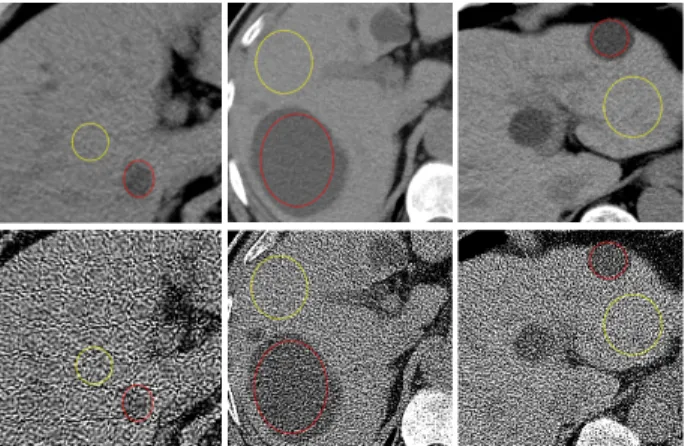
Fig.11 provides the processing results for abdomen CT images of four adult patients and Fig.12 the processing results for mediastinum CT images of another four adult patients. Zoomed image sections are also given below. The first, second, third, fourth and fifth columns in the Fig.11-12 (except the

second row) correspond to the FBPB70f reconstructed LDCT

images (a1, a2, a3, a4), the reference FBPB30f reconstructed

SDCT images (b1, b2, b3, b4), the FBPB30f reconstructed

LDCT images (c1, c2, c3, c4), the AS-LNLM processed LDCT images (d1, d2, d3, d4) and the ASDL processed LDCT images (e1, e2, e3, e4). To be specific, the first row (al, b1, c1, d1, e1) in Fig.11 illustrates the CT images with hepatic cysts (pointed by red arrows in a1) and the second row provides the difference images between the resulting LDCT images and the original FBPB70f reconstructed LDCT images; the third and the

fourth rows (a2, b2, c2, d2, e2, a3, b3, c3, d3, e3) show two cases with hepatic metastases (pointed by red arrows in a2 and a3); the fifth row (a4, b4, c4, d4, e4) illustrates the images from one healthy patient with the red arrows pointing to the biliary ducts. As to Fig.12, the first row (al, b1, c1, d1, e1) illustrates the images with esophageal cancer (pointed by red arrow in a1) and the second row the difference images

between the processed images and the original FBPB70f

reconstructed LDCT images; the third and the fourth row (a2, b2, c2, d2, e2, a3, b3, c3, d3, e3) depict two cases with mediastinal lymph nodes (pointed by red arrows in a2 and a3); the fifth row (a4, b4, c4, d4, e4) illustrates the images with lung cancer (pointed by red arrow in a4).

In Fig.11-12, with the SDCT images (b1, b2, b3, b4) as reference, we observe that the mottle noise and streak artifacts severely degrade the LDCT images of FBPB70f (a1, a2, a3, a4),

and the FBPB30f algorithm leads to smoother textures (c1, c2,

c3, c4) but with obvious noise/artifact residuals in the LDCT images. We can also see in (d1, d2, d3, d4) that the AS-LNLM method reduces noise and artifacts but at the same time tends to introduce some striped artifacts (see the yellow arrows in d1 and d2 in Fig.11-12). Significant improvements of image quality (e1, e2, e3, e4) are achieved by using the proposed ASDL method without introducing such artifacts, and the processed results present textures visually closer to the reference SDCT images. Especially, the ASDL approach improves the conspicuity of both anatomical tissues and pathological changes (e.g. the location specified by the red arrows in Fig.11-12) better than the AS-LNLM processing and the FBPB30f reconstruction. In the second rows in Fig.11-12,

comparing the difference images with respect to the original LDCT images, we can observe the strongest artifacts/noise components (see the yellow circles in the second row in Fig.11) in the difference images between the original LDCT images and the ASDL processed results. This observation confirms that the ASDL method can lead to more effective artifact/noise suppression. Even though, we can still observe a few residual artifact traces in the ASDL processed images (pointed by the yellow arrows in the most right colums of Fig.11-12). This is

due to the fact that some high contrast artifacts also have prominent components in low frequency bands. Fig.8. Step by step result in the ASDL implementation of one 84 years old man with hepatic metastases (pointed by red arrows) in abdomen window. (a), the original FBPB70f reconstructed LDCT image; (b), result after the first DSR operation; (c), result after the second DSR

operation; (d), the final result after the DL operation ; (e)-(h) show the zoomed ROI in (a)-(d).

(a) LDCT image (b) Result after the frist DSR operation

(c) Result after the second DSR operation (d) Final processed image

Fig.9 Processing result of one 84 years old man with hepatic metastases (pointed by red arrows) in abdomen window. (a), the original FBPB70f reconstructed LDCT image; (b), the reference FBPB30f reconstructed SDCT image; (c), the

general DL processed LDCT image; (d), the LDCT image processed twice using the general DL method , both using the same parameters for the general DL method in TABLE I; (e), the LDCT image processed twice using the general DL method, where the first processing uses the parameters for the general DL method in TABLE I and the second uses the parameters of the DL step for the ASDL method in TABLE I; (f), the ASDL processed LDCT image; (g)-(l) show the zoomed ROI in (a)-(f).

(a) LDCT image (b) SDCT image

(c) General DL processed LDCT image

(f) ASDL processed LDCT image (e) General DL twice processed LDCT image II

(d) General DL twice processed LDCT image I

(g) (l) (j) (k) (i) (h)

Fig.10 Processing result of one 70 years old man with lung cancer (pointed by arrows in (e)) in mediastinal window. (a), the original FBPB70f reconstructed LDCT image; (b) the reference FBPB30f reconstructed SDCT image; (c), the general DL

processed LDCT image; (d), the LDCT image processed twice using the general DL method, both using the same parameters for the general DL method in TABLE I; (e), the LDCT image processed twice using the general DL method, where the first processing uses the parameters for the general DL method in TABLE I and the second uses the parameters of the DL step for the ASDL method in TABLE I; (f), the ASDL processed LDCT image; (g)-(l) show the zoomed ROI in (a)-(f).

(a) LDCT image (b) SDCT image

(f) ASDL processed LDCT image (c) General DL processed LDCT image

(i) (l) (h) (g) (k) (j)

(e) General DL twice processed LDCT image II

Fig.11 Processing result of four adult patients in abdomen window. The first, second, third, fourth and fifth columns correspond to the original FBPB70f

reconstructed LDCT images (a1, a2, a3, a4), the reference FBPB30f reconstructed SDCT images (b1, b2, b3, b4), the FBPB30f reconstructed LDCT images

(c1, c2, c3, c4), the AS-LNLM processed LDCT images (d1, d2, d3, d4) and the ASDL processed LDCT images (e1, e2, e3, e4). The second row illustrates the difference images between the resulting LDCT images and the original LDCT image in the first row.

(a1) (b1) (d1) (a1)-(c1) (a3) (b3) (a4) (b4) (e4) (c1) (e1) (a1)-(d1) (a1)-(e1) (a2) (b2) (c2) (d2) (e2) (d3) (c3) (e3) (c4) (d4)

Fig.12 Processing result of four adult patients in mediastinal window. The first, second, third, fourth and fifth columns correspond to the FBPB70f

reconstructed LDCT images (a1, a2, a3, a4), the reference FBPB30f reconstructed SDCT images (b1, b2, b3, b4), the FBPB30f reconstructed LDCT

images (c1, c2, c3, c4) ,the AS-LNLM processed LDCT images (d1, d2, d3, d4) and the ASDL processed LDCT images (e1, e2, e3, e4). The second row illustrates the difference images between the resulting LDCT images and the original LDCT images in the first row.

(a3) (d3) (a4) (b4) (c4) (d4) (e4) (a1) (b1) (c1) (d1) (e1) (b2) (c2) (a1)-(d1) (a2) (d2) (e2) (c3) (b3) (a1)-(e1) (a1)-(c1) (e3)

D. Comparison with Iterative Reconstruction Algorithm

We compared the proposed ASDL method with typical iterative reconstruction algorithms. Both simulated phantom and clinical patient data are considered in this part.

As to the experiment on simulated phantom data, a

monoenergetic CT model with fanbeam geometry

configuration was simulated. The detector cell spacing is set to 1 mm. The detectors arrays are located on an arc concentric to the X-ray source with a distance of 949 mm, and the distance of the rotation center to the arc detector band is 408 mm. The detector cell spacing is 1 mm. 360 projection views are evenly spanned on a circular orbit of 2π and the number of bins for each projection view is 729. Thus, the simulated sinogram size is 729×_{360. Noise-free projection data along the rays through}

the phantom are computed based on the known intensities and the intersection areas of the rays with the inside geometric objects. Based on [41-42], the calibrated and log-transformed projection data of LDCT protocols follow approximately a Gaussian distribution, the relation between the mean and variance being: 2 _exp s ρ η   = × _{ }   d d g (7) where

g

_d and

s

_d denote respectively the mean and variance of the projection data at detector d. We obtained the simulated LDCT projection data (sinogram) by adding Gaussian noise to the noise-free sinogram with a variance given by Eq.(7). The

ρ and η were set to 2

1.5 10× and _{4.5 10}× 4 _{in this study.}

We simulated the corresponding LDCT sinogram by setting

the total photon count number to 8

5 10× . Fig.13(a) and (c) illustrate the simulated sinogram data for the phantom images in Fig.14(a) and Fig.15(a), which are respectively a modified Shepp-Logan phantom image and an elliptical phantom image. Fig.13(b) and (d) show the simulated noisy (LDCT) sinogram data corresponding to the true singroam data in Fig.13(a) and (c). Especially, the elliptical phantom image includes two hot regions (white) and one cold region (black), and the hot circle region in the right part shows gradual intensity variation into the background. Such gradual intensity variation can simulate tissue infiltrations along organ or lesion boundaries in realistic

clinical abdomen CT. Both the two 512×512 phantom

images (pixel size: 1mm× 1mm) have intensity values

ranging from 0 (HU) to 300 (HU). We performed FBP with

the Hanning filter (FBPhanning) to produce an image with

visually similar contrast levels as clinical abdomen images

reconstructed by FBPB30f. We also performed FBP with Ramp

filter (FBPramp) and the iterative reconstruction of L1-norm TV minimization in [9] and [15]. The half-interval based minimization technique in [15] was used to solve the TV

regularized optimization in reconstruction. In TV

reconstruction, the FBPramp reconstructed LDCT image is

used as the initial image, and the total iteration number is set to 500 to ensure a stable iteration. The hyperparameter of TV terms is chosen from 0.02 to 0.08 to depict the relationship between artifact suppression and hyperparameter values. Around 20 minutes are required to perform one TV reconstruction with 500 iterations. ASDL processing with the same parameters as in above abdomen studies was applied on

the FBPramp reconstructed LDCT images, which contains high

contrast intensity information like above FBPB70f

reconstructed LDCT clinical images.

Experimental results on on phantom data are displayed in the window [0HU, 300HU] in Fig.14 and Fig.15. In Fig.14 and Fig.15, (b) and (c) illustrate the FBPramp and FBPhanning reconstructed LDCT images where obvious noise and artifacts can be observed. We can see that both the Ramp and Hanning filters cannot successfully suppress artifacts in FBP reconstructions. Fig.14(d) and Fig.15(d) show the results

obtained after applying the ASDL algorithm on the FBPramp

reconstructed LDCT images in Fig.14(b) and Fig.15(b). The proposed ASDL approach appears effective in suppressing noise/artifacts and the processed LDCT images (Fig.14(d) and Fig.15(d)) present a good visual quality with respect to the phantom image in Fig.14(a) and Fig.15(a). Images (e)-(f) in Fig.14 and Fig.15 illustrate the images from TV reconstruction with hyperparameter ranging from 0.02 to 0.08. We can see that, through iterative optimization with TV regularization, images with effective contrast preservation and noise/artifact suppression can be reconstructed. We can see larger hyperparameters of TV term lead to more effective suppression of noise and artifacts in homogenous regions. But

Fig.13 the simulated singroam data for the phantom images. (a) and (b) are the true and simulated LDCT sinograms for the phantom image in Fig.14(a). (c) and (d) are the true and simulated LDCT sinograms for the phantom image in Fig.15(a).

we also find TV regularization tends to introduce new staircase artifacts in the region with gradual intensity variation (see the arrows in the zoomed images in Fig.15). And such staircase artifacts cannot be removed by increasing the hyperparameter values.

Below the reconstructed images in Fig.14, we list the signal-to-noise ratio (SNR) and the structural similarity index comparisons (SSIM) calculated with respect to the reference phantom images. The SSIM metric was proposed in [43] as a robust image quality metric that can give a good overall Fig.14 Comparison with TV based iterative algorithm for phantom image 1. (a), SDCT reference image; (b), LDCT image reconstructed by FBP with ramp filter (FBPramp), with PSNR 8.73 and SSIM 0.14; (c), LDCT image reconstructed by FBP with hanning filter (FBPhanning), with PSNR 14.82 and

SSIM 0.37; (d), ASDL processed LDCT image of (b), with PSNR 18.35 and SSIM 0.93; (e), LDCT image reconstructed by TV reconstruction, with PSNR 18.81 and SSIM 0.84; (f), LDCT image reconstructed by TV reconstruction, with PSNR 20.48 and SSIM 0.94; (g), LDCT image reconstructed by TV reconstruction, with PSNR 20.90 and SSIM 0.97; (h), LDCT image reconstructed by TV reconstruction, with PSNR 20.83 and SSIM 0.97.

(a) (b) (c) (d)

(e) (f) (g) (h)

Fig.15 Comparison with TV based iterative algorithm for phantom image 2. (a), SDCT reference image; (b), LDCT image reconstructed by FBP with ramp filter (FBPramp), with PSNR 8.97 and SSIM 0.06; (c), LDCT image reconstructed by FBP with hanning filter (FBPhanning), with PSNR 16.50 and

SSIM 0.31; (d), ASDL processed LDCT image of (b), with PSNR 23.05 and SSIM 0.93; (e), LDCT image reconstructed by TV reconstruction, with PSNR 22.40 and SSIM 0.90; (f), LDCT image reconstructed by TV reconstruction, with PSNR 24.55 and SSIM 0.98; (g), LDCT image reconstructed by TV reconstruction, with PSNR 24.68 and SSIM 0.97; (h), LDCT image reconstructed by TV reconstruction, with PSNR 24.96 and SSIM 0.98.

(a) (b) (c) (d)

consideration of feature preservation. The calculations of PSNR and SSIM are given in Eq. (8) and (9):

( )

(

)

2

(

)

2 10 10 PSNR , log j- - j j j j m m P x =



_

P P P x



_



∑

∑



(8)

(

)

2 2 2 2 2 1 2 (2 2 SSIM , )( ) ( )( ) Px P x Px cs P x P x cs cs s s s = + + + + + (9)

where, _P and

_x

denote the reference phantom image and the LDCT images to evaluate. m denotes the total pixel number.

_P

and

_x

denote the mean intensities of images P and

x

. sP and sx are the standard deviation

of images P and

x

. sPx is the covariance of images P

and

x

, 2

1

=

(

Ks Ls

1

)

cs

and 2

2

=

(

Ks Ls

2

)

cs

with

Ls

the

range of the HU values (300 for the range 0HU to 300HU in this phantom study), and Ks1and Ks2 are set to 0.01 and

0.03 based on [43]. We can see that, among all the LDCT images, the TV reconstructed LDCT images obtain the highest values in both SNR and SSIM metrics.

Fig.16 draws the intensity profiles along the red dotted lines indicated in Fig.14(a) and Fig.15(a) for the reconstructed images. Fig.16 shows that the ASDL method and TV reconstruction lead to LDCT images with a much better match to the phantom images than the FBP results. We can also observe that the TV reconstruction method can give the best restoration of the homogenous regions (see the red arrows in Fig.16 (c1) and (c2)). Here too, the proposed ASDL method gives a good restoration of the region with gradual intensity variation (see the green arrows in Fig.16 (d2)).

From above we can find TV based iterative reconstruction

performs well in both homogeneous region restoration and sharp edge preservation. The highest SNR and SSIM metrics are attributed to the fact that wide-distributed homogenous regions in phantoms can be well restored via the TV regularization in iterations. But the TV based iterative reconstruction also tends to introduce new staircase artifacts in the region with gradual intensity variation, and the reason is that the pairwise neighboring intensity differences in TV regularization often cannot provide enough information for discriminating noise/artifacts from fine image structures. From Fig.14-15, we can see that new staircase artifacts tends to be introduced by TV regularization into the regions with subtle intensity variations, and such staircase artifacts are free in the ASDL processed results. In clinical CT images, such regions often contain important disgnostic information. Another drawback of TV reconstruction is the high computation cost involved (20 minutes per 2-D slice in this case).

Clinical images were collected with a GE Discovery CT750 HD CT scanner under low dose tube current setting (40mAs), and the reconstructions performed by means of the FBP algorithm with sharp filtering and the iterative ASIR 100% algorithm, which are two built-in algorithm options in GE Discovery CT750 HD CT [19]. Visual comparison with ASIR reconstruction for the clinical data is reported in Fig.17 in abdomen window. Fig.17(a1) and (a2) illustrate the original FBP reconstructed LDCT images. Fig.17(b1) and (b2) show the corresponding ASIR reconstructed LDCT images. The ASDL processed LDCT images are given in Fig.17(c1) and (c2). We can see the iterative ASIR algorithm is able to reduce noise but appears not effective in suppressing high-contrast artifacts. Here too, the present method performs better for both noise/artifact suppression and patchy tissue conspicuity (see the red arrow in Fig.17(c2)) than the ASIR algorithm.

(a1) (a2)

Fig.17 Comparison with iterative reconstruction algorithm for clinical CT images. (a1) and (a2), FBP reconstructed LDCT images; (b1) and (b2), ASIR reconstructed LDCT images; (c1) and (c2), ASDL processed result for the LDCT images in (a1) and (a2).

(a1) (b1) (c1)

(b2)

(a2) (c2)

Fig.16 Illustration of the intensity profiles along the two red dotted lines indicated in Fig.14(a) and Fig.15(a). (a1) and (a2), comparison between FBPramp reconstructed LDCT image and the reference phantom image; (b1) and (b2), comparison between FBPhanning reconstructed LDCT image

and the reference phantom image; (c1) and (c2), comparison between the LDCT image reconstructed by TV algorithm and the reference phantom image; (d1) and (d2), comparison between the ASDL processed LDCT image and and the reference phantom image. (a1), (b1), (c1) and (d1) correspond to the vertical dotted line in Fig.14(a), and (a2), (b2), (c2) and (d2) correspond to the horizontal dotted line in Fig.15(a)

(c1) (c2)

E. Quantitative Assessment

First, it should be noted that the clinical LDCT and the corresponding SDCT images have no exact spatial correspondence to each other because of the inevitable displacements caused by patient breath and movements in scans. This makes it impossible to fully quantify image quality using some Euclidean distance metrics (e.g. the mean squared error (MSE)). So we chose to compare the standard deviation (STD) of specified regions of interest (ROI) and background regions in both the original and processed LDCT images with respect to those of the reference SDCT images. Three groups of image data were selected from the above patient datasets. Under the guidance of one radiological doctor (X.D.Y. with 15 years of experience), the ROIs were selected to include the pathological tissues, and the background regions were delineated out from the regions outside ROIs. Fig.18 illustrates the ROI (surrounded by red circles) and background regions (surrounded by yellow circles) for the original SDCT and LDCT images from three abdomen datasets. We calculated the STD of the ROI and background regions for both the original and processed CT images via Eq. (10):

(

)

2 Ω 1 STD 1 p p ij ij x x_Ω ∈Ω = − Ω −

∑

(10) p ij

x

and

x

_Ωp denote each point intensity and the averaged intensity of all the pixels within Ω, respectively. TABLE II lists the calculated STD of the tumor and background regions specified in Fig.18. Tumor-k and background-k (with k equal to 1, 2 and 3) correspond respectively to the regions defined in the CT images of the first, second and third columns in Fig.18. We can clearly note in TABLE II that the ASDL processed LDCT images obtain closer STD values to those of the SDCT images than the original FBP reconstructed LDCT images

(FBPB70f and FBPB30f) and also the AS-LNLM processed

LDCT FBPB70f images.

In addition, Fig17(c), (d), (e) and (f) plot the histogram maps (in black) of the specified ROI (the red box in the LDCT

image in Fig.19(a)) for the FBPB70f reconstructed LDCT

images, the FBPB30f reconstructed LDCT images, the

AS-LNLM processed LDCT images (FBPB70f) and the ASDL

processed LDCT images (FBPB70f), respectively. The

reference ROI histogram map within the red box for the corresponding SDCT image is illustrated in Fig.19(b). In Fig.19(c), we can observe a large histogram discrepancy between the ROI in the original LDCT and the reference

SDCT images. We can also see that, when compared with the

AS-LNLM processing and the FBPB30f algorithm, the ASDL

processing leads to the ROI with the closer histogram match with the corresponding ROI in the SDCT image.

(a) (b)

(c) (d)

(e) (f)

Fig.19 The histogram maps (black) of the tumor region for the FBPB70f

reconstructed LDCT image, the FBPB30f reconstructed LDCT image, the

AS-LNLM processed LDCT image and the ASDL processed LDCT images. The histogram map of the corresponding ROI in the original SDCT image in (b) is overlaid (in red color) on other histogram maps.

Fig.18 The three columns from left to right illustrate the selected ROI and background regions from three abdomen CT image datasets. In each column, the upper and lower images denote the SDCT image and the corresponding LDCT image, respectively.

TABLE II

STDS OF ROI AND BACKGROUND REGIONS FOR THE ORIGINAL LDCT

IMAGES, THE ORIGINAL SDCT IMAGES AND THE PROCESSED LDCTIMAGES

LDCT _(FBP B70) Reference SDCT (FBPB30) LDCT (FBPB30) AS-LNLM processed LDCT (FBPB70) ASDL processed LDCT (FBPB70) ROI-1 86.09 15.41 19.26 17.12 16.65 Background-1 85.30 8.33 17.99 13.26 10.98 ROI -2 89.10 8.73 17.75 11.34 9.65 Background-2 80.86 8.33 17.21 10.19 8.86 ROI -3 88.54 8.80 18.11 11.07 8.62 Background-3 109.46 11.43 23.31 15.14 11.66

F. Qualitative Assessment

The qualitative assessment includes 150 original images (25

abdomen LDCT images (FBPB70f), 25 abdomen LDCT images

(FBPB30f), 25 mediastinal LDCT images (FBPB70f), 25

mediastinal LDCT images (FBPB30f), 25 abdomen SDCT

images (FBPB30f) and 25 mediastinal SDCT images (FBPB30f)),

and 100 processed images (25 AS-LNLM processed abdomen LDCT images, 25 AS-LNLM processed mediastinal LDCT images, 25 AS-LNLM processed abdomen LDCT images and

25 ASDL processed mediastinal LDCT images). Only FBPB70f

reconstructed LDCT images were considered for processing with AS-LNLM and ASDL methods. The quality of all the images were assessed using 5 subjective features: noise suppression, artifact suppression, contrast preservation, tissue discrimination and overall image quality using a 5-point

subjective criterion (1=unacceptable, 2=substandard,

3=acceptable, 4=above average, 5=excellent). Here, we define artifacts as any pattern influencing the diagnosis passively. Three radiological readers (X.D.Y. with 15 years of experience, X.H.Y. with 8 years of experience, Y.M.D. with 5 years of experience.) independently evaluated the randomized LDCT images, SDCT images, the AS-LNLM processed LDCT images and the ASDL processed LDCT images on a digital DICOM archiving/assessing workstation (ViewDEX 2.0 [44]). In this way, the 5 subjective features were assessed for all the 250 images (150 original CT images, and 100 processed CT images), and this results in a total of 3750

parameter ratings (250×₅×_{3=3750). For each subset of}

images, the 5 image scores were reported as means±_SDs

(averaged scores of the 3 radiologists±_{standard deviations).}

The subjective quality parameters of the original LDCT images and the processed LDCT images were compared with those of the corresponding SDCT images and the differences between each two groups were evaluated by the Student t test (Excel; Microsoft) with P<0.05 considered as a statistically significant difference.

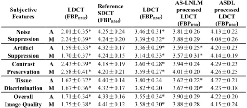
As illustrated in TABLE III, the original LDCT images obtain much lower quality scores than the reference SDCT images and also the processed LDCT images (P<0.05). The FBPB30f reconstruction and the AS-LNLM processing lead to

higher subjective scores than the FBPB70f reconstruction. The

best performance, for all scores, is obtained for the ASDL processed LDCT images. Statistically significant differences (P<0.05) with respect to the reference SDCT images are noticed in all the subjective scores for the original FBPB70f

reconstructed LDCT images, in artifact suppression and tissue discrimination for the AS-LNLM processed LDCT images, and in all the subjective scores except the tissue discrimination for the FBPB30f reconstructed LDCT images (P<0.05). The

differences between the proposed ASDL processed LDCT images and the corresponding SDCT images for the 5 subjective scores are found not statistically significant (P>0.05). TABLE III shows that the ASDL processed LDCT images even achieve higher scores in contrast preservation than the reference SDCT images. The is due to the fact that the B30f kernel in FBP might blur some image details in the SDCT images.

G. Computation costs

TABLE IV lists the computation costs (in seconds) for the different methods. We should note that both the general DL method and the proposed ASDL method include dictionary training step and OMP step. In our experiment, it takes 9.66 seconds to train a dictionary for the general DL method. Since six dictionaries (three artifact dictionaries and three tissue feature dictionaries) must be trained and the size of each 11 dictionary is larger than that of the general DL method (450 compared with 256), the training step in DSR operation of ASDL processing is rather computational intensive and takes

about 121.92 seconds. Fortunately, the dictionaries, once

trained, can be used to process all the LDCT cases as demonstrated in the above experiments. TABLE IV shows the average computation costs required in the operations following the dictionary training only. We can see that, with the trained dictionary available, the general DL method and the proposed ASDL method requires about 0.83 and 17.60 seconds to process one 512 512× slice, respectively. We can see the ASDL method is much more time comsuming than the general DL method because of the more involved DL relevant operations for different scales.

TABLE III

IMAGE QUALITY SCORES ( mean±SDs)WHERE A STANDS FOR ABDOMEN DATA AND M STANDS FOR MEDIASTINAL DATA

Subjective Features LDCT (FBPB70f) Reference SDCT (FBPB30f) LDCT (FBPB30f) AS-LNLM processed LDCT (FBPB70f) ASDL processed LDCT (FBPB70f) Noise Suppression A 2.01±0.35* 4.25±0.24 3.46±0.31* 3.81±0.26 4.13±0.22 M 2.24±_{0.39* 4.24}±_{0.20 3.39}±_{0.32* 3.88}±_{0.29 4.08}±_0.26 Artifact A 1.59±0.33* 4.32±0.17 3.36±0.29* 3.59±0.25* 4.20±0.23 Suppression M 1.70±0.37* 4.24±0.15 3.14±0.33* 3.57±0.31* 4.14±0.19 Contrast A 2.43±_{0.39* 4.18}±_{0.19 3.60}±_{0.28* 3.94}±_{0.24 4.29}±_0.23 Preservation M 2.58±0.41* 4.20±0.21 3.59±0.27* 4.01±0.20 4.26±0.25 Tissue A 1.62±0.32* 4.40±0.14 3.80±0.24 3.62±0.22* 4.27±0.21 Discrimination M 1.67±_{0.36* 4.32}±_{0.17 3.82}±_{0.20 3.67}±_{0.20* 4.23}±_0.18 Overall A 1.71±_{0.34* 4.33}±_{0.16 3.55}±_{0.34* 3.90}±_{0.29 4.22}±_0.20 Image Quality M 1.75±0.38* 4.41±0.12 3.58±0.30* 3.88±0.28 4.15±0.24

* Significantly different from the mean scores for the reference SDCT images (P<0.05).

TABLE IV

THE AVERAGE COMPUTATION COST (IN SECONDS) FOR THE AS-LNLM

METHOD IN [23], THE DL METHOD IN [39] AND THE PROPOSED ASDL METHOD

AS-LNLM General DL ASDL