Clustering
Clustering
Definition
A form of unsupervised learning, where we identify
groups in feature space for an unlabeled sample set
•
Define
class regions in feature space using unlabeled
data
•
Note:
the classes identified are abstract, in the sense
that
we obtain ‘cluster 0’ ... ‘cluster n’ as our classes
(e.g. clustering MNIST digits, we may not get 10
clusters)
Applications
Clustering Applications Include:
•
Data reduction: represent samples by their associated cluster•
Hypothesis generation•
Discover possible patterns in the data: validate on other data sets•
Hypothesis testing•
Test assumed patterns in data•
Prediction based on groups•
e.g. selecting medication for a patient usingclusters of previous patients and their reactions
Kuncheva:
Supervised vs.
Unsupervised
Classification
A Simple Example
Assume Class Distributions Known to be Normal
Can define clusters by mean and covariance matrix
However...
We may need more information to cluster well
•
Many different distributions can share a mean
and covariance matrix
•
....
number
of clusters?
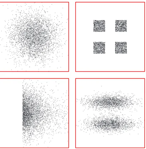
FIGURE 10.6. These four data sets have identical statistics up to second-order—that is, the same mean ! and covariance ". In such cases it is important to include in the
model more parameters to represent the structure more completely. From: Richard O. Duda, Peter E. Hart, and David G. Stork, Pattern Classification. Copyright c! 2001 by John Wiley & Sons, Inc.
Steps for Clustering
1. Feature Selection
•
Ideal: small number of features with little redundancy2. Similarity (or Proximity) Measure
•
Measure of similarity or dissimilarity3. Clustering Criterion
•
Determine how distance patterns determine cluster likelihood (e.g. preferring circular to elongated clusters)4. Clustering Algorithm
•
Search method used with the clustering criterion to identify clusters5. Validation of Results
•
Using appropriate tests (e.g. statistical)6. Interpretation of Results
•
Domain expert interprets clusters (clusters are subjective) 7Red: defining ‘cluster space’
Choosing a Similarity Measure
Most Common: Euclidean Distance
Roughly speaking, want distance between samples in a cluster to be smaller than the distance between samples in different clusters
•
Example (next slide): define clusters by a maximum distance d0 between a point and a point in a cluster•
Rescaling features can be useful (transform the space)•
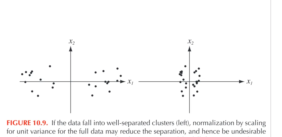
Unfortunately, normalizing data (e.g. by settingfeatures to zero mean, unit variance) may eliminate subclasses
•
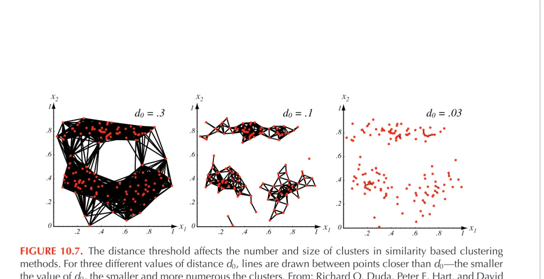
One might also choose to rotate axes so they coincide with eigenvectors of the covariance matrix (i.e. apply PCA).2 .4 .6 .8 1 0 .2 .4 .6 .8 1 .2 .4 .6 .8 1 0 .2 .4 .6 .8 .2 .4 .6 .8 1 0 .2 .4 .6 .8 1 d0 = .3 x1 x1 x1 x2 x2 x2 1 d0 = .1 d0 = .03
FIGURE 10.7. The distance threshold affects the number and size of clusters in similarity based clustering methods. For three different values of distanced0, lines are drawn between points closer thand0—the smaller
the value ofd0, the smaller and more numerous the clusters. From: Richard O. Duda, Peter E. Hart, and David
.2 .4 .6 .8 1 0 .2 .4 .6 .8 1 .25 .5 .75 1 1.25 1.5 1.75 2 0 .1 .2 .3 .4 .5 .1 .2 .3 .4 .5 0 .2 .4 .6 .8 1 1.2 1.4 1.6 2 0 0 .5
( )
x2 x2 x2 x1 x1 x1 .5 0 0 2( )
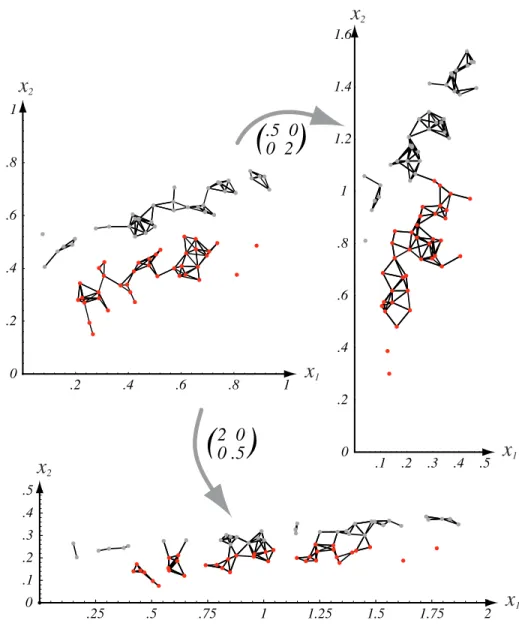
FIGURE 10.8. Scaling axes affects the clusters in a minimum distance cluster method. The original data and minimum-distance clusters are shown in the upper left; points in one cluster are shown in red, while the others are shown in gray. When the vertical axis is expanded by a factor of 2.0 and the horizontal axis shrunk by a factor of 0.5, the clustering is altered (as shown at the right). Alternatively, if the vertical axis is shrunk by a factor of 0.5 and the horizontal axis is expanded by a factor of 2.0, smaller more nu-merous clusters result (shown at the bottom). In both these scaled cases, the assignment of points to clusters differ from that in the original space. From: Richard O. Duda, Peter E. Hart, and David G. Stork, Pattern Classification. Copyright c! 2001 by John Wiley & Sons, Inc.
x1 x1
x2 x2
FIGURE 10.9. If the data fall into well-separated clusters (left), normalization by scaling for unit variance for the full data may reduce the separation, and hence be undesirable (right). Such a normalization may in fact be appropriate if the full data set arises from a single fundamental process (with noise), but inappropriate if there are several different processes, as shown here. From: Richard O. Duda, Peter E. Hart, and David G. Stork, Pattern Classification. Copyright c! 2001 by John Wiley & Sons, Inc.
Other Similarity Measures
Minkowski Metric (
Dissimilarity)
Change the exponent q:
•
q = 1: Manhattan (city-block) distance•
q = 2: Euclidean distance (only form invariant to translation and rotation in feature space)Cosine
Similarity
Characterizes
similarity
by the cosine of the angle
between two feature vectors (in [0,1])
•
Ratio of inner product to vector magnitude product•
Invariant to rotations and dilation (not translation) 12 d(x,x!) = ! d " k=1 |xk − x!k|q #1/q 1 d(x,x!) = ! d " k=1 |xk − x!k|q #1/q s(x,x!) = x Tx! ||x|| ||x!|| 1More on Cosine Similarity
If features binary-valued:
•
Inner product is sum of shared feature values
•
Product of magnitudes is geometric mean of
number of attributes in the two vectors
Variations
Frequently used for Information Retrieval
•
Ratio of shared attributes (identical lengths):
•
Tanimoto distance
: ratio of shared attributes to
attributes in x or x’
13 d(x,x!) = ! d " k=1 |xk − x!k|q #1/q s(x,x!) = x Tx! ||x|| ||x!|| s(x,x!) = x Tx! d s(x,x!) = x Tx! xTx + x!Tx! − xTx! 1 d(x,x!) = ! d " k=1 |xk − x!k|q #1/q s(x,x!) = x Tx! ||x|| ||x!|| s(x,x!) = x Tx! d s(x,x!) = x Tx! xTx + x!Tx! − xTx! 1 d(x,x!) = ! d " k=1 |xk − x!k|q #1/q s(x,x!) = x Tx! ||x|| ||x!|| 1Cosine Similarity: Tag Sets for YouTube
Videos (Example by K. Kluever)
Let A and B be binary vectors of the same
length (represent all tags in A&B)
14
While there are often additional words to be obtained from
a video’s title [7], in our preliminary user study we found
that adding titles did not substantially increase the usability
of the system (e.g. we observed a decrease in security of 5%
and only an increase in usability of 0.3% relative to matching
against only author-supplied tags). In addition, we could not
estimate the security impact of adding title words using our
tag frequencies (which are calculated over tag space, not title
space), and so we decided to not allow title words.
Sorting Related Videos by Cosine Similarity
To select tags from those videos that have the most similar
tag set to the challenge video, we performed a sort using
the
cosine similarity
of the tags on related videos and the
tags on the challenge video. The cosine similarity metric is
a standard similarity metric used in
Information Retrieval
to
compare text documents [20]. The cosine similarity between
two vectors
A
and
B
can be easily computed as follows:
S
IM(
A, B
) = cos
θ
=
A
·
B
!
A
!!
B
!
The dot product and product of magnitudes are:
A
·
B
=
n!
i=1a
ib
i!
A
!!
B
!
=
"
#
#
$
n!
i=1(
a
i)
2"
#
#
$
n!
i=1(
b
i)
2In our case,
A
and
B
are binary
tag occurrences vectors
(i.e.,
they only contain 1’s and 0’s) over the union of the tags in
both videos. Therefore, the dot product simply reduces to
the size intersection of the two tag sets (i.e.,
|
A
t∩
R
t|
) and
the product of the magnitudes reduces to the square root of
the number of tags in the first tag set times the square root of
the number of tags in the second tag set (i.e.,
%
|
A
t|
%
|
R
t|
).
Therefore, the cosine similarity between a set of author tags
and a set of related tags can easily be computed as:
cos
θ
=
%
|
A
t∩
R
t|
|
A
t|
%
|
R
t|
Tag Set Occ. Vector dog puppy funny cat
A
tA
1
1
1
0
R
tB
1
1
0
1
Table 1. Example of a tag occurrence table.
Consider an example where
A
t=
{
dog, puppy, f unny
}
and
R
t=
{
dog, puppy, cat
}
. We can build a simple
ta-ble which corresponds to the tag occurrence over the union
of both tag sets (see Table 1). Reading row-wise from this
table, the tag occurrence vectors for
A
tand
R
tare
A
=
{
1
,
1
,
1
,
0
}
and
B
=
{
1
,
1
,
0
,
1
}
, respectively. Next, we
compute the dot product:
A
·
B
= (1
∗
1) + (1
∗
1) + (1
∗
0) + (0
∗
1) = 2
The product of the magnitudes can also easily be computed:
!
A
!!
B
!
=
√
3
√
3 = 3
Thus, the cosine similarity of the two videos is
23
= 0
.
¯6
.
Adding Related Tags
Once the related videos are sorted in decreasing cosine
sim-ilarity order, we introduce tags from the related videos into
the ground truth. The maximum number of characters
al-lowed in a YouTube tag set is 120. In the worst case, the
tag set could contain 60 unique words (each word would
be a single character), separated by spaces. The maximum
number of related videos which YouTube provides is 100.
Therefore, adding all of the related tags could potentially
add up to 6000 new tags. We chose to limit the upper bound
by adding up to
n
additional unique tags from the related
videos (sorted in decreasing cosine similarity order). Given
a challenge video
v
, a set of related videos
R
, and a
num-ber of related tags to generated
n
, the following algorithm
generates up to
n
related tags.
R
ELATEDT
AGS(
A, R, n
)
1. Create an empty set,
Z
← ∅
.
2. Sort related videos
R
in decreasing cosine similarity order
of their tag sets relative to the tag set
A
(for a challenge
video
v
).
3. For each related video
r
∈
R
:
(a) If the number of new tags on the related video
r
is
≤
n
−
|
Z
|
, add them all to
Z
.
(b) Otherwise, while the related video
r
has tags and
while
|
Z
|
< n
:
i. Randomly remove a tag from the remaining tags
on the related video
r
, and add this tag to
Z
.
4. Return
Z
.
This technique will introduce up to
n
additional tags to the
ground truth set. In the case where we have already
gener-ated
n
−
b
related tags and the next related video contains
more than
b
new, unique tags, we cannot add all of them
without exceeding our upper bound of
n
tags. For example,
consider the case in which we wish to generate 100
addi-tional tags (
n
= 100
) and we have already generated 99 tags.
If the next related video has 4 new tags, we cannot include
all of these in the new tag set, and so we randomly pick one
to avoid bias.
Rejecting Frequent Tags
Security against
frequency-based attacks
(an attack where
the three most frequent tags are always submitted) is
main-tained through the parameters
F
and
t
in the challenge
gen-erating function V
IDEOC
APTCHA(see earlier in this
sec-tion).
F
is a tag frequency distribution (see Figure 2) and
t
is a frequency rejection threshold. During challenge
gener-ation, after author-supplied tags and tags from related videos
have been added to the ground-truth set, tags with a
fre-quency greater than or equal to
t
in
F
are removed.
R
EJECTF
REQUENTT
AGS(
S
,
F
,
t
)
4
While there are often additional words to be obtained from a video’s title [7], in our preliminary user study we found that adding titles did not substantially increase the usability of the system (e.g. we observed a decrease in security of 5% and only an increase in usability of 0.3% relative to matching against only author-supplied tags). In addition, we could not estimate the security impact of adding title words using our tag frequencies (which are calculated over tag space, not title space), and so we decided to not allow title words.
Sorting Related Videos by Cosine Similarity
To select tags from those videos that have the most similar tag set to the challenge video, we performed a sort using the cosine similarity of the tags on related videos and the tags on the challenge video. The cosine similarity metric is a standard similarity metric used in Information Retrieval to compare text documents [20]. The cosine similarity between two vectors A and B can be easily computed as follows:
SIM(A, B) = cos θ = A · B !A!!B!
The dot product and product of magnitudes are:
A · B = n ! i=1 aibi !A!!B! = " # # $ n ! i=1 (ai)2 " # # $ n ! i=1 (bi)2
In our case, A and B are binary tag occurrences vectors (i.e.,
they only contain 1’s and 0’s) over the union of the tags in both videos. Therefore, the dot product simply reduces to the size intersection of the two tag sets (i.e., |At ∩ Rt|) and
the product of the magnitudes reduces to the square root of the number of tags in the first tag set times the square root of the number of tags in the second tag set (i.e., %|At|%|Rt|).
Therefore, the cosine similarity between a set of author tags and a set of related tags can easily be computed as:
cosθ = %|At ∩ Rt| |At|%|Rt|
Tag Set Occ. Vector dog puppy funny cat
At A 1 1 1 0
Rt B 1 1 0 1
Table 1. Example of a tag occurrence table.
Consider an example where At = {dog, puppy, f unny}
and Rt = {dog, puppy, cat}. We can build a simple
ta-ble which corresponds to the tag occurrence over the union of both tag sets (see Table 1). Reading row-wise from this table, the tag occurrence vectors for At and Rt are A =
{1,1, 1,0} and B = {1,1, 0,1}, respectively. Next, we
compute the dot product:
A · B = (1 ∗ 1) + (1 ∗ 1) + (1 ∗ 0) + (0 ∗ 1) = 2
The product of the magnitudes can also easily be computed:
!A!!B! = √3√3 = 3
Thus, the cosine similarity of the two videos is 2
3 = 0.¯6.
Adding Related Tags
Once the related videos are sorted in decreasing cosine sim-ilarity order, we introduce tags from the related videos into the ground truth. The maximum number of characters al-lowed in a YouTube tag set is 120. In the worst case, the tag set could contain 60 unique words (each word would be a single character), separated by spaces. The maximum number of related videos which YouTube provides is 100. Therefore, adding all of the related tags could potentially add up to 6000 new tags. We chose to limit the upper bound by adding up to n additional unique tags from the related
videos (sorted in decreasing cosine similarity order). Given a challenge video v, a set of related videos R, and a
num-ber of related tags to generated n, the following algorithm
generates up to n related tags.
RELATEDTAGS(A, R, n)
1. Create an empty set, Z ← ∅.
2. Sort related videos R in decreasing cosine similarity order
of their tag sets relative to the tag set A (for a challenge
video v).
3. For each related video r ∈ R:
(a) If the number of new tags on the related video r is ≤ n − |Z|, add them all to Z.
(b) Otherwise, while the related video r has tags and
while |Z| < n:
i. Randomly remove a tag from the remaining tags on the related video r, and add this tag to Z.
4. Return Z.
This technique will introduce up to n additional tags to the
ground truth set. In the case where we have already gener-ated n − b related tags and the next related video contains
more than b new, unique tags, we cannot add all of them
without exceeding our upper bound of n tags. For example,
consider the case in which we wish to generate 100 addi-tional tags (n = 100) and we have already generated 99 tags.
If the next related video has 4 new tags, we cannot include all of these in the new tag set, and so we randomly pick one to avoid bias.
Rejecting Frequent Tags
Security against frequency-based attacks (an attack where the three most frequent tags are always submitted) is main-tained through the parameters F and t in the challenge
gen-erating function VIDEOCAPTCHA (see earlier in this
sec-tion). F is a tag frequency distribution (see Figure 2) and t is a frequency rejection threshold. During challenge
gener-ation, after author-supplied tags and tags from related videos have been added to the ground-truth set, tags with a fre-quency greater than or equal to t in F are removed.
REJECTFREQUENTTAGS(S, F, t)
4
Additional Similarity Metrics
Theodoridis Text
Defines a
large
number of alternative
distance metrics, including:
•
Hamming distance: number of locations where
two vectors (usually bit vectors) disagree
•
Correlation coefficient
•
Weighted distances...
Criterion Functions for Clustering
Criterion Function
Quantifies ‘quality’ of a set of clusters
•
Clustering task
: partition data set
D
into
c
disjoint
sets D
1... D
c•
Choose partition maximizing the criterion function
d
(
x
,
x
!) =
! d " k=1|
x
k−
x
!k|
q #1/qs
(
x
,
x
!) =
x
Tx
!||
x
|| ||
x
!||
s
(
x
,
x
!) =
x
Tx
!d
s
(
x
,
x
!) =
x
Tx
!x
Tx
+
x
!Tx
!−
x
Tx
!J
e=
c " i=1 " x∈Di||
x
−
µ
Di||
21
Criterion: Sum of Squared Error
Measures total squared ‘error’ incurred by choice of
cluster centers (cluster means)
‘Optimal’ Clustering
Minimizes
this quantity
Issues
•
Well suited when clusters compact and well-separated•
Different # points in each cluster can lead to large clusters being split ‘unnaturally’ (next slide)Je= large
Je= small
FIGURE 10.10. When two natural groupings have very different numbers of points, the
clusters minimizing a sum-squared-error criterion Je of Eq. 54 may not reveal the true
underlying structure. Here the criterion is smaller for the two clusters at the bottom than for the more natural clustering at the top. From: Richard O. Duda, Peter E. Hart, and
Related Criteria: Min Variance
An Equivalent Formulation for SSE
: mean squared distance between points in cluster i
(variance)
•
Alternative Criterions:
use median, maximum, other
descriptive statistic on distance for
Variation: Using Similarity (e.g. Tanimoto)
s
may be any similarity function (in this case,
maximize)
19 Je = 1 2 c ! i=1 nis¯i ¯ si = 1 n2 i ! x∈Di ! x!∈Di ||x − x"||2 2
J
e=
1
2
c!
i=1n
is
¯
i¯
s
i=
1
n
2i!
x∈Di!
x!∈Di||
x
−
x
"||
2¯
s
i=
1
n
2i!
x∈Di!
x!∈Dis
(
x
,
x
")
¯
s
i= min
x,x!∈Dis
(
x, x
")
2
J
e=
1
2
c ! i=1n
is
¯
i¯
s
i=
1
n
2i ! x∈Di ! x!∈Di||
x
−
x
"||
2¯
s
i=
1
n
2i ! x∈Di ! x!∈Dis
(
x
,
x
")
¯
s
i= min
x,x!∈Dis
(
x, x
")
2
J
e=
1
2
c ! i=1n
is
¯
i¯
s
i=
1
n
2i ! x∈Di ! x!∈Di||
x
−
x
"||
2¯
s
i=
1
n
2i ! x∈Di ! x!∈Dis
(
x
,
x
")
¯
s
i= min
x,x!∈Dis
(
x, x
")
2
J
e=
1
2
c ! i=1n
is
¯
i¯
s
i=
1
n
2i ! x∈Di ! x!∈Di||
x
−
x
"||
2¯
s
i=
1
n
2i ! x∈Di ! x!∈Dis
(
x
,
x
")
¯
s
i= min
x,x!∈Dis
(
x, x
")
2
Je = 1 2 c ! i=1 nis¯i ¯ si = 1 n2i ! x∈Di ! x!∈Di ||x − x"||2 2Criterion: Scatter Matrix-Based
Minimize Trace of S
w(within-class)
Equivalent to SSE!
Recall that total scatter is the sum of within
and between-class scatter (Sm = Sw + Sb).
This means that by minimizing the trace of
Sw, we also maximize Sb (
as Sm is fixed
):
20 Sw = c ! i=1 ! x∈Di (x − µi)(x − µi)T trace[Sw] = c ! i=1 trace[Si] = c ! i=1 ! x∈Di ||x − µi||2 = Je 3
S
w=
c ! i=1 ! x∈Di(
x
−
µ
i)(
x
−
µ
i)
Ttrace
[
S
w] =
c ! i=1 ! x∈Di||
x
−
µ
i||
2=
J
e3
S
w=
c ! i=1 ! x∈Di(
x
−
µ
i)(
x
−
µ
i)
Ttrace
[
S
w] =
c ! i=1 ! x∈Di||
x
−
µ
i||
2=
J
etrace
[
S
b] =
c ! i=1n
i||
µ
i−
µ
0||
23
Scatter-Based Criterions, Cont’d
Determinant Criterion
Roughly measures square of the scattering
volume; proportional to product of variances
in principal axes (
minimize!)
•
Minimum error partition will not change with
axis scaling, unlike SSE
21 Sw = c ! i=1 ! x∈Di (x − µi)(x − µi)T trace[Sw] = c ! i=1 ! x∈Di ||x − µi||2 = Je trace[Sb] = c ! i=1 ni||µi − µ0||2 Jd = |Sw| = " " " " " " c ! i=1 ! x∈Di (x − µi)(x − µi)T " " " " " " 3
Scatter-Based: Invariant Criteria
Invariant Criteria (Eigenvalue-based)
Eigenvalues: measure ratio of between to
within-cluster scatter in direction of eigenvectors
(
maximize!)
•
Trace of a matrix is sum of eigenvalues (here
d
is
length of feature vector)
•
Eigenvalues are
invariant
under non-singular linear
transformations (rotations, translations, scaling, etc.)
22
S
w=
c ! i=1 ! x∈Di(
x
−
µ
i)(
x
−
µ
i)
Ttrace
[
S
w] =
c ! i=1 ! x∈Di||
x
−
µ
i||
2=
J
etrace
[
S
b] =
c ! i=1n
i||
µ
i−
µ
0||
2J
d=
|
S
w|
=
" " " " " " c ! i=1 ! x∈Di(
x
−
µ
i)(
x
−
µ
i)
T " " " " " "trace
[
S
w−1S
b] =
d ! i=1λ
i3
Sw = c ! i=1 ! x∈Di (x − µi)(x − µi)T trace[Sw] = c ! i=1 ! x∈Di ||x − µi||2 = Je trace[Sb] = c ! i=1 ni||µi − µ0||2 Jd = |Sw| = " " " " " " c ! i=1 ! x∈Di (x − µi)(x − µi)T " " " " " " trace[Sw−1Sb] = d ! i=1 λi Jf = trace[Sm−1Sw] = d ! i=1 1 1 + λi 3Clustering with a Criterion
Choosing Criterion
Creates a well-defined problem
•
Define clusters so as to maximize the
criterion function
•
A search problem
•
Brute force solution:
enumerate partitions
of the training set, select the partition with
maximum criterion value
Comparison: Scatter-Based Criteria
Hierarchical Clustering
Motivation
Capture similarity/distance relationships
between sub-groups and samples
within
the
chosen clusters
•
Common in scientific taxonomies (e.g.
biology)
•
Can operate bottom up (individual samples to
clusters, or
agglomerative
clustering) or
top-down (single cluster to individual samples, or
divisive
clustering)
Agglomerative Hierarchical Clustering
Problem: Given n samples, we want c clusters
One solution: Create a sequence of partitions (clusterings)
•
First partition, k = 1: n clusters (one cluster per sample)•
Second partition, k = 2: n-1 clusters•
Continue reducing the number of clusters by one: merge 2 closestclusters (a cluster may be a single sample) at each step k until...
•
Goal partition: k = n - c + 1: c clusters•
Done; but if we’re curious, we can continue on until the...•
....Final partition, k = n: one clusterResult
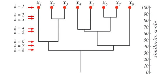
All samples and sub-clusters organized into a tree (a dendrogram)
•
Often show cluster similarity for a dendrogram diagram (Y-axis) If as stated above whenever two samples share a cluster they remain inx1 x2 x3 x4 x5 x6 x7 x8 k = 8 7 6 5 3 4 2
FIGURE 10.12. A set or Venn diagram representation of two-dimensional data (which was used in the dendrogram of Fig. 10.11) reveals the hierarchical structure but not the quantitative distances between clusters. The levels are numbered by k, in red. From: Richard O. Duda, Peter E. Hart, and David G. Stork, Pattern Classification. Copyright
c
! 2001 by John Wiley & Sons, Inc.
0 10 20 30 40 50 60 70 80 90 100 x1 similarity scale k = 1 k = 2 k = 3 k = 4 k = 5 k = 6 k = 7 x2 x3 x4 x5 x6 x7 x8 k = 8
FIGURE 10.11. A dendrogram can represent the results of hierarchical clustering algo-rithms. The vertical axis shows a generalized measure of similarity among clusters. Here, at level 1 all eight points lie in singleton clusters; each point in a cluster is highly similar to itself, of course. Points x6 andx7 happen to be the most similar, and are merged at
level 2, and so forth. From: Richard O. Duda, Peter E. Hart, and David G. Stork,Pattern Classification. Copyright c!2001 by John Wiley & Sons, Inc.
Distance Measures
Listed Above:
Minimum, maximum and average inter-sample
distance (samples for clusters i,j: D
i, D
j)
Difference in cluster means (m
i, m
j)
28 dmin(Di, Dj) = min x∈Di,x∈Dj || x − x"|| dmax(Di, Dj) = max x∈Di,x∈Dj || x −x"|| davg(Di, Dj) = 1 ninj ! x∈Di ! x!∈Dj ||x −x"|| dmean(Di, Dj) = ||mi − mj|| 5
Nearest-Neighbor Algorithm
Also Known as “Single-Linkage” Algorithm
Agglomerative hierarchical clustering using dmin
•
Two nearest neighbors in separate clusters determine clusters merged at each step•
If we continue until k = n (c = 1), produce a minimum spanning tree(similar to Kruskal’s alg.)
•
MST: Path exists between all node (sample) pairs, sum of edge costs minimum for all spanning treesIssues
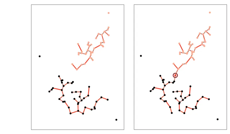
Sensitive to noise and slight changes in position of data points (chaining effect)
•
Example: next slide29 dmin(Di, Dj) = min x∈Di,x∈Dj || x − x"|| dmax(Di, Dj) = max x∈Di,x∈Dj || x − x"|| davg(Di, Dj) = 1 ninj ! x∈Di ! x!∈Dj ||x − x"|| dmean(Di, Dj) = ||mi − mj|| 5
FIGURE 10.13. Two Gaussians were used to generate two-dimensional samples, shown in pink and black. The nearest-neighbor clustering algorithm gives two clusters that well approximate the generating Gaussians (left). If, however, another particular sample is generated (circled red point at the right) and the procedure is restarted, the clusters do not well approximate the Gaussians. This illustrates how the algorithm is sensitive to the details of the samples. From: Richard O. Duda, Peter E. Hart, and David G. Stork,
d
min(
D
i, D
j) =
min
x∈Di,x∈Dj||
x
−
x
"||
d
max(
D
i, D
j) =
max
x∈Di,x∈Dj||
x
−
x
"||
d
avg(
D
i, D
j) =
1
n
in
j ! x∈Di ! x!∈Dj||
x
−
x
"||
d
mean(
D
i, D
j) =
||
m
i−
m
j||
5
Farthest-Neighbor Algorithm
Agglomerative hierarchical clustering using d
max•
Clusters with the smallest maximum distance between two points are merged at each step•
Goal: minimal increase to largest cluster diameter at each iteration (discourages elongated clusters)•
Known as ‘Complete-Linkage Algorithm’ if terminated when distance between nearest clusters exceeds a given threshold distanceIssues
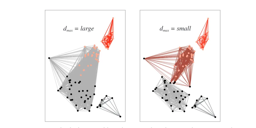
Works well for compact and roughly equal in size; with
dmax = large dmax = small
FIGURE 10.14. The farthest-neighbor clustering algorithm uses the separation between the most distant points as a criterion for cluster membership. If this distance is set very large, then all points lie in the same cluster. In the case shown at the left, a fairly large dmax leads to three clusters; a smallerdmax gives four clusters, as shown at the right. From:
Richard O. Duda, Peter E. Hart, and David G. Stork, Pattern Classification. Copyright c
dmin(Di, Dj) = min x∈Di,x∈Dj || x − x"|| dmax(Di, Dj) = max x∈Di,x∈Dj || x − x"|| davg(Di, Dj) = 1 ninj ! x∈Di ! x!∈Dj ||x − x"|| dmean(Di, Dj) = ||mi −mj|| 5
Using Mean, Avg Distances
Reduces Sensitivity to Outliers
Mean less expensive to compute than avg,
min, max (each require n
i* n
jdistances)
Stepwise Optimal Hierarchical Clustering
Problem
None of the agglomerative methods discussed so far directly
minimize a specific criterion function
Modified Agglomerative Algorithm:
For k = 1 to (n - c + 1)
•
Find clusters whose merger changes criterion least, Di and Dj•
Merge Di and DjExample: Minimal increase in SSE (Je)
de defines the cluster pair that increases Je as little as possible. May not
minimize SSE, but often good starting point
•
prefers merging single elements or small with large clusters vs.merging medium-size clusters 34
dmin(Di, Dj) = min x∈Di,x∈Dj ||x − x "|| dmax(Di, Dj) = max x∈Di,x∈Dj || x − x"|| davg(Di, Dj) = 1 ninj ! x∈Di ! x!∈Dj ||x − x"|| dmean(Di, Dj) = ||mi − mj|| de(Di, Dj) = " ninj ni + nj|| mi − mj|| 5
k-Means Clustering
k-Means Algorithm
For a number of clusters k:
1. Choose k data points at random
2. Assign all data points to closest of the k cluster centers
3. Re-compute k cluster centers as the mean vector of each cluster
•
If cluster centers do not change, stop•
Else, goto 2Complexity
O(ndcT) - T iterations, d features, n points, c clusters, in practice usually T << n (much fewer than n iterations)
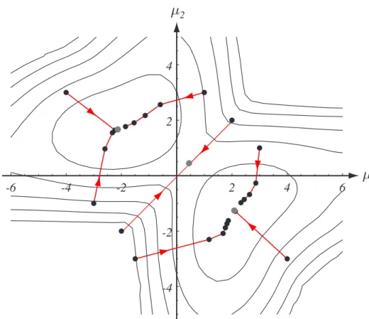
-6 -4 -2 2 4 6 -4 -2 2 4 µ1 µ2
FIGURE 10.2. The k-means clustering procedure is a form of stochastic hill climbing in the log-likelihood function. The contours represent equal log-likelihood values for the one-dimensional data in Fig. 10.1. The dots indicate parameter values after different iterations of the k-means algorithm. Six of the starting points shown lead to local max-ima, whereas two (i.e.,µ1(0) = µ2(0)) lead to a saddle point near ! = 0. From: Richard
O. Duda, Peter E. Hart, and David G. Stork, Pattern Classification. Copyright c! 2001 by John Wiley & Sons, Inc.
-5 -2.5 0 2.5 5 -4 -2 0 2 4 -150 -100 -50 -4 -3 -2 -1 0 1 2 3 4 x source density l(µ1, µ2) µ1 µ2 -56.7 -52.2 µ a µb p(x|µb) p(x|µa) start start
FIGURE 10.1. (Above) The source mixture density used to generate sample data, and two maximum-likelihood estimates based on the data in the table. (Bottom) Log-likelihood of a mixture model consisting of two univariate Gaussians as a function of their means, for the data in the table. Trajectories for the iterative maximum-likelihood estimation of the means of a two-Gaussian mixture model based on the data are shown as red lines. Two local optima (with log-likelihoods−52.2 and−56.7) correspond to the
two density estimates shown above. From: Richard O. Duda, Peter E. Hart, and David G. Stork,Pattern Classification. Copyright c"2001 by John Wiley & Sons, Inc.
x1
x2
1 3 2
FIGURE 10.3. Trajectories for the means of the k-means clustering procedure applied to two-dimensional data. The final Voronoi tesselation (for classification) is also shown— the means correspond to the “centers” of the Voronoi cells. In this case, convergence is obtained in three iterations. From: Richard O. Duda, Peter E. Hart, and David G. Stork, Pattern Classification. Copyright c! 2001 by John Wiley & Sons, Inc.
Fuzzy k-means
Basic Idea
Allow every point to have a probability of
membership in every cluster. The criterion (cost
function) minimized is:
Theta is the membership function parameter set.
b
(‘blending’) is a free parameter:
•
b = 0: Sum of squared error criterion (one cluster per data point)•
b > 1: each pattern may belong to multiple clusters 39Jf uz = c ! i=1 n ! j=1 [ ˆP(ωi|xj, Θ)]ˆ b||xj − µi||2 6
Fuzzy k-Mean Clustering Algorithm
Algorithm
1. Compute probability of each class for every point in the training set (uniform probability: equal likelihood in each cluster)
2. Recompute means using expression at top-left
3. Recompute probability of each class for each point using expression at top right
•
If change in means and membership probabilities for points is small, stop•
Else goto 2 40J
f uz=
c ! i=1 n ! j=1[ ˆ
P
(
ω
i|
x
j,
Θ
ˆ
)]
b||
x
j−
µ
i||
2µ
j=
"n j=1[ ˆ
P
(
ω
i|
x
j)]
bx
j "n j=1[ ˆ
P
(
ω
i|
x
j)]
b6
Jf uz = c ! i=1 n ! j=1 [ ˆP(ωi|xj,Θˆ)]b||xj − µi||2 µj = "n j=1[ ˆP(ωi|xj)]bxj "n j=1[ ˆP(ωi|xj)]b ˆ P(ωi|xj) = (1/dij) 1/(b−1) "c r=1(1/drj)1/(b−1) dij = ||xj − µi||2 6x1 x2 1 2 3 4
FIGURE 10.4. At each iteration of the fuzzy k-means clustering algorithm, the prob-ability of category memberships for each point are adjusted according to Eqs. 32 and 33 (here b = 2). While most points have nonnegligible memberships in two or three clusters, we nevertheless draw the boundary of a Voronoi tesselation to illustrate the progress of the algorithm. After four iterations, the algorithm has converged to the red cluster centers and associated Voronoi tesselation. From: Richard O. Duda, Peter E. Hart, and David G. Stork, Pattern Classification. Copyright c! 2001 by John Wiley & Sons, Inc.