Statistical Techniques for Online Anomaly Detection in Data Centers

Keyword(s):

Abstract:

Statistical Techniques for Online Anomaly Detection in Data Centers

Chengwei Wang, Krishnamurthy Viswanathan, Lakshminarayan Choudur, Vanish Talwar, Wade

Satterfield, Karsten Schwan

HP Laboratories

HPL-2011-8

Anomaly Detection, Data Center Management, Statistics, Algorithms

Online anomaly detection is an important step in data center management, requiring light-weight

techniques that provide sufficient accuracy for subsequent diagnosis and management actions. This paper

presents statistical techniques based on the Tukey and Relative Entropy statistics, and applies them to data

collected from a production environment and to data captured from a testbed for multi-tier web applications

running on server class machines. The proposed techniques are lightweight and improve over standard

Gaussian assumptions in terms of performance.

External Posting Date: May 21, 2011 [Fulltext] Approved for External Publication Internal Posting Date: May 21, 2011 [Fulltext]

To be published and presented at IFIP/IEEE International Symposium on Integrated Network Management (1M) 2011, 23 May - 27 May 2011

Statistical Techniques for Online Anomaly

Detection in Data Centers

Chengwei Wang, Krishnamurthy Viswanathan*, Lakshminarayan Choudur*, Vanish Talwar*,

Wade Satterfield*, Karsten Schwan

CERCS, Georgia Institute of Technology

{flinter,schwan}@cc.gatech.edu

*Hewlett-Packard

{krishnamurthy.viswanathan,choudur.lakshminarayan,vanish.talwar,wade.satterfield}@hp.com

Abstract—Online anomaly detection is an important step in data center management, requiring light-weight techniques that provide sufficient accuracy for subsequent diagnosis and management actions. This paper presents statistical techniques based on the Tukey and Relative Entropy statistics, and applies them to data collected from a production environment and to data captured from a testbed for multi-tier web applications running on server class machines. The proposed techniques are lightweight and improve over standard Gaussian assumptions in terms of performance.

I. INTRODUCTION

Commercial data center environments are increasingly char-acterized by extremely large scale and complexity. Individual applications like Hadoop MapReduce and Web 2.0 can involve thousands of servers. Utility clouds like Amazon EC2 or Google App are able to serve more than 2 millions businesses to run their own applications, each of which may have dif-ferent workload characteristics. These facts make data center management a difficult task, especially in systems where malfunctions can lead to extensive losses in profit due to lack of responsiveness or availability.

Our work seeks to improve system performance and avail-ability by developing online, closed loop management solu-tions that (i) detect problems, (ii) diagnose them to determine potential remedies or mitigation methods, and (iii) trigger and carry out such solutions. A key element of such research and the topic of this paper is online anomaly detection, which is to understand whether a system is behaving as expected or whether it is behaving in ways that are unusual and deserve further investigation and diagnosis. Anomaly detection is important because it must be done continuously, as long as a system is running and at scale – for entire data center systems. We are interested in online anomaly detection solutions that can be applied to continuous monitoring scenarios as opposed to methods that rely on static profiling or limited sets of historical data. There are several challenges in designing effective solutions for such online anomaly detection in large data centers. These include scale, for which the anomaly detection methods must be ‘lightweight’, both in terms of the number of metrics they require to run (the volume of moni-toring data continuously captured and used), and in terms of their runtime complexity for executing the detection methods.

Next, these methods should have the ability to handle multiple metrics at the different levels of abstraction – hardware, system software, middleware, or applications – present in data centers. Furthermore, the methods need to accommodate the workload characteristics and patterns including day of the week, and hour of the day patterns of workload behavior. The methods also need to be aware of and address the dynamic nature of data center systems and applications, including dealing with application arrivals and departures, changes in workload, and system-level load balancing through say, virtual machine migration. Finally, the solutions must exhibit good accuracy and low false alarm for meaningful results.

The state of the art approaches for anomaly detection deployed in today’s data centers apply a fixed threshold on the metrics being monitored. These thresholds are usually com-puted offline from training data and remain constant during the entire process of anomaly detection. Often these thresholds are applied to each individual measurement separately. Variants such as Multivariate Adaptive Statistical Filtering (MASF) [1] additionally maintain a separate threshold for data segmented and aggregated by time (e.g., hour of day, day of week). How-ever, these existing techniques assume the data distribution to be Gaussian for determining the threshold values. This assumption is frequently violated in practice. Furthermore, fixed thresholds cannot adapt to loads that may change over time or intermittent bursts, nor can they react to anomalous behavior that may not show up as extremal large or small values in the data. All of these lead to false alarms and reduced accuracy with existing techniques.

We propose statistical techniques in this paper that over-come these limitations improving accuracy and insights raised by anomaly flags. We make the following contributions:

∙ We select two statistical techniques, Tukey method and the multinomial goodness-of-fit test based on theRelative

Entropy statistic, and adapt them to the specific needs

for anomaly detection in data centers. Algorithms using these techniques are proposed that compute statistics on data based on multiple time dimensions - entire past, recent past, and context based on hour of day and day of week. These statistics are then employed to determine if specific points or windows are anomalies. The proposed algorithms have low complexity and are scalable to

process large amounts of data.

∙ We have experimented the proposed algorithms with data from a 3-tier RUBis (Internet Service) testbed with injected performance and configuration anomalies, as well as data from production testbeds. Our results have shown improvement in accuracy and reduction in false alarm rates compared to state of art Gaussian techniques. Further, our techniques are shown to be more adaptable to varying workload changes and they learn the multiple states of operation of the workload over time. Further-more, we also illustrate how results from multiple time dimensions and multiple techniques can be combined to provide improved insights on application behavior to administrators.

The remainder of this paper is organized as follows. Sec-tion II provides background informaSec-tion on existing niques. Section III describes our proposed statistical tech-niques that overcome limitations of existing approaches. Ex-perimental results are presented in Section IV. Section V provides discussion on combining results from multiple time dimensions. Section VI discusses related work, and we finally conclude the paper in Section VII.

II. BACKGROUND

Anomalies manifest in data in a variety of ways. Two common manifestations are those in which a data point is atypical with reference to the normal behavior of the data distribution, and secondly those when the distribution of the data changes with time. One way of dealing with the first

problem is to use the distribution of the data to compute thresholds. Typical data under normal process behavior will oscillate within the threshold limits. Data points falling beyond and below the upper and lower thresholds respectively are flagged as anomalies. These thresholds are obtained under cer-tain assumptions about the behavior (shape) of the distribution. An understanding and quantitative representation of the data distribution is obtained by studying the historical data. This approach is known as parametric thresholding. To address the

secondproblem, the variability in the process over an extended period of time is studied and analyzed by using the historical repository of data. From this, an estimate of the variability of the data is characterized and threshold limits are computed. This approach avoids the necessity to make assumptions about the shape of the distribution of the data. Such methods are known as non-parametric methods.

In many applications involving statistical analysis of data, the Gaussian distribution is the assumed underlying probability model [10]. For example, a popular method for anomaly detection in data centers is MASF [1] which relies on the Gaussian law. MASF first segments the data by hour of day and day of week. Subsequently, threshold limits are computed based on the standard deviation (𝜎) of this segregated data. Under Gaussian assumptions, 95% of the data is within the 2 standard deviations (𝜎) of the mean (𝜇), and 99 % of the data is within 3 standard deviations of the mean 𝜇. A data point falling outside the 3𝜎 range occurs 27 times out of

10000 opportunities which is deemed as a rare event and thus is flagged as an anomaly. So the limits can be adjusted to 3𝜎 or 4𝜎, etc. The typical limits are 𝜇±3𝜎. Although the Gaussian assumption holds in general, some data points do not conform to Gaussian behaviors. While, this may not always be detrimental, it is recommended that other methods that do not rely on restrictive normality assumptions be considered. We present such methods in Section III.

Finally, we would like to point out that prior to the ap-plication of an anomaly detection method, pre-processing of data is usually done. This includes data cleansing to remove any invalid and spurious data, as well as smoothing of data using procedures such as (1) Moving average smoothing, (2) Smoothing by Fourier transform, or (3) the Wavelet transform.

III. STATISTICALAPPROACHES

In this section, we will examine two classes of statistical procedures for anomaly detection. The first class is based on applying thresholds to individual data points. The second class involves measuring the changes in distribution by windowing the data and using that to determine anomalies.

A. Point thresholds

Within the class of point threshold techniques, we propose

Tukey [9] method for anomaly detection. Similar to Gaussian

methods, this method constructs a lower threshold and an upper threshold to flag data as anomalous. However, the Tukey procedure does not make any distributional assumptions about the data as is the case with Gaussian method.

The Tukey is a simple but effective procedure for identifying anomalies. We describe it below. Let𝑥₁, 𝑥₂, . . . , 𝑥_𝑛be a series of observations such as the cpu utilization of a server. This data is arranged in an ascending order from the smallest to the largest observation. The ordered data is broken into four quarters, the boundary of each quarter defined by𝑄1,𝑄2, and

𝑄3, called the 1st quartile, 2nd quartile, and 3rd quartile re-spectively. The difference∣𝑄3−𝑄1∣is called the inter-quartile range. The Tukey upper and lower thresholds for anomalies respectively are:ltl =𝑄₁−3∣𝑄₃−𝑄1∣and𝑄₃+ 3∣𝑄₃−𝑄1∣. Observations falling beyond these limits are called serious anomalies and any observation, 𝑥_𝑖, 𝑖 = 1,2, . . . , 𝑛 such that

𝑄3+ 1.5∣𝑄3−𝑄1∣ ≤ 𝑥𝑖 ≤ 𝑄3+ 3.0∣𝑄3 −𝑄1∣ called a

possible anomaly. Similarly 𝑄₁ −3.0∣𝑄₃ − 𝑄₁∣ ≤ 𝑥_𝑖 ≤

𝑄1−1.5∣𝑄3−𝑄1∣ a possible anomaly on the lower side.

The method allows the user flexibility in setting the threshold limits. For example, depending on a user’s experience, the upper and lower anomaly limits can be set to,𝑄₃+𝑘∣𝑄₃−𝑄₁∣ and𝑄₁−𝑘∣𝑄₃−𝑄₁∣, where𝑘is an appropriately chosen scalar. The lower and upper Tukey limits correspond to a distance of 4.5 𝜎 (standard deviations) from the sample mean if the distribution of the data is Gaussian.

B. Windowing approaches

Identifying individual data points as anomalous can result in false alarms when, for example, sudden instantaneous spikes in CPU or memory utilization are flagged. To avoid this,

one might seek to examine windows of data consisting of a collection of points and then make a determination on the window. A simple extension of the point threshold approach to anomaly detection on windowed data is to apply the threshold to the mean of the window of the data. The thresholds could be computed from the entire past history or merely the past few windows. While simple, this approach though fails to capture a large fraction of anomalies (this will be shown in our results as well). Hence, we instead propose a new approach to detect anomalies which manifest as changes in the system behavior inconsistent with what is expected.

Our approach is based on a classical question in hypothesis testing [16], namely determining if the observed data is consistent with a given distribution. In the classical hypothesis testing problem, we are required to determine which of two hypotheses, the null hypothesis and thealternate hypothesis, best describes the data. The two hypothesis are each defined by a single distribution or a collection of distributions. Formally, let 𝑋₁, 𝑋₂, . . . , 𝑋_𝑛 denote the observed sample of size 𝑛. Let𝑃₀denote the distribution representing the null-hypothesis and let 𝑃₁ the alternate hypothesis. Then the optimal test for minimizing the probability of falsely rejecting the null hypothesis under a constraint on the probability of incorrectly accepting the null hypothesis is given by the Neyman-Pearson theorem. The theorem states that the optimal test is given by determining if the likelihood ratio

𝑃0(𝑋1, 𝑋2, . . . , 𝑋𝑛)

𝑃1(𝑋1, 𝑋2, . . . , 𝑋𝑛) ≥𝑇 (1)

where 𝑃₀(𝑋₁, 𝑋₂, . . . , 𝑋_𝑛)is the probability assigned to the observed sample by 𝑃₀, 𝑃₁(𝑋₁, 𝑋₂, . . . , 𝑋_𝑛) is the corre-sponding probability assigned by𝑃₁, and𝑇 is a threshold that can be determined based on the constraint on the probability of incorrectly accepting the null hypothesis.

Sometimes the alternate hypothesis is merely the statement that the observed data is not drawn from the null hypothesis. Tests designed for this purpose are called goodness-of-fit

tests. For our problem, we invoke a particular test known as the multinomial goodness-of-fit test (see e.g. [16]) that is applied to a scenario where the data 𝑋_𝑖 are discrete random variables that can take at most 𝑘 values, say {1,2, . . . , 𝑘}. Let 𝑃₀ = (𝑝₁, 𝑝₂, . . . , 𝑝_𝑘) where ∑_𝑖𝑝_𝑖 = 1 denote the distribution corresponding to the null hypothesis (𝑝_𝑖 denotes the probability of observing 𝑖). Let 𝑛_𝑖 denote the number of times 𝑖 was observed in the sample 𝑋₁, 𝑋₂, . . . , 𝑋_𝑛. Let

ˆ

𝑃 = (ˆ𝑝1,𝑝ˆ2, . . . ,𝑝ˆ𝑘) where 𝑝ˆ𝑖 = 𝑛𝑛𝑖 denote the empirical

distribution of the observed sample𝑋1, 𝑋2, . . . , 𝑋𝑛. Then the likelihood ratio in (1) reduces to

𝐿= logΠ𝑘𝑖=1𝑝ˆ𝑛𝑖𝑖 Π𝑘 𝑖=1𝑝𝑛𝑖𝑖 =𝑛∑𝑛 𝑖=1 ˆ 𝑝𝑖log𝑝_𝑝ˆ𝑖 𝑖.

Note that the relative entropy (also known as the Kullback-Leibler divergence [15]) between two distributions 𝑄 = (𝑞1, 𝑞2, . . . , 𝑞𝑘)and𝑃 = (𝑝1, 𝑝2, . . . , 𝑝𝑘)is given by

𝐷(𝑄∣∣𝑃) =∑

𝑖

𝑞𝑖log_𝑝𝑞𝑖 𝑖.

Thus the likelihood ratio is𝐿=𝑛∗𝐷( ˆ𝑃∣∣𝑃). The multinomial goodness-of-fit test relies on the observation that if the null hypothesis𝑃 is true, then as the number of samples𝑛grows 2∗𝑛∗𝐷( ˆ𝑃∣∣𝑃)converges to a chi-squared distribution1 _with

𝑘−1 degrees of freedom. Therefore the test is performed by comparing2∗𝑛∗𝐷( ˆ𝑃∣∣𝑃)with a threshold that is determined based on the cumulative distribution function (cdf) of the chi-squared distribution and a desired upper bound on the false negative probability.

To apply the multinomial goodness-of-fit test, for the pur-pose of anomaly detection we first quantize the metric being measured and discretize it to a few values. For example, the percentage of CPU utilization which takes values between 0 and100 can be quantized into 10 buckets each of width 10. Thus the quantized series of CPU utilization values takes one of10different values. Then we window the data and perform anomaly detection for each window. To do so, we select the quantized data observed in a window, decide on a choice of the null hypothesis𝑃, and perform the multinomial goodness-of-fit test with a threshold based on an acceptable false negative probability. If the null hypothesis is rejected, then we raise an alarm that the window contained an anomaly. If it is accepted, then we declare that the window did not contain an anomaly. Depending on the choice of the null hypothesis, one can obtain a variety of different tests. We consider two different choices in this paper. The first choice involves setting 𝑃 = (𝑝1, 𝑝2, . . . 𝑝𝑘)where𝑝𝑖 is the fraction of times𝑖appeared in

the past,i.e., before the current window. Intuitively this choice declares a window to be anomalous if the distribution of the metric values in that window differs significantly from the distribution of metric values in the past. In the second choice

𝑝𝑖 is set to be the fraction of times𝑖appears in the past few windows. This choice declares a window to be anomalous if the distribution of the metric values in that window differs significantly from the distribution of metric values in the recent past. Unlike the first choice, this choice distinguishes between the cases where the distribution of the metric being monitored changes in a gentle manner and where the distribution of the metric changes abruptly.

In many real life applications, the nature of the load on a data center is often not constant. In fact, it is strongly related to the day of the week and the hour of the day. Thus applying the hypothesis tests as described above directly may not yield the desired results. Therefore, in such cases it is necessary to contextualize the data, namely, compute the null hypothesis based on the hour of day or the day of the week. Furthermore, some systems may operate in multiple states. For example, the system could encounter very small or no load for most of the time and higher loads in bursts intermittently. In that case, it is likely that the relative entropy based approaches outlined here would flag the second state as anomalous. This may not be desirable. We present an extension of the goodness-of-fit approach as a way to ameliorate such problems. In this

1_{A chi-squared distribution with𝑚degrees of freedom is the sum of the}

squares of𝑚 independent identically distributed zero mean, unit variance Gaussian random variables.

extension, the test statistic is computed against several null hypotheses as opposed to a single one. We formally describe how the null hypotheses are selected and how the anomaly detection is performed in Figure 1. We first describe the inputs and intermediate variables in our algorithm. Inputs:

∙ 𝑈𝑡𝑖𝑙is the timeseries of the metric on which the anomaly needs to be detected

∙ 𝑁𝑏𝑖𝑛𝑠 is the number of bins into which 𝑈𝑡𝑖𝑙 is to be

quantized

∙ 𝑈𝑡𝑖𝑙𝑚𝑖𝑛 and 𝑈𝑡𝑖𝑙𝑚𝑎𝑥 are the minimum and maximum

values that 𝑈𝑡𝑖𝑙 can take

∙ 𝑛 is the length of the time series being monitored

∙ 𝑊 is the window size

∙ 𝑇 is the threshold against which the test statistic is compared. It is usually set to that point in the chi-squared cdf with 𝑁𝑏𝑖𝑛𝑠−1degrees of freedom that corresponds to0.95or 0.99.

∙ 𝑐𝑡ℎ is a threshold against which 𝑐𝑖 is compared to

determine if a hypothesis has occurred frequently enough. Intermediate variables:

∙ 𝑚 tracks the current number of null hypothesis

∙ 𝑆𝑡𝑒𝑝𝑠𝑖𝑧𝑒is the step size in time series quantization

∙ 𝑈𝑡𝑖𝑙𝑐𝑢𝑟𝑟𝑒𝑛𝑡 is the current window of utilization values

∙ 𝐵𝑐𝑢𝑟𝑟𝑒𝑛𝑡is the current window of bin values obtained by

quantizing the utilization values

∙ 𝑃ˆ, the empirical frequency of the current window based

on 𝐵_{𝑐𝑢𝑟𝑟𝑒𝑛𝑡}.

∙ 𝑐_𝑖 tracks the number of windows that agree with hypoth-esis 𝑃_𝑖

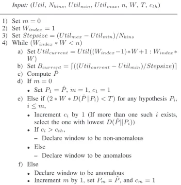
AlgorithmANOMALYDETECTION USINGMULTINOMIAL GOODNESS-OF-FIT Input:(𝑈𝑡𝑖𝑙,𝑁𝑏𝑖𝑛𝑠,𝑈𝑡𝑖𝑙𝑚𝑖𝑛,𝑈𝑡𝑖𝑙𝑚𝑎𝑥,𝑛,𝑊,𝑇,𝑐𝑡ℎ) 1) Set𝑚= 0 2) Set𝑊_{𝑖𝑛𝑑𝑒𝑥}= 1 3) Set𝑆𝑡𝑒𝑝𝑠𝑖𝑧𝑒= (𝑈𝑡𝑖𝑙_𝑚𝑎𝑥−𝑈𝑡𝑖𝑙_𝑚𝑖𝑛)/𝑁_{𝑏𝑖𝑛𝑠} 4) While(𝑊_{𝑖𝑛𝑑𝑒𝑥}∗𝑊 < 𝑛) a) Set𝑈𝑡𝑖𝑙_{𝑐𝑢𝑟𝑟𝑒𝑛𝑡}=𝑈𝑡𝑖𝑙((𝑊_{𝑖𝑛𝑑𝑒𝑥}−1)∗𝑊+1 :𝑊_{𝑖𝑛𝑑𝑒𝑥}∗ 𝑊) b) Set𝐵_{𝑐𝑢𝑟𝑟𝑒𝑛𝑡}=⌈((𝑈𝑡𝑖𝑙_{𝑐𝑢𝑟𝑟𝑒𝑛𝑡}−𝑈𝑡𝑖𝑙_𝑚𝑖𝑛)/𝑆𝑡𝑒𝑝𝑠𝑖𝑧𝑒)⌉ c) Compute𝑃ˆ d) If𝑚= 0 ∙ Set𝑃₁= ˆ𝑃,𝑚= 1,𝑐₁= 1

e) Else if(2∗𝑊∗𝐷( ˆ𝑃∣∣𝑃_𝑖)< 𝑇)for any hypothesis𝑃_𝑖,

𝑖≤𝑚,

∙ Increment𝑐_𝑖 by 1 (If more than one such 𝑖 exists, select the one with lowest𝐷( ˆ𝑃∣∣𝑃𝑖))

∙ If𝑐𝑖> 𝑐𝑡ℎ,

– Declare window to be non-anomalous

∙ Else

– Declare window to be anomalous f) Else

∙ Declare window to be anomalous

∙ Increment𝑚by1, set𝑃_𝑚 =𝑃ˆ, and𝑐_𝑚= 1

Fig. 1. Algorithm for anomaly detection with multiple null hypotheses

The algorithms works as follows. The current window is selected in Step 4a) and the values in the window are quantized in Step 4b). The algorithm computes the empirical frequency 𝑃ˆ of the current window as in Step 4c). Observe that 𝑃₁, 𝑃₂, . . . , 𝑃_𝑚 denote the 𝑚 null hypotheses at any point in time. A test-statistic involving 𝑃ˆ and each of the

𝑃𝑖s is computed and compared to the threshold 𝑇 in Step

4e). If the test-statistic exceeds the threshold for all of the null-hypotheses, the window is declared anomalous, 𝑚 is incremented by 1 and a new hypothesis is created based on the current window. If the smallest test-statistic is less than the threshold but corresponds to a hypothesis that was accepted less than 𝑐_𝑡ℎ times in the past, then the window is declared anomalous, but the number of appearances of that hypothesis is incremented. If neither of the two conditions is satisfied, the window is declared non-anomalous and the appropriate book-keeping performed.

The relative entropy based approaches described here have several advantages. They are non-parametric, namely they do not assume a particular form for the distribution of the data. They can be easily extended to handle multi-dimensional time-series thereby incorporating correlation, and can be adapted to workloads whose distribution changes over time. While relative entropy and hypothesis testing approaches have been used for anomaly detection, we are not aware of any work that uses it in the context of multinomial goodness of fit test. The latter provides a systematic way (based on the cdf of the chi-squared distribution) to choose a threshold above which alarms are raised. This feature is not always present in other works using the relative entropy metric. We also extend the technique in a novel manner to adapt to multiple operating states and for detecting contextual anomalies.

All the algorithms that we propose are computationally lightweight. The algorithms require computing statistics for current window and updating historical statistics. The compu-tation overhead for the current window statistics is negligible. Updating quantities such as mean and standard deviation can clearly be performed in linear time, Further this can be done in an online manner with very little memory as only the sum of the observed values and the sum of the squares of the observed values need to be maintained. For the Tukey method, we need to compute quantiles, and for the relative entropy method, the empirical frequency of previous windows. These can also be computed in time linear in the input. Further, these quantities can be well-approximated in one pass with limited memory, without having to store all the observed data points [22].

IV. THERESULTS

We tested the algorithms discussed in Section III on two different types of data. The first data set was one where we could inject anomalies and validate the results returned by our algorithms. It was obtained from an experimental setup with a representative internet service - RUBiS [17], a distributed online service implementing the core functionality of an auction site. The second type of data set was collected from production data centers.

Method Statistics Over Recall FPR Gaussian (windowed) Entire past 0.06 0.02 Gaussian (windowed) Recent windows 0.06 0.02 Gaussian(smoothed) Entire Past 0.58 0.08 Tukey(smoothed) Entire Past 0.76 0.04 Relative entropy Entire past 0.46 0.04 Relative entropy Recent past 0.74 0.04 Relative entropy Multiple Hypotheses 0.86 0.04

TABLE I

RECALL AND FALSE POSITIVE RATES FOR DIFFERENT TECHNIQUES WITH RUBISDATA

A. RUBiS Testbed Results

The RUBiS testbed uses 5 virtual machines (VM1 to VM5) on Xen platform hosted on two physical servers (Host1 and Host2). VM1, VM2, and VM3 are created on Host1. The frontend server processing or redirecting service requests runs in VM1. The application server handling the application logic runs in VM2. The database backend server is deployed on VM3. The deployment is typical in its use of multiple VMs and the consolidation of them onto a smaller number of hosts. A request load generator and an anomaly injector are running on two virtual machines, VM4 and VM5, on Host2. The generator creates 10 hours worth of service request load for Host1 where the auction site resides. The load emulates concurrent clients, sessions, and human activities. During the experiment, the anomaly injector injects 50 anomalies into the RUBiS online service in Host1. Those 50 anomalies come from major sources of failures or performance issues in online services [18]. We inject them into the testbed using a uniform distribution. The virtual machine and host metrics are collected/analyzed in an anomaly detector.

We present the results of analyzing the CPU utilizations in Table I. The CPU utilization data was quantized into 33 equally spaced bins, and for the windowing techniques, the window length was set to100. For algorithms that use only the recent past,10windows of data were used. For the Gaussian methods, for each window, anomaly detection was performed on the CPU utilization of each of the three virtual servers and an alarm raised if an anomaly is detected in at least one of them. For the relative entropy methods, the sum of the test statistics of each of the servers is compared to a threshold (computed based on the fact that the sum of chi-squared random variables is a chi-chi-squared random variable). As mentioned, there were total 50anomalies injected, and in our evaluation, an anomaly is said to be detected if an alarm is raised in a window containing the anomaly. The results are presented in terms of statistical metrics - Recall and False Positive Rate (FPR).

𝑅𝑒𝑐𝑎𝑙𝑙= # of succesful detections

# of total anomalies (2)

False Positive Rate (FPR)=# of false alarms

# of total alarms. (3)

From Table I, it is clear that the windowed Gaussian tech-niques perform poorly when applied to the RUBiS data.

The relative entropy-based algorithms and the Tukey method perform much better with the multiple hypothesis relative entropy technique giving the best results (detecting 86% of the anomalies with a minimal false positive rate). Also, using the few past windows to select the null hypothesis provides better accuracy than using the entire past.

B. Production Data Center Results

In this section, we report results from analyzing data col-lected from two different real world customer production data centers over a 30and60 day period respectively (henceforth called CUST1 and CUST2 respectively) [19]. The metrics such as CPU and Memory utilization are sampled every 5 minutes. We segmented this data by hour of day, and day of week for both CUST1 and CUST2, and applied the anomaly detection methods over them, thus performing context-based evaluations. We primarily report results in this section on these context-based evaluations only. Also, since this is data from production data centers, we had no control of the anomalies that manifested, nor do we have knowledge about them. So, in our evaluations, we simply report the number of anomalies detected by the various techniques, and do a comparison among them. The implementation for the Gaussian techniques is based on the industry-standard MASF approach [1].

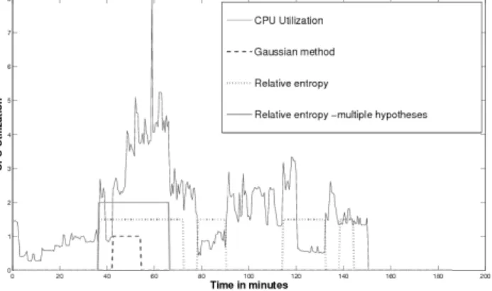
In Figure 2, we present a representative plot of the win-dowed techniques on the data of one of the servers for CUST1 contextualizing the data based on hour of day, as explained in Section III. The results shown are for a fixed hour during the day and for CPU Utilization data (this data is measured in terms of number of cores utilized ranging from 0 to 8). The alarms raised by different techniques are shown. To interpret the plots, note that if any of the curves is non-zero, then it implies that an alarm was raised by the technique corresponding to the curve. The heights of the curves do not carry any further meaning. We observe that the Gaussian threshold based method does not detect the first unusual increase in CPU utilization as soon as the Goodness-of-fit based methods. The multiple hypothesis version learns the behavior of the system and does not raise an alarm during similar subsequent increases.

Fig. 2. Anomaly detection on real-world data (CUST1)

exam-Hour of day # Anomalies # Anomalies # Anomalies Common Unique to RE Unique to Unique to

(Relative (Gaussian) (Tukey) Anomalies Gaussian Tukey

Entropy-RE) 0000 6 7 7 6 0 0 0 0100 4 6 1 1 0 2 0 0200 2 4 0 0 0 2 0 0300 5 4 2 1 2 0 0 0400 5 5 2 2 0 0 0 0500 4 5 2 1 1 1 0 0600 5 7 3 3 0 2 0 0700 4 6 7 4 0 0 1 0800 6 2 3 2 3 0 0 0900 7 2 14 2 0 0 7 1000 6 2 13 2 0 0 7 1100 7 2 3 1 5 0 0 1200 4 2 2 2 2 0 0 1300 1 2 1 1 0 1 0 1400 5 5 5 4 1 0 0 1500 6 5 12 4 1 0 6 1600 4 5 2 2 1 2 0 1700 4 3 3 2 2 0 0 1800 4 3 0 0 1 0 0 1900 5 3 3 3 2 0 0 2000 3 2 0 0 2 1 0 2100 6 5 8 4 1 0 2 2200 5 4 0 0 2 1 0 2300 6 10 6 5 0 3 0 TABLE II

COMPARISON OF VARIOUS TECHNIQUES ON REAL CUSTOMER DATA(CUST2): NUMBER OF ANOMALIES DETECTED BY EACH TECHNIQUE IN EACH HOUR FOR WEEKDAYS

ined the CPU utilization of one of the servers and interleaved the data according to hour of day. More specifically, for each

𝑥 ∈ {0,1,2, . . . ,23}, we grouped together all the measure-ments made between𝑥hours and𝑥+1hours on weekdays. We tested the pointwise Gaussian and Tukey techniques, as well as the relative entropy technique with multiple hypotheses. To determine the limits for the pointwise Gaussian and Tukey techniques, we used the first half of the data set to estimate the mean, standard deviation and relevant quantiles. We then applied the thresholds on the second half of the data set to detect anomalies. The server in question had been allocated a maximum of 16 cores and thus the values of CPU utilization ranged between 0.0 and 16.0. To apply the relative entropy detector, we used a bin width of 2.0 which corresponds to 8 bins. The window size was 12data points which corresponds to an hour. Thus the relative entropy detector, at the end of each hour, declares that window to be anomalous or otherwise. To facilitate an apples-for-apples comparison, we processed the alarms raised by the Gaussian and Tukey methods as follows. For each of the techniques, if within one window at least one alarm is raised, then the window is deemed anomalous. This way we are able to compare the number of windows that each of the techniques flags as anomalous. The above comparison is performed for each of the24hours. The results are presented in Table II.

The first column in Table II specifies the hour of day that was analyzed. The next three columns indicate number of anomalies detected by the three techniques. The fifth column states the number of anomalies detected by all of them and the sixth, seventh and eighth columns the anomalies that were uniquely detected by each of the techniques. For instance the sixth column records the number of anomalies detected by the

relative entropy technique but not by the other two.

To briefly summarize the results, we observe that in most cases the relative entropy technique identifies the anomalies detected by the other two techniques, and flags a few more as well. There are three notable exceptions hours - 0900, 1000 and1500where the Tukey method flags6−7more anomalies than the other techniques. A closer examination of the data corresponding to these hours reveals that the CPU utilization during these hours was mostly very low (<0.5) leading to the inter-quartile range being very small and therefore resulting in a very low upper threshold. As a result, the algorithm flagged a large number of windows as anomalous and it is reasonable to surmise that some of these may be false alarms. On the other hand, the data corresponding to hour 1100 results in the relative entropy technique returning 5 anomalies that the other two techniques do not flag. Some of these anomalies are interesting when examined closely. The typical behavior of the CPU utilization is as follows: it hovers between 0.0 and 2.0 with occasional spikes. But often after spiking to a value greater than6.0 for a few measurements, it drops back down to a value around2.0. But in a couple of cases, the value does not drop down entirely and remains between4.0and6.0, indicating perhaps a stuck thread. The Gaussian and Tukey methods do not catch this anomaly as it does not manifest as an extreme value. However, it is interesting that the relative entropy is able to catch this.

Finally, we present results for data segmented by hour for a given day of the week only. In other words, we string together data by each hour for a given day over the entire data collection period. The results we present consist of analyzing the hours between 10 AM and 5 PM on Mondays only over the collection period. Both cpu-utilization and memory utilization

Hour Parameter # Anomalies # Anomalies # Common

of day (Gaussian) (Tukey) Anomalies

10 CPU 0 0 0 10 Memory 12 0 0 11 CPU 0 26 0 11 Memory 0 0 0 12 CPU 3 11 3 12 Memory 0 0 0 13 CPU 2 2 2 13 Memory 1 1 1 14 CPU 1 0 0 14 Memory 0 0 0 15 CPU 15 11 11 15 Memory 12 0 0 16 CPU 0 0 0 16 Memory 0 0 0 17 CPU 0 0 0 17 Memory 0 0 0 TABLE III

COMPARISON OFGAUSSIAN ANDTUKEY METHODS FORMONDAYS ONLY (CUST2). THE DATA IS ANALYZED BY HOUR OF DAY AND DAY OF WEEK.

methods were analyzed. The summary of the analysis is that while fewer anomalies are flagged there are some significant blips. This is presumably due to the server utilization over short, hourly periods tend to be stable with sudden bursts of activity. The data is summarized in Table III. It is clear from the tabulated results that CPU-utilization shows more variability than Memory utilization. The two anomaly detec-tion techniques flag few anomalies common to each other. Only in the hours of 12, 13, and 15 do they trigger common anomalies albeit few. Note that there is significant variability in the performance of the two techniques. In the 10 A.M. hour, while the Gaussian technique flags 12 anomalies, the Tukey trigger none for memory utilization. On the other hand, in the hour 11 A.M. hour, the Gaussian technique does not flag any anomalies, while the Tukey flags as many as 13 each of lower and upper anomalies in cpu-utilization (total 26). Although, the Tukey method flags more anomalies overall (51) as opposed to 46 by the Gaussian technique, the Tukey is better suited to anomaly detection because of its generality, flexibility, and ease of computation.

V. DISCUSSION

As seen, the statistical algorithms for anomaly detection analyze monitoring data over historical periods to make their decisions. This historical period could be the entire past of the workload operation, or it could be restricted to recent past values only. In either of these cases, the considered data could be organized based on continuous history over time, or it could be segregated by context, e.g. hour of day or day or week. Which historical period and organization type is chosen has an effect on the results of the anomaly detection algorithms. For example, for Gaussian and Tukey methods, this will affect the value of thresholds chosen, and for Relative Entropy, it will affect the null hypotheses against which the current window is evaluated.

Several factors play a role in selecting the appropriate historical period. Workload behavior and pattern is one of them. If the workload has a periodic behavior, then recent past values that can give enough statistical significance might

suffice. Further, if the pattern is based on weekly or hourly behavior, then organizing the data by context is preferable. If the workload is long running and has exhibited aperiodic behavior in the past, the entire past data would help smooth out averages. If the workload has varying behavior that is time-dependent or if it is originating from virtual machines that have been migrated or subject to varying resource allocation in shared environments, considering only recent windows might help to eliminate noise from past variable behavior.

In enterprise environments with dedicated infrastructures, it might be straightforward to select the appropriate historical period and organization of data. However, in cloud and utility computing environments with limited prior knowledge of workload behavior, high churn, and shared infrastructure for workloads, the most appropriate historical period and organi-zation of data to choose may be challenging and expensive to determine over large scale. Instead, we suggest an alternative approach in which at any given time, we do multiple runs of the anomaly detection algorithm in parallel, each run leveraging data analyzed from a different historical period. The results from these individual runs could then be combined to provide overall insight and asystem statusindicator to the administrator. For performing of multiple runs to be feasible, the algorithm has to be lightweight. As discussed in previous sections, our proposed algorithms are lightweight and could be used for this approach.

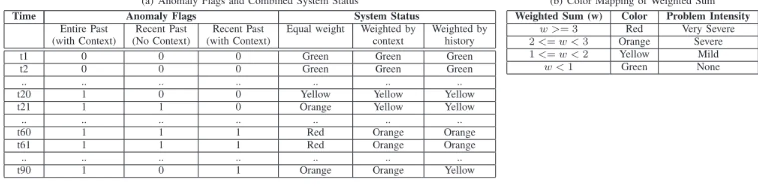
Table IV(a) illustrates how the approach would work. The table shows a sample trace and output of an anomaly detection algorithm over time using data from different historical periods (entire past, recent past) with and without consideration of context. An output of 1 indicates that an anomaly flag is raised for that time period, and 0 indicates otherwise. To combine the results, we propose a weighted combination of these output flags. This weighted combination can be mapped to a coloring scheme shown in Table IV(b). The color represents the overall system status for the system being monitored. Table IV(a) shows the results when different weights are used. Column 5 shows the system status with equal weights to the different historical periods, Column 6 shows the system status when workload patterns (hence context) are given higher weight (1, 0.5, 1 for Columns 2, 3 and 4 respectively), and Column 7 shows the system status when historical knowledge is given higher weight (1, 0.5, 0.5 for Columns 2, 3, 4).

While not shown, it is easy to see that the same approach can be extended to combine results from multiple algorithms as well. This could lead to two level of combinations - com-binations for different historical periods for a given algorithm, and then combinations of those across multiple algorithms. The feasibility of this hybrid approach would however be dependent on the complexity of algorithms so as to be able to execute multiple algorithms on online data.

More broadly, the discussion in this section points us to the different dimensions that anomaly detection algorithms have to consider, and how a systematic approach can enable us to obtain improved understanding of system behavior in complex, and large-scale shared computing infrastructures such as being

(a) Anomaly Flags and Combined System Status

Time Anomaly Flags System Status

Entire Past Recent Past Recent Past Equal weight Weighted by Weighted by (with Context) (No Context) (with Context) context history

t1 0 0 0 Green Green Green

t2 0 0 0 Green Green Green

.. .. .. .. .. .. ..

t20 1 0 0 Yellow Yellow Yellow

t21 1 1 0 Orange Yellow Yellow

.. .. .. .. .. .. ..

t60 1 1 1 Red Orange Orange

t61 1 1 1 Red Orange Orange

.. .. .. .. .. .. ..

t90 1 0 1 Orange Orange Yellow

(b) Color Mapping of Weighted Sum

Weighted Sum (w) Color Problem Intensity

𝑤 >= 3 Red Very Severe

2<=𝑤 <3 Orange Severe

1<=𝑤 <2 Yellow Mild

𝑤 <1 Green None

TABLE IV

ILLUSTRATION OFCOMBINEDSYSTEMSTATUS

represented by utility clouds.

VI. RELATEDWORK

Most of current industry monitoring tools use fixed thresh-olds for anomaly detection. Fixed upper and lower bounds are determined apriori and remain constant during the entire process of anomaly detection. MASF [1] is one of the popular threshold-based techniques being adopted in industry. MASF applies thresholds to data segmented by hour of day, and day of week. As discussed earlier, these techniques have limitations of accuracy and false alarm rates due to their assumed data distributions, and limited adaptibility to changing workloads. They have poor scalability and lack of correlation analysis.

Prior academic work has developed many useful methods for anomaly detection, typically based on statistical tech-niques [2], [3], [4], [5], [6], [7], [8]. A summary is provided by [21]. However, few of them can operate at the scale of future data center or cloud computing systems and/or have the ’lightweight’ characteristic desired for online operation. Reasons include their use of statistical algorithms with high computing overheads and their use of onerously large amounts of raw metric information. In addition, they may require prior knowledge about application SLOs, service implementations, request semantics, or they are focused on solving certain well-defined problems at specific levels of abstraction (i.e., metric levels) in data center systems.

In contrast, the techniques we propose are lightweight techniques that systematically improve on the state of art techniques widely adopted in industry. We have proposed tech-niques to improve on current point fixed-threshold approaches, and we have also developed new windowing-based approaches that observe changes in the distribution of data. Our techniques are adaptable and can learn the workload characteristics over time, improving accuracy and reducing false alarms. They also meet the scalability needs of future data centers, are applicable to multiple contexts of data (catching contextual anomalies), and can be applied to multiple metrics in data centers.

VII. CONCLUSIONS ANDFUTUREWORK

Anomaly Detection is an important component for closed loop management in data centers. In this paper, we pre-sented statistical approaches for online detection of anomalies.

Specifically, we have presented methods based on Tukey and Relative Entropy statistics, and experimentally evaluated them. The proposed approaches are lightweight and improve upon prevalent Gaussian-based approaches.

As ongoing work, we are performing more evaluations on synthetic as well as customer data. We are also exploring further refinements to the techniques presented in this paper for multiple metrics and for aggregation across multiple machines at large scale. We also plan to do evaluations with other cloud workloads and benchmarks.

REFERENCES

[1] Jeffrey P. Buzen and et. al., MASF: Multivariate Adaptive Statistical Filtering, CMG Confernce, 1995.

[2] S. Agarwala andet. al., E2EProf: Automated End-to-End Performance Management for Enterprise Systems, DSN, 2007.

[3] S. Agarwala and K. Schwan, SysProf: Online Distributed Behavior Diagnosis through Fine-grain System Monitoring, ICDCS, 2006. [4] Ira Cohen andet. al., Correlating Instrumentation Data to System States:

A Building Block for Automated Diagnosis and Control, OSDI, 2004. [5] Bahl, Paramvir andet. al., Towards highly reliable enterprise network

services via inference of multi-level dependencies, SIGCOMM, 2007. [6] Chen, Mike Y. and et. al., Pinpoint: Problem Determination in Large,

Dynamic Internet Services, DSN, 2002.

[7] A. Barham, andet. al., Using magpie for request extraction and workload modelling, OSDI’04, 2004.

[8] M.K. Aguilera andet. al., Performance debugging for distributed systems of black boxes, SOSP ’03, 2003.

[9] J. Tukey, Exploratory Data Analysis, Addison Wesley, MA, 1977. [10] D. Montgomery andet. al., Engineering Statistics, Wiley, 2006. [11] I. Daubechies, Ten Lectures on Wavelets, Applied Mathematics, 1992. [12] R. Baeza-Yates andet. al., Modern Information retrieval,1999 [13] R. Johnson andet. al., Applied Multivariate Statistical Analysis, 2001 [14] S. Mallat, A Theory of Multiresolution Signal Decomposition: The

Wavelet Representation, Academic Press, 2009.

[15] T. M. Cover andet. al., Elements of Information Theory, 1991. [16] E. L. Lehmann andet, al., Testing Statistical Hypothesis, Springer, 2005. [17] E. Cecchet, andet. al., Performance and scalability of ejb applications,

OOPSLA, 2002.

[18] C. Wang andet. al., Online detection of utility cloud anomalies using metric distributions, NOMS, 2010.

[19] Anonymized Production Data Center Logs, HP Internal Correspondence. [20] C. Bishop, Neural networks for pattern recognition

[21] V.Chandola, andet. al., Anomaly Detection : A Survey, ACM Comput-ing Surveys, 2009

[22] G. Cormode, andet. al.,An improved data stream summary: The count-min sketch and its applications, Journal of Algorithms, 2005.