Copyright © UNU-WIDER 2008
1 Bank of Thailand, Thailand, e-mail: ManopU@bot.or.th; 2 University of Nottingham, UK, e-mail: Oliver.Morrissey@nottingham.ac.uk; 3 Kiel Institute of World Economics and Christian-Albrechts University, Germany, e-mail: holger.goerg@ifw-kiel.de
This study has been prepared within the UNU-WIDER project on Southern Engines of Global Growth, co-directed by Amelia U. Santos-Paulino and Guanghua Wan.
UNU-WIDER gratefully acknowledges the financial contributions to the research programme by the governments of Denmark (Royal Ministry of Foreign Affairs), Finland (Ministry for Foreign Affairs), Norway (Royal Ministry of Foreign Affairs), Sweden (Swedish International Development Cooperation Agency—Sida) and the United Kingdom (Department for International Development).
ISSN 1810-2611 ISBN 978-92-9230-158-3
Research Paper No. 2008/102
Exchange Rates and Outward
Foreign Direct Investment
US FDI in Emerging Economies
Manop Udomkerdmongkol,
1Oliver Morrissey,
2and Holger Görg
3 November 2008Abstract
The paper investigates the impact of exchange rates on US foreign direct investment (FDI) flows to a sample of 16 emerging market countries using annual panel data for the period 1990-2002. Three separate exchange rate effects are considered: the value of the local currency (a cheaper currency attracts FDI); expected changes in the exchange rate (expected devaluation implies FDI is postponed); and exchange rate volatility (discourages FDI). The results reveal a negative relationship between FDI and more expensive local currency, the expectation of local currency depreciation, and volatile exchange rates. Stable exchange rate management can be important in attracting FDI. Keywords: exchange rate, FDI, foreign exchange
The World Institute for Development Economics Research (WIDER) was established by the United Nations University (UNU) as its first research and training centre and started work in Helsinki, Finland in 1985. The Institute undertakes applied research and policy analysis on structural changes affecting the developing and transitional economies, provides a forum for the advocacy of policies leading to robust, equitable and environmentally sustainable growth, and promotes capacity strengthening and training in the field of economic and social policy making. Work is carried out by staff researchers and visiting scholars in Helsinki and through networks of collaborating scholars and institutions around the world.
www.wider.unu.edu publications@wider.unu.edu
UNU World Institute for Development Economics Research (UNU-WIDER) Katajanokanlaituri 6 B, 00160 Helsinki, Finland
Typescript prepared by Janis Vehmaan-Kreula at UNU-WIDER
The views expressed in this publication are those of the author(s). Publication does not imply endorsement by the Institute or the United Nations University, nor by the programme/project sponsors, of any of the views expressed.
Acknowledgements
The views expressed in this paper are those of the authors and do not necessarily represent those of the Bank of Thailand or Bank of Thailand policy. Helpful comments were received from Diego Moccero.
1 Introduction
Empirical studies on foreign direct investment (FDI) and exchange rate linkages are important for the formulation of FDI policies given that there has been an increase in the number of countries adopting floating exchange rates (or abandoning fixed pegs, if only temporarily), so research on the ways in which exchange rates can influence incentives for foreign investment is timely. Although many studies have examined whether exchange rates are determinants of FDI inflows to host countries, they mostly focus on the level of the exchange rate (as a current price effect). The existing literature has generally found a positive effect of local currency depreciation on inward FDI. Various reasons are suggested, with some studies clarifying the effect of the exchange rates as a supply-side or push factor on the FDI inflows. Specifically, a stronger home currency increases outward FDI (see Froot and Stein 1991; Klein and Rosengren 1994). Others explain it as the allocation effect – FDI goes to countries where the currency is weaker as a given amount of foreign currency can buy more investment (see Cushman 1985, 1988; Campa 1993; Goldberg and Kolstad 1995; Blonigen 1997; Chakrabarti and Scholnick 2002).
Most existing studies on the effect of exchange rates consider FDI into developed countries. Froot and Stein (1991) find that the US dollarvalue is statistically negatively correlated with FDI (in US dollar terms) from industrialized countries to the US over 1974-87. Blonigen (1997) finds that depreciation of the US dollar is significantly related to the number of Japanese acquisitions in the US. Chakrabarti and Scholnick (2002) find no consistent effect of US dollar exchange rates on US FDI to 20 OECD countries over 1982-95. Few studies have examined the role of exchange rates on FDI to developing countries.
This paper contributes to the literature on the impact of exchange rates on FDI by concentrating on US FDI to 16 emerging market economies over 1990-2002. Three distinct exchange rate effects are considered. First, the average official bilateral exchange rate (local currency units against US dollar) adjusted for inflation is used to capture the ‘cost of investment’ effect. Second, changes in real effective exchange rate indices (REER) are used to capture the effect of expectations for changes in the value of the local currency on inward FDI. Third, an estimate of the temporary component of the bilateral exchange rate is used to capture the effect of host countries’ exchange rate volatility, which is expected to discourage FDI inflows (Campa 1993). This paper therefore specifically tests three hypotheses:
1. FDI rises when devaluation occurs, that is, devaluation lowers the cost of investment to foreigners and so increases FDI (from the country whose currency has become more valuable).
2. Expected future devaluation of the local currency lowers current inward FDI. If foreign investors expect that a currency will be devalued, they will postpone their investment until devaluation occurs.
3. Exchange rate volatility discourages FDI, that is, foreign investors prefer countries in which the foreign ‘exchange value’ of their investment is more stable.
The results of the analysis provide evidence in support of all three hypotheses. Moreover, we find that good economic conditions and foreign investors’ confidence in political and economic conditions of the countries are significant determinants of inward FDI. As a result, a government’s ability to provide a stable investment environment for foreign entrepreneurs will secure greater amounts of FDI inflows to its country.
Section 2 outlines the theoretical background. The subsequent section describes the data set and the econometric framework, followed by a discussion of the results. Finally, the last section summarizes findings and discusses implications of policy in attracting FDI.
2 Theoretical framework
The analysis is motivated by the model of Chakrabarti and Scholnick (2002), to suggest specification and variables, who argue that owing to inelasticity in expectations, investors do not revise their expectations of future exchange rates to the full extent of changes in the current exchange rate. Thus, if they believe that a devaluation of a foreign currency will be followed by a mean reversion of the exchange rate, this implies that immediately after devaluation the foreign currency would be temporarily ‘cheap’ (temporary change in foreign currency value). As a consequence, ceteris paribus, FDI would flow to the country under these circumstances because foreign assets currently appear to be cheap relative to their expected future income stream.
Assume that a multinational enterprise (MNE) is contemplating FDI in a host country. The project concerned is subject to diminishing returns to scale. Also, for simplicity, assume that the MNE makes a single payment at a certain point in the future.1 The expected net payoff to the MNE from the venture is expressed as:
( ) ( )
( )
0 1 1 r C N e e E N R N⎢⎣⎡ ⎥⎦⎤− + = π (1)where N is a measure of the scale of the project, R is revenue in local currency occurring at a future point in time for unit N, C is the cost of the project in host country currency payable up-front for unit N, e0 is the exchange rate (home country currency unit per host country currency unit) at the time of the investment, E(e1) is the expected exchange rate when the project pays back, and r is the opportunity cost of capital over the project’s life.
Given diminishing returns to scale, the MNE maximizes expected net payoff value by choosing an appropriate value of N. There exists an expected dollar-profit maximizing value of N which solves the problem. The optimal level of N, say N*, is a function of the opportunity cost of capital and the expected depreciation d = log[e0] – log[E(e1)] of the home country currency, such that:
1 The authors support this assumption with an argument that although most FDI projects would lead to a stream of earnings rather than a single earning, such a stream may be represented by a single payment coming at the end of project.
N* = N*(r,d) ; ∂N*/∂r < 0and∂N*/∂d < 0 (2)
Given the notion of inelasticity in expectation (Frankel and Froot 1987), agents do not revise their expectations of the future exchange rate to the full extent of changes in current exchange rate. Analytically,
dE(e1) / de0 < 1 (3) From equations (2) and (3),
dN* / de0< 0 (4) In other words, an appreciation in a local currency raises the expectation of the future level of the exchange rate by less than the amount of current appreciation, creating expectation of a future devaluation (of the currency), and reducing FDI inflows to the host country. The opposite happens in the case of depreciation (Chakrabarti and Scholnick 2002).
The effect can be seen most easily using a stylized example. Imagine first that a US investor is interested in buying a plant in, say, Thailand. The plant costs 50 million baht (Thai currency unit). The investor has one million US dollars available and no other sources of finance. If the exchange rate is 25 baht/US dollar the investor cannot purchase the plant. If the dollar appreciates to a value of 50 baht the investor is able to make the investment. Thus, the depreciation of the baht has increased the relative wealth of investors and encouraged foreign investment. Moreover, the investor may expect the dollar would soon depreciate to a value of, say, 40 baht. The investor would gain benefits from the expected devaluation when repatriating profits (in dollar terms). In conclusion, the devaluation of the local currency and the expectation of (future) local currency appreciation lead to higher FDI inflows to the country.
The effects of exchange rates will depend on the motives for FDI. For example, the model is less evidently appropriate for explaining export-oriented FDI. In this case, although the cost effect persists (current devaluation implies investment costs less to the foreign investor), foreign investors anticipating an appreciation of the local currency might postpone export-oriented FDI (the reverse of the above). This arises if exports are invoiced in the local currency: future appreciation implies that the expected price of exports rises (more foreign currency required to buy a unit of local currency) so demand falls.2 As a result, FDI would not be higher in the country if there is an expectation of local currency appreciation. This possibility cannot be incorporated due to unavailability of detailed data on the purpose of FDI; in practice, much will depend on the internal invoicing practices of the MNE, so any effect is muted.
2 If exports are priced in the foreign currency the (world) price is unchanged so there is no demand-side effect. However, the local affiliate receives less domestic currency per unit of exports, so there may be an adverse supply-side effect that discourages investment.
3 Empirical method and data
The sample (determined by data availability) covers 16 emerging market economies over 1990-2002, using annual data from the International Monetary Fund (IMF 2003).3 The countries consist of 8 in Latin America (Bolivia, Chile, Colombia, Costa Rica, Dominican Republic, Paraguay, Uruguay, and Venezuela), 5 countries from Asia (China, Malaysia, Pakistan, the Philippines, and Thailand), and 3 African countries (Morocco, South Africa, and Tunisia). Details on the data are provided in Appendix A. As the aim is to test three hypotheses – FDI rises when devaluation occurs; an expected devaluation of the currency increases current inward FDI; and exchange rate volatility discourages FDI – a primary concern is devising separate measures or indicators for each exchange rate effect. The average official bilateral exchange rates (local currency unit against US dollar) adjusted for inflation is a standard measure for the exchange rate level that may influence the allocation of FDI (Cushman 1985, 1988; Froot and Stein 1991; Klein and Rosengren 1994; Goldberg and Kolstad 1995; Blonigen 1997; Goldberg and Klein 1998). As elaborated below, we use a measure of the real effective exchange rate to capture expectations and a measure of cyclical and irregular components of the exchange rate as a proxy for volatility.4
The change in (the log of) a host country’s real effective exchange rate (REER)5 is used as a proxy for expectations of what is likely to happen to the value of the local currency. Ideally, we would consider if the REER is above or below its equilibrium value. As we do not have data on this, we assume that it tends on average to revert to the equilibrium (or, more strictly, that foreign investors interpret trends in the REER as movement away from equilibrium), so the change ‘predicts’ how nominal exchange rate will move in future to restore equilibrium. An increase (decrease) in REER implies that MNEs may expect local currency devaluation (appreciation), assuming that first difference proxies deviation from equilibrium. Goldfajn and Valdés (1999) empirically analyse a broad range of real exchange rate appreciation cases in 93 countries over the period 1960-94 and argue that real appreciations or overvaluations are reversed with nominal depreciations.6 In general, an overvalued currency generates unsustainable current account deficits through the loss of competitiveness leading to a possible recession and
3 High frequency (monthly or daily) data on exchange rates are not available for many countries (for example, Tunisia; Morocco; Pakistan; China; Malaysia; Bolivia; Costa Rica; Paraguay; Uruguay; Venezuela).
4 Chakrabarti and Scholnick (2002) measure exchange rate volatility by standard deviation and exchange rate shock as skewness of the exchange rate, both derived from high frequency data. We only have annual data. Furthermore, due to data limitations, exchange rate data from futures markets cannot be used to capture exchange rate expectations.
5 The IMF defines REER as nominal effective exchange rate adjusted for relative movements in national price indicators of a home country and selected countries.
6 Goldfajn and Valdés (1999) calculate the overvaluation series as deviations of the real exchange rate from a Hodrick-Prescott (H-P) filter series. Chinn (2005) argues that calculating the overvaluation as a deviation from an estimated trend is not a valid procedure unless the time series being examined are
I(0) variables. In fact, exchange rate series of emerging markets do not appear to be I(0) processes;
hence, the H-P filter procedure is not justified. Nonetheless, REER can be used to assess the competitiveness and overvaluation in a host country.
loss of reserves. Policy makers thus correct the overvaluation through nominal devaluation.
Perhaps the most common and natural application of REER is to assess a country’s competitiveness, albeit imperfectly, relative to its main trading partners. This method refers to a calculation of average exchange rates of major trading partners by giving weights in accordance with each country’s trade proportion prior to adjusting it to differences in inflation rates between a country and its trade partners. REER can play an important and useful role in conveying key summary information to policy makers, for example on (changing) competitiveness and overvaluation. To decide whether the REER at a given time is too weak or strong, that is, has moved away from equilibrium, the measure used in the analysis is annual changes (ΔREER = REERt – REERt-1, measured in logs).
If the domestic economy is improving relative to its trading partners, attracting both FDI and portfolio investment, the real exchange rate should be appreciating (or the local currency is over-valued) so the REER is increasing. The overvalued currency generates a higher than anticipated current account deficit and reduces competitiveness, which leads to weaker economic performance and loss of reserves. The central bank therefore corrects the overvaluation through nominal devaluation (Goldfajn and Valdés 1999). Thus, an increasing REER (real exchange rate appreciation) implies that the local currency would devalue in the near future; current inflows of FDI would decrease as foreign investors await the anticipated cheaper currency (Chakrabarti and Scholnick 2002). The opposite happens in the case of real exchange rate depreciation.
While there are various ways of measuring exchange rate volatility, the principal concern here is to identify the (extent of) cyclical and irregular components of exchange rate movements.7 An exchange rate can be considered as the sum of three components:
exchange rate = trend component + cyclical component + irregular component
Newbold (1995) shows that cyclical and irregular elements appear to exhibit oscillatory and unpredictable behaviour in time series (exchange rates series in particular). In other words, the two elements in the temporary component generate exchange rate variability and can therefore be used as a measure of exchange rate volatility. We utilise the H-P filter approach (Hodrick and Prescott 1997) to estimate the trend component. The trend can then be deducted to leave the volatile components:
exchange rate – trend component = cyclical component + irregular component
The econometric model to be estimated is:
FDIi,t = β0 + β1ΔREERi,t + β2FXDi,t + β3TFXDi,t+ β4Xi,t+ µi + εi,t (5) where FDIi,t is US FDI inflows to country i, ΔREERi,t is change in log of real effective
exchange rate index (REER), FXDi,t is bilateral exchange rates adjusted for inflation (in
logs), TFXDi,t is the temporary (cyclical and irregular) component of bilateral exchange
rates (logs), Xi,t is a vector capturing other country level determinants of inward FDI,
7 One may argue that seasonal factor may cause exchange rate volatility but as we use annual data this can be dropped from consideration.
t i,
ε is the white noise error term and µi is a country specific time invariant effect. The
latter captures effects of government policies and institutions that are slow to change over time, such as differences in capital market liberalization across countries. Various control variables are included (in X); all data and sources are listed in Appendix A (and full results are reported in Appendix B).
One could argue that lagged FDI is also a significant determinant of FDI in a dynamic context, since it reflects MNEs’ confidence in economic fundamentals and the political environment (Busse and Hefeker 2005). However, control variables such as portfolio investment represent measures of foreign investor confidence. In addition, for a dynamic panel data model to be appropriate, the number of countries (N) is required to be large relative to the number of time periods for which data is available (T) (Bond 2002; Baum 2006); in our sample, N (16) is low relative to T (13) so a dynamic panel is not appropriate.
The dependent variable is net US FDI (constant 2000, billions of US dollars) to the countries from the Bureau of Economic Analysis at the US Department of Commerce. A minor limitation of this measure is that it represents financial flows generated by MNEs, but does not totally represent MNEs’ real activity (Lipsey 2001). Figure 1 presents US FDI trends for countries in the sample. In the 1990s, US FDI to the countries fell rapidly owing largely to falling investments in Latin America. To some extent, the decline was attributed to cyclical movements reflecting, amongst other things, growth trends in the world economy and fallout from the bursting technology and telecommunications bubble. At the same time, regional and domestic growth prospects affected FDI. On the other hand, following the 1997 Asian economic crisis, the acquisitions of distressed banking and corporate assets surged in several Asian countries. Driven by market seeking and efficiency seeking FDI, direct investment in Asia increased in the late 1990s (IMF 2003).
Figure 1
Net FDI Flows from the United States to the Emerging Market Countries (constant 2000, Millions of US dollars)
-5, 000 0 5, 000 10, 000 15, 000 20, 000 1 9 90 1 9 91 1 9 92 1 9 93 1 9 94 1 9 95 1 9 96 1 9 97 1 9 98 1 9 99 2 0 00 2 0 01 2 0 02
The Eme rg ing Market Countries The Latin Ame rica Countries
Th e Asian Countries The African Countries
4 Econometric analysis and results
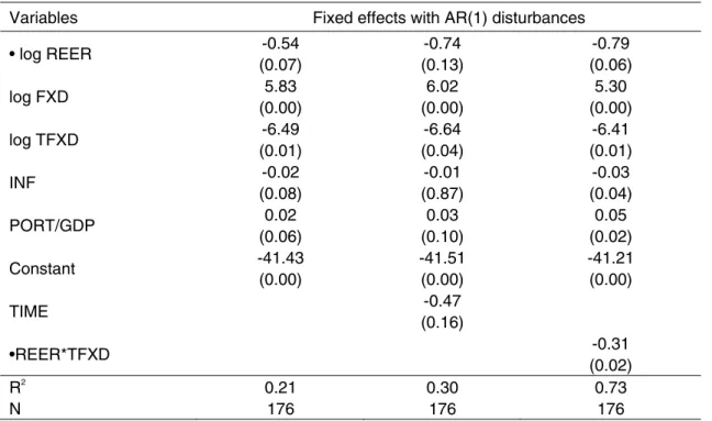
Equation (5) was estimated by (within-groups) fixed and random effects to allow for country specific time invariant effects. The fixed effects (FE) model is built on an assumption that there is correlation between country specific factors (unobserved specific effects) and independent variable(s). In the presence of such correlation, FE generates consistent estimators while random effects (RE) estimation provides inconsistent coefficients of regressors. If the correlation is zero, RE estimation generates consistent and efficient estimators whilst estimators given by FE model are still consistent but inefficient (Wooldridge 2002).The Hausman test is used to justify which technique is more appropriate and, in our case, the test shows a preference for FE. However, an LM test for first-order autocorrelation of the residuals suggests the errors are not independent and identically distributed, generating inefficient estimators (Beck and Katz 1995). Consequently, fixed-effects with first-order autocorrelation disturbances estimation (Baltagi and Li 1991) in STATA is employed (to remedy this problem) and these are the estimates reported (Udomkerdmongkol et al. 2006 provide other results). Results for a robustness check of regional effects on FDI determination by dividing the countries into two regions, Latin America and Asia, are also reported. Table 1 reports estimated coefficients for the significant variables for net US inward FDI to emerging markets for 1990-2002. The principle variables are bilateral exchange rates adjusted for inflation (log FXD), change in log of REER (∆REER) and the temporary component of the exchange rates (log TFXD). In line with the hypotheses, the findings indicate that FDI rises when devaluation occurs (higher FXD); an expected devaluation lowers current inward FDI (negative coefficient on ∆REER); and volatile exchange rates discourage FDI (negative coefficient on TFXD). The estimated coefficients are usually statistically significant at least at the 10 per cent level (the exchange rate ‘expectation effect’ is the weakest). Inflation and portfolio investment are the only other variables with statistically significant (mostly) estimates (results from estimating the full model are reported in Appendix Table B1), and of the expected signs: a rise in foreign investor’s confidence and lower inflation in a host country stimulate inflows of FDI. The results are broadly consistent with prior expectations and with the evidence found in previous studies of FDI determination such as Schneider and Frey (1985) and Tuman and Emmert (1999).
To test the hypothesis that the 1997 economic crisis may decrease inflows of FDI to emerging markets as found in Siamwalla (2004), we include a time dummy variable (TIME), which equals to 1 if the period is 1997-2002 and 0 otherwise (second column of results). Although the dummy is insignificant, the coefficients on exchange rate expectation and inflation become insignificant. One inference is that the crisis represented a large shock so foreign investors discounted the information contained in expectations and inflation, that is, disequilibrium levels of REER and inflation were considered to be consistent with a crisis period.
The interaction term (∆REER*TFXD) is included to assess if exchange rate expectations interact with volatility in influencing FDI inflows (estimates for other variables are largely unaffected). Carlson and Osler (2000) argue that speculative activities can increase exchange rate movements and so suggest a positive connection between expectations and volatility, that is, agents reacting to expectations increase volatility. On the other hand, Honohan (1984) argues that in a rumor-prone market with volatile exchange rates, agents attach less importance to their expectations and focus on
Table 1: Exchange rates and FDI, emerging markets, 1990-2002 Dependent variable: net FDI from the US
Variables Fixed effects with AR(1) disturbances • log REER -0.54 (0.07) -0.74 (0.13) -0.79 (0.06) log FXD 5.83 (0.00) 6.02 (0.00) 5.30 (0.00) log TFXD -6.49 (0.01) -6.64 (0.04) -6.41 (0.01) INF -0.02 (0.08) -0.01 (0.87) -0.03 (0.04) PORT/GDP 0.02 (0.06) 0.03 (0.10) 0.05 (0.02) Constant -41.43 (0.00) -41.51 (0.00) -41.21 (0.00) TIME -0.47 (0.16) •REER*TFXD -0.31 (0.02) R2 0.21 0.30 0.73 N 176 176 176
Notes: Figures in parentheses are P-values; the first two columns of results included all explanatory variables, the final column includes only significant coefficients (see Appendix Table B1).
‘following the market’ so there will be a negative relationship between expectations and volatility. Including the interaction term improves the overall performance of the regression (R2 = 0.73 for the parsimonious specification), and the coefficient is negative and statistically significant. If devaluation is expected (∆REER > 0), volatility and expectations lower FDI (the interaction adds to the discouraging effect of each alone). The case of expected appreciation (∆REER < 0) is more complicated: the expectation itself encourages FDI, while volatility discourages FDI. The two interact so only if the change in REER is between 0 and -25 does the negative volatility effect outweigh the positive expectations.8 This is a large range so the negative volatility effect will usually dominate, a finding that is broadly consistent with Cushman (1985, 1988) and Goldberg and Kolstad (1995).
The separate exchange rate effects on FDI may differ across regions. The 1997 economic crisis had a major direct impact on exchange rates in Asian countries (Siamwalla 2004), especially as the crisis implied that some countries abandoned a hard peg exchange rate regime. To test for regional effects on US FDI equation (5) is expanded to include a dummy variable for Asian countries interacted with the core explanatory variables.
FDIi,t = β0 +β Δ1 REERi,t + β2FXDi,t + β3TFXDi,t+ β4Xi,t+β5ASIA +
β6 ASIA*ΔREERi,t + β7 ASIA*FXDi,t +β8 ASIA*TFXDi,t+ µi + εi,t (6)
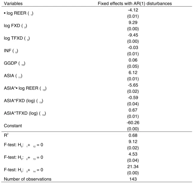
where ASIA is a dummy variable that is 1 for Asian countries and 0 otherwise. For easier interpretation only Latin American countries are also included in the sample (the African countries are omitted). Table 2 reports the results for the parsimonious specification (significant variables only). In Appendix Table B2 fixed effects results are included for comparison, and are broadly consistent; as the tests suggest misspecification due to first-order autocorrelation9 we concentrate on results for fixed-effects with AR(1) disturbances (Udomkerdmongkol et al. 2006 provide other results).
Table 2: US FDI to emerging markets: is Asia different?
Dependent variable: net FDI from the US
Variables Fixed effects with AR(1) disturbances • log REER ( 1) -4.12 (0.01) log FXD ( 2) 9.29 (0.00) log TFXD (3) -9.45 (0.00) INF ( 5) -0.03 (0.01) GGDP ( 10) 0.06 (0.05) ASIA ( 11) 6.12 (0.01) ASIA*• log REER ( 12)
-5.65 (0.02) ASIA*FXD (log) ( 13) -0.59 (0.04) ASIA*TFXD (log) (14) 0.67 (0.01) Constant -60.26 (0.00) R2 0.68 F-test: H0: 1+ 12 = 0 9.12 (0.02) F-test: H0: 2+ 13 = 0 4.53 (0.04) F-test: H0: 3+ 14 = 0 21.34 (0.00) Number of observations 143
Notes: Figures in parentheses are P-values; only variables with significant coefficients are included (full results in Appendix table B2). The F-test shows that regional dummies are all important (reject the null of joint coefficients = 0).
9 The LM test statistic is greater than the 5 per cent critical value of the chi-squared distribution with 1 degree of freedom so we can reject the null hypothesis of no first-order autocorrelation. The Koenker-Bassett test statistic shows that the errors are homoscedastic.
The coefficients on the ASIA dummy and interaction terms are instructive. On average, Asian countries receive about US$3 billion more FDI from the US than Latin American countries.10 In Latin America, the effect of an expected devaluation (increasing REER) is –4.0, but for Asian countries it is –9.77 (that is, β1 + β12). Expectations of devaluation appear to have a much greater effect in discouraging (postponing) US FDI in Asian countries. This may be because many Asian economies at exchange rates pegged to the US dollar so an expected devaluation implied abandoning the peg (that is, a currency crisis).
In contrast, the impacts of volatile exchange rates and the value or level of the local currency are just slightly weaker for Asian countries (the differences are significant, but small). In general, for Latin American and Asian countries (and the three African countries by implication from Table 1), the impacts of separate exchange rate indicators are similar, except for expectations. US FDI to Asia appears significantly higher than to other regions but is more susceptible to expected devaluation, probably because this indicates a currency crisis is likely (and investors will wish to withdraw from the market before the crisis and devaluation occur).
In addition to the exchange rate variables, inflation and market potential (GGDP) are the only significant variables: inflation discourages FDI whereas market potential encourages inflows of FDI. Compared to Table 1, an interesting result is that portfolio investment is no longer significant, suggesting that this measure of investor confidence was important in explaining flows to Asia relative to Latin America, an effect accounted for by the Asia intercept term in Table 2. Once regional differences are accounted for, GDP growth is a significant indicator of the attractiveness of a country for US FDI. It may previously have been insignificant to the extent that Asian growth performance was superior to Latin America.
5 Concluding remarks
This paper investigates the effects of exchange rates, exchange rate expectations, and exchange rate volatility on (net) US FDI to 16 emerging market countries over 1990-2002. The empirical approach is motivated by the model of Chakrabarti and Scholnick (2002) and three hypotheses: a cheaper local currency (current devaluation) stimulates inward FDI; expectations of local currency devaluation (appreciation) encourage postponing (bringing forward) FDI; and exchange rate volatility discourages FDI inflows.
The results can be summarized as:
1. Foreign investors look to markets where their money can buy more. There is robust evidence the value of the local currency is associated with FDI inflows: a current devaluation (appreciation) increases (decreases) FDI inflows in that year.
10 Expected FDI to Asia is represented by ∂FDI / ∂ASIA = β11 + β12ΔREER+ β13FXD+β14TFXD =
2. Foreign investors will postpone FDI if they expect local currency depreciation, but may bring forward FDI if they expect an appreciation. Investors consider not only the current value of a local currency but also the likely movements in that currency in the near future in deciding on the location and timing of FDI.
3. There is evidence for a negative effect of exchange rate volatility on FDI inflows. Foreign investors are deterred by volatility because it represents uncertainty over the value of their investment.
4. There is only limited evidence that economic conditions and foreign investors’ confidence in host countries are significant determinants of US FDI. It may be that investors treat emerging markets as quite similar in terms of potential and hence attach greatest weight to exchange rate (price) variables.
5. The 1997 economic crisis itself had no clear impact on US FDI in emerging markets, possibly because the impact was through exchange rates, especially in Asia, which then affect FDI. The result that an expected devaluation had a much greater deterrent effect on FDI for Asia than for Latin America is consistent with this, as expected devaluation in Asia is a signal that a crisis (abandoning the hard peg) is expected.
Foreign investors in emerging markets do respond to the exchange rate: devaluation attracts FDI (as it reduces the price of assets abroad), although an expected devaluation postpones FDI. The expectation effect is consistent with FDI being undertaken to service domestic demand for finance, telecommunications, wholesaling and retailing rather than to tap cheap labour (IMF 2003). US investors are discouraged by volatile exchange rates, perhaps because this is correlated with economic and political uncertainty, which also appears to discourage FDI. There is also an additional interaction effect between expectations and volatility: the adverse effect of expected devaluation is attenuated by volatility, whereas the benefit of expected appreciation is dampened by volatility. This is consistent with cautious investors if volatility is interpreted as an indicator of the reliability of expectations – they are more concerned with potential downside effects (future devaluation) than upside benefits (future appreciation). Thus, in general volatility is a more important signal to investors (FDI is more responsive) than expected devaluation, but in Asian economies (many of which operated a hard peg to the US dollar) expected devaluation has an attenuated effect as a signal of anticipated crisis.
Our analysis contributes to the discussion of the impacts of exchange rates on FDI. However, the sample is limited to relatively few countries, and we were unable to avail of data from futures exchange rate markets or high frequency (monthly or daily) exchange rate data. The analysis is also limited to the extent that MNEs have different FDI objectives. Suppose two types of MNEs exist in a host country: one is interested in low cost production (export-oriented FDI) but the other is interested in domestic sales (market-seeking FDI). Aggregate (country-level) analysis cannot identify differential responses of these MNEs to exchange rate indicators; such investigation requires firm-level analysis. Nevertheless, the analysis illustrates the importance of maintaining a relatively stable exchange rate to attract FDI.
References
Asiedu, E. (2002). ‘On the Determinants of Foreign Direct Investment to Developing Countries: Is Africa Different?’. World Development, 30(1): 107–119.
Baltagi, B. H., and Q. Li (1991). ‘A Transformation that will Circumvent the Problem of Autocorrelation in an Error-component Model’. Journal of Econometrics, 48: 385–93.
Baum, C. F. (2006). An Introduction to Modern Econometrics Using STATA. Texas: STATA Press.
Beck, N., and J. N. Katz (1995). ‘What to do (and not to do) with Time-series Cross-section Data’. American Political Science Review, 89: 634–37.
Blonigen, B. A. (1997). ‘Firm – Specific Assets and the Link between Exchange Rates and Foreign Direct Investment’. American Economic Review, 87: 447–65.
Bond, S. (2002). ‘Dynamic Panel Data Models: A Guide to Micro Data Methods and Practice’. Cemmap Working Paper CWP09/02. The Institute for Fiscal Studies. Bureau of Economic Analysis (2004). US-International Transactions Account Data.
Available from http://www.bea.gov/bea/di1.htm/.
Busse, M., and C. Hefeker (2005). ‘Political Risk, Institutions and Foreign Direct Investment’. HWWA Discussion Paper No. 315, (HWWA) Institute of International Economics.
Campa, J. M. (1993). ‘Entry by Foreign Firms in the United States under Exchange Rate Uncertainty’. Review of Economics and Statistics, 75: 614–22.
Carlson, J. A., and C. L. Osler (2000). ‘Rational Speculators and Exchange Rate Volatility’. European Economic Review, 44: 231–53.
Chakrabarti, R., and B. Scholnick (2002). ‘Exchange Rate Expectations and Foreign Direct Investment Flows’. Weltwirtschaftliches Archiv, 138(1): 1–21.
Chinn, M. D. (2005). ‘A Primer on Real Effective Exchange Rates: Determinants, Overvaluation, Trade Flows and Competitive Devaluation’. NBER Working Paper No. 11521, National Bureau of Economic Research.
Cohen, D. (1991). ‘Slow Growth and Large LDC Debt in the Eighties: An Empirical Analysis’. CEPR Discussion Paper No. 461, Center for Economic Policy Research. Cushman, D. O. (1985). ‘Real Exchange Rate Risk, Expectations, and the Level of
Direct Investment’. Review of Economics and Statistics, 67: 297–308.
Cushman, D. O. (1988). ‘Exchange – Rate Uncertainty and Foreign Direct Investment in the United States’. Weltwirtschafiliches Archiv, 67: 297–308.
Frankel, J., and K. Froot (1987). ‘Using Survey Data to Test Standard Propositions RegardingExchangeRateExpectations’.American Economic Review, 77(1): 133–53. Froot, K., and J. Stein (1991). ‘Exchange Rates and Foreign Direct Investment: An
Imperfect Capital Markets Approach’. Quarterly Journal of Economics, 196: 1191– 1218.
Gastanaga, V. M., J. B. Nugent, and B. Pashamova (1998). ‘Host Country Reforms and FDI Inflows: How Much Difference do they Make?’. World Development, 26(7): 1299–1314.
Goldberg, L. S., and C. D. Kolstad (1995). ‘Foreign Direct Investment, Exchange Rate Variability and Demand Uncertainty’. International Economic Review, 36: 855–73. Goldberg, L. S., and M. Klein (1998). ‘Foreign Direct Investment, Trade and Real
Exchange Rate Linkages in Developing Countries’. In R. Glick (ed.), Managing Capital Flows and Exchange Rates: Perspectives from the Pacific Basin. Cambridge: Cambridge University Press: pp. 73–100.
Goldfajn, I., and R. O. Valdés (1999). ‘The Aftermath of Appreciations’. The Quarterly Journal of Economics, 114(1): 229–62.
Hodrick, R., and E. Prescott (1997). ‘Post-war US Business Cycles: An Empirical Investigation’. Journal of Money Credit and Banking,29: 1–16.
Honohan, P. (1984). ‘Expectation Errors and Exchange-Rate Volatility’. Journal of Macroeconomics,6(3): 323–34.
International Monetary Fund (2003). ‘Foreign Direct Investment in Emerging Market Countries’. Report of the Working Group of the Capital Markets Consultative Group, International Monetary Fund.
Klein, M. W., and E. S. Rosengren (1994). ‘The Real Exchange Rate and Foreign Direct Investment in the United States: Relative Wealth vs. Relative Wage Effects’. Journal of International Economics, 36: 373–89.
Lipsey, R. E. (2001). ‘Foreign Direct Investors and the Operations of Multinational Firms: Concepts, History and Data’. NBER Working Paper No. 8665, National Bureau of Economic Research.
Neumayer,E.,and L. Spess(2005). ‘Do BilateralInvestment TreatiesIncreaseForeign DirectInvestmenttoDevelopingCountries?’.WorldDevelopment,33(10): 1567–585. Newbold, P. (1995). Statistics for Business and Economics, 4th edn. New Jersey:
Prentice-Hall, Inc.
Schneider, F., and B. S. Frey (1985). ‘Economic and Political Determinants of Foreign Direct Investment’. World Development, 13(2): 161–75.
Siamwalla, A. (2004). ‘Anatomy of the Crisis’. In P. G. Warr (ed.) Thailand Beyond the Crisis (Rethinking South East Asia). Routledge: London.
Singh, H., and K. W. Jun (1995). ‘Some New Evidence on Determinants of Foreign Direct Investment in Developing Countries’, Policy Research Working Paper No. 1531,The World Bank.
Tuman, J. P., and C. F. Emmert (1999). ‘Explaining Japanese Foreign Direct Investment in Latin America, 1979-1992’. Social Science Quarterly, 80(3): 539–55.
Udomkerdmongkol, M., H. Görg, and O. Morrissey (2006). ‘Foreign Direct Investment and Exchange Rates: A Case Study of US FDI in Emerging Market Countries’. University of Nottingham, School of Economics, Discussion Paper 06/05
Wheeler, D., and A. Mody (1992). ‘International Investment Location Decisions’.
Journal of International Economics, 33: 57–6.
Wooldridge, J. M. (2002). Econometric Analysis of Cross Section and Panel Data. London: MIT Press.
World Bank (2004). World Development Indicators 2004. Available from http://devdata.worldbank.org/dataonline/.
Appendix A: Data and sources
The independent variables are measured as:
1. Real effective exchange rate indices (REER, 2000 = 100) from IMF International Financial Statistics. The IMF defines the REER as nominal effective exchange rate11 (NEER) adjusted for relative movements in national price indicators (CPI) of a home country and selected countries.
2. Average official bilateral exchange rates (local currency unit against US dollar) are from World Development Indicators (WDI 2004). They are adjusted by CPI (2000 = 100) of host countries to acquire real exchange rates (Cushman 1985, 1988; Froot and Stein 1991; Klein and Rosengren 1994).
3. Manufacturing (MNU) as a share of GDP (constant 2000, US dollar) is from WDI 2004 as a proxy for industrialization (Wheeler and Mody 1992).
4. Inflation (INF), measured as percentage annual growth of the GDP deflator, is from WDI 2004 as a proxy of macroeconomic conditions (Schneider and Frey 1985; Tuman and Emmert 1999).
5. Exports of goods and services (EXP) as a ratio of GDP (constant 2000, US dollar) is from WDI 2004 as a proxy of export potential (Singh and Jun 1995; Aseidu 2002).
6. GDP per capita (PGDP; constant 2000, US dollar) is from WDI 2004 as a proxy of labour costs (Cohen 1991). While this is admittedly a rough proxy it may not be too problematic in our cross-country context, where differences in labour costs across country can be expected to be highly correlated with differences in GDP per capita.
7. Portfolio investment (current, US dollar) is from WDI 2004. It is adjusted by GDP (current, US dollar) to obtain portfolio investment (PORT/GDP) as a proxy of foreign investors’ confidence.
8. Data on number of telephone mainlines (TEL) extracted from WDI 2004, as a proxy for infrastructure (Aseidu 2002).
9. GDP growth (GGDP; constant 2000, US dollar) is from WDI 2004, used as a proxy of market potential (Gastanaga et al.1998; Neumayer and Spess 2005). Tables A1 and A2 provide descriptive statistics for and correlations between these variables.
11 The IMF defines NEER as a ratio of period average exchange rates currency in question (index) to a trade weighted geometric average of exchange rates for selected country currencies.
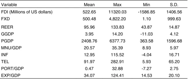
Table A1: Descriptive statistics
Sample: 16 countries and 1990-2002
Variable Mean Max Min S.D.
FDI (Millions of US dollars) 522.65 11320.03 -1586.85 1406.56
FXD 500.48 4,822.20 1.10 999.63 REER 95.96 133.83 43.87 14.87 GGDP 3.95 14.20 -11.03 4.12 PGDP 2408.76 6377.73 363.58 1596.68 MNU/GDP 20.57 35.39 8.93 5.97 INF 12.95 115.52 -4.04 16.71 TEL 91.97 282.91 5.93 65.20 PORT/GDP 0.47 32.88 -7.27 2.75 EXP/GDP 34.07 124.41 14.53 20.10
Source: US Department of Commerce, WDI 2004 and the author’s computation.
Table A2: Correlation matrix
Sample: 16 countries and 1990-2002
FDI •REER FXD TFXD GGDP PGDP MNU/GDP INF TEL PORT/GDP EXP/GDP
FDI 1 •REER 0.19 1 FXD 0.25 0.07 1 TFXD -0.02 -0.19 0.04 1 GGDP 0.12 0.31 -0.18 -0.25 1 PGDP 0.25 0.12 0.21 -0.04 -0.15 1 MNU/GDP -0.02 -0.02 -0.37 0.05 0.38 -0.15 1 INF 0.30 0.13 0.33 0.16 -0.15 0.33 -0.18 1 TEL 0.08 0.03 0.08 -0.01 -0.13 0.86 -0.01 0.13 1 PORT/GDP 0.03 0.12 0.01 -0.21 -0.03 -0.02 -0.03 0.04 -0.08 1 EXP/GDP -0.01 0.11 0.28 0.08 0.12 0.26 0.45 -0.21 0.21 -0.18 1
Appendix B: Full econometric results
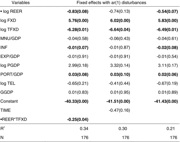
Table B1: Exchange rates and FDI, emerging markets, 1990-2002
Dependent variable: net FDI from the US
Variables Fixed effects with ar(1) disturbances
• log REER -0.83(0.08) -0.74(0.13) -0.54(0.07) log FXD 5.76(0.00) 6.02(0.00) 5.83(0.00) log TFXD -6.28(0.01) -6.64(0.04) -6.49(0.01) MNU/GDP -0.04(0.58) -0.06(0.43) -0.04(0.61) INF -0.01(0.07) -0.01(0.87) -0.02(0.08) EXP/GDP -0.01(0.91) -0.01(0.91) -0.01(0.54) log PGDP 2.99(0.18) 3.32(0.14) 3.11(0.17) PORT/GDP 0.03(0.08) 0.03(0.10) 0.02(0.06) log TEL -0.65(0.21) -0.41(0.44) -0.67(0.19) GGDP 0.01(0.83) 0.01(0.95) 0.01(0.89) Constant -40.33(0.00) -41.51(0.00) -41.43(0.00) TIME -0.47(0.16) •REER*TFXD -0.25(0.04) R2 0.34 0.30 0.21 N 176 176 176
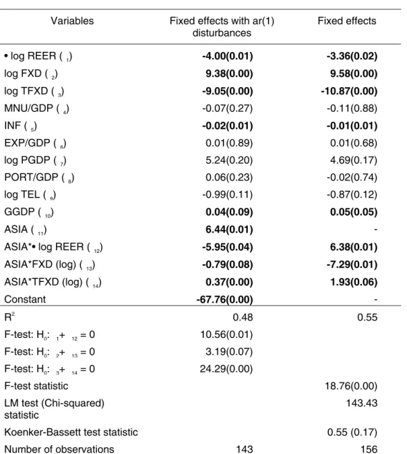
Table B2: US FDI to emerging markets: is Asia different?
Dependent variable: net FDI from the US
Variables Fixed effects with ar(1) disturbances Fixed effects • log REER (1) -4.00(0.01) -3.36(0.02) log FXD ( 2) 9.38(0.00) 9.58(0.00) log TFXD (3) -9.05(0.00) -10.87(0.00) MNU/GDP (4) -0.07(0.27) -0.11(0.88) INF (5) -0.02(0.01) -0.01(0.01) EXP/GDP (6) 0.01(0.89) 0.01(0.68) log PGDP (7) 5.24(0.20) 4.69(0.17) PORT/GDP (8) 0.06(0.23) -0.02(0.74) log TEL (9) -0.99(0.11) -0.87(0.12) GGDP ( 10) 0.04(0.09) 0.05(0.05) ASIA (11) 6.44(0.01) -
ASIA*• log REER ( 12) -5.95(0.04) 6.38(0.01)
ASIA*FXD (log) (13) -0.79(0.08) -7.29(0.01) ASIA*TFXD (log) (14) 0.37(0.00) 1.93(0.06) Constant -67.76(0.00) - R2 0.48 0.55 F-test: H0: 1+ 12 = 0 10.56(0.01) F-test: H0: 2+ 13 = 0 3.19(0.07) F-test: H0: 3+ 14 = 0 24.29(0.00) F-test statistic 18.76(0.00) LM test (Chi-squared) statistic 143.43
Koenker-Bassett test statistic 0.55 (0.17)
Number of observations 143 156
Notes: Figures in parentheses are P-values (significant coefficients in bold). The Koenker-Bassett test for heteroscedasticity is passed (accepts the null of homoscedastic error). The LM test indicates autocorrelation in the FE so FE with AR(1) error is appropriate (the 5% critical value of Chi-squared distribution with 1 degree of freedom is 3.84). The F-test shows that regional dummies are all important (reject the null of joint coefficients = 0).