E
ffi
cient 3D object recognition using foveated point clouds
Rafael B. Gomes, Bruno M. F. Silva, Lourena Rocha, Rafael V. Aroca, Luiz Velho, Luiz M. G. Gonc¸alves
Abstract
Recent hardware technologies have enabled acquisition of 3D point clouds from real world scenes in real time. A variety of interactive applications with the 3D world can be developed on top of this new technological scenario. However, a main problem that still remains is that most processing techniques for such 3D point clouds are computationally intensive, requiring optimized approaches to handle such images, especially when real time performance is required. As a possible solution, we propose the use of a 3D moving fovea based on a multiresolution technique that processes parts of the acquired scene using multiple levels of resolution. Such approach can be used to identify objects in point clouds with efficient timing.Experiments show that the use of the moving fovea shows a seven fold performance gain in processing time while keeping 91.6% of true recognition rate in comparison with state-of-the-art 3D object recognition methods.
Keywords: point cloud, 3D object recognition, moving fovea
1. Introduction
1
With current developments experienced in hardware
tech-2
nologies, computer vision systems would be ideally able to
3
capture 3D data of the world and process this data in order to
4
take advantage of their inherent depth information. However,
5
nowadays, most current computer vision systems are still based
6
on 2D images while the use of 3D data can offer more details
7
about geometric and shape information of captured scenes and
8
consequently, of general objects of interest. In this way, the
de-9
velopment of 3D object recognition systems has been an active
10
research topic over the last years [1].
11
Recent technology advances have enabled the construction of
12
devices, as for example the Microsoft Kinect [2], that capture
13
3D data from the real world. The Kinect is a consumer grade
14
RGB-D sensor originally developed for entertainment that has
15
enabled several novel works for research including robotics,
16
commercial, and gaming applications. Mobile phone
manu-17
factures have also started to shipping smartphones with stereo
18
vision cameras in the recent years. Other manufacturers
al-19
ready announced camera sensors with depth information as a
20
4th channel. Furthermore, the price reduction of equipment is
21
driving a wide adoption of 3D capture systems.
22
Although the amount of data provided by 3D point clouds is
23
very attractive for object recognition, it requires intensive
com-24
puting algorithms that could render systems based on this type
25
of data computationally prohibitive, mainly if real time
inter-26
action is needed. Hardware accelerators and optimizations are
27
frequently used for real time computing, however object
recog-28
nition is still an open research field with several challenging
29
research opportunities, especially when real time performance
30
is desired. One software solution consists in processing point
31
clouds efficiently using algorithms that compute local
geomet-32
ric traits. One example of such system is depicted in Section
33
4, which enumerates advantages of correspondence grouping
34
algorithms.
35
We are interested on accelerating object retrieval using 3D
36
perception tools and data acquisition from real images (not
syn-37
thetic images). For this purpose, we propose the usage of a
38
moving fovea approach to downsample 3D data and reduce the
39
processing of the object retrieval system from point clouds. An
40
example of foveated cloud can be seen in Figure 1.
Experimen-41
tal results show that our system offers up to seven times faster
42
recognition time computing without compromising recognition
43
performance. We also provide two web based tools to
interac-44
tively view and manipulate point clouds and to capture Kinect
45
point clouds without the need to install any software, which has
46
been used within the Collage Authoring System.
47
This article is structured as follows: Section 2 presents the
48
theoretical background used in this work with reviews of some
49
related works on 3D object retrieval and the moving fovea
ap-50
proach. Section 3 describes 3D moving fovea applied to the
51
object recognition problem and its formulation in the context of
52
our work. Section 4 depicts both the system that forms the base
53
of our implementation and also the proposed scheme, along
54
with implementation considerations. Section 5 describe the
ex-55
periments, including a performance evaluation that can be
exe-56
cuted with the Collage authoring environment, while Section 6
57
closes the article with our final remarks.
58
2. Theoretical Background
59
Three-dimensional object recognition is a multi-disciplinary
60
area of research, with major contributions originating from the
61
Pattern Recognition, Computer Vision, Robotics and Computer
62
Graphics communities. In this Section, relevant contributions
63
from each of these subareas are briefly enumerated,
emphasiz-64
ing the data acquisition method employed in each of them.
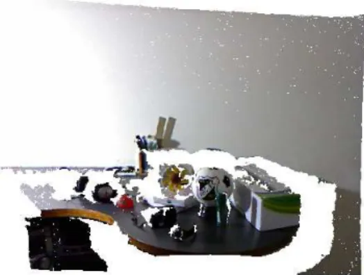
Figure 1: Example of an original point cloud and object detection in the foveated cloud
2.1. 3D Multiresolution Approaches
66
Vision is so far the most important sensing resource for
67
robotics tasks that can be executed based on devices like web
68
cameras and depth sensors. Unfortunately, the huge amount of
69
data to be processed is limited by the processing time that is a
70
restriction for doing reactive robotics. Several approaches
rep-71
resent image with non-uniform density using a foveated model
72
that mimics the retina mapping to the visual cortex in order to
73
deal with this amount of data [3, 4, 5, 6, 7, 8, 9]. The fovea is
74
the area of retina with greatest visual acuity, so foveated models
75
have high resolution nearby the fovea and decrease the
resolu-76
tion according to the distance from the fovea.
77
The foveation process is performed either by subsampling in
78
software [3, 4], by hardware with reduced sampling [10] or by
79
using a system with 2 or more cameras, where one is used for
80
peripheral vision and another one is used for foveated vision
81
[11, 12]. The software foveation allows greater ease of
modifi-82
cation and easily implementable in conventional hardware, but
83
are slower than hardware solutions which are usually more
ex-84
pensive and difficult to change. In terms of coverage, solutions
85
that use specific cameras to peripheral and foveated vision are
86
more open to stimuli of the whole environment by using a wide
87
angle peripheral camera, what would require a huge resolution
88
camera in the case of a single camera system due to high
res-89
olution fovea needs. However, a camera specific for foveated
90
vision requires movement of physical devices and a large
dif-91
ference between peripheral and fovea cameras suppress stimuli
92
appearing on a intermediate level of resolution because these
93
are not in the fovea camera field of view neither in the
periph-94
eral camera. In this work, the foveation is performed by
soft-95
ware. It is important to note that most of these models allow
96
free movement of the fovea, what does not happen at the
bio-97
logical eye’s retina. Otherwise, all the vision resources should
98
be moved in order to keep the object at foveal region.
99
In a dynamic and cluttered world, all information needed to
100
perform complex tasks are not completely available and not
101
processed at once. Information gathered from a single eye
fixa-102
tion is not enough to complete these tasks. In this way, in order
103
to efficiently and rapidly acquire visual information, our brain
104
decides not only where we should look but also what is the
se-105
quence of fixations [13]. This sequence of fixations, and
there-106
fore the way the fovea is guided, is related to cognition
mech-107
anisms controlled by our visual attention mechanism. Several
108
works proposes saliency maps from which fixations can be
ex-109
tracted [14].
110
It is also known that the human vision system has two major
111
visual attention behaviors or dichotomies [15]. In the top-down
112
attention approach, the task in hand guides attention
process-113
ing. On the other hand, in bottom-up attention, external stimuli
114
drive attention. Text reading is an example of the top-down
115
behavior of attention, where visual fixations are done
system-116
atically, passing through the paper in a character by character
117
and line by line movement. On the opposite, if a ball is thrown
118
toward the same reader, this bottom-up stimulus will make the
119
reader to switch attention to the dangerous situation.
120
Besides in robotic vision, several foveated systems are
pro-121
posed in order to reduce the amount of data to be coded/decoded
122
also in real-time video transmission [8, 6]. In this kind of
appli-123
cation, an image should be encoded with foveation thus keeping
124
higher resolution in regions of interests. In a similar way, Basu
125
[16] proposes a foveated system to 3D visualization with
lim-126
ited bandwidth restriction, where the fovea position controls the
127
objects’ texture quality and resolution.
128
2.2. 3D Object Recognition
129
Early object recognition systems acquired data from
expen-130
sive and rarely available range sensors, such as laser scanners
131
[17, 18] and structured light patterns [19]. Ashbrook et al. [17]
132
describe an object recognition system that relies on similarities
133
between geometric histograms extracted from the 3D data and
134
the Hough Transform [20]. Johnson and Hebert popularized the
135
Spin Images descriptor [18, 19], which was used as the basis
136
to an object recognition algorithm that groups correspondences
137
of Spin Images extracted in a given query model and those
ex-138
tracted in the scene data that share a similar rigid transformation
139
between the model and the scene [18]. Data from 3D scanners
140
and also from synthetic CAD 3D models are employed in the
141
work of Mian et al. [21].
Until recently, 3D object recognition systems processed data
143
mostly in an off-line fashion, due to long computing times
in-144
volved [22]. This paradigm has started to shift as algorithms
145
have been proposed in the Robotics community [23, 24] to
146
enable real-time manipulation and grasping for robotic
ma-147
nipulators. In fact, algorithms designed to describe 3D
sur-148
faces through histograms of various local geometric traits
eval-149
uated on point clouds became a major trend in the last years
150
[25, 26, 23, 27]. Consequently, faster and more accurate 3D
151
object recognition systems based on keypoint matching and
de-152
scriptors extracted in the scene and in the sought object point
153
clouds were developed. After being established, point
cor-154
respondences are grouped by hypotheses sharing a common
155
transformation, which is estimated by voting [28, 29],
multi-156
dimensional clustering [30, 31] or RANSAC [32] (also used to
157
detect shapes on 3D data [33]). The presence of the object of
158
interest is then inferred if certain conditions are met, such is
159
the number of votes, cluster size, or the number of RANSAC
160
inliers.
161
With the wider availability of consumer-grade depth
sen-162
sors such as the Microsoft Kinect, several works on 3D
ob-163
ject recognition are proposed employing this class of sensor
164
[34, 35, 24, 36, 37, 38]. Aldoma et al. [24] proposed the global
165
feature coined Clustered Viewpoint Feature Histogram (CVFH)
166
to improve performance of object recognition for robotics.
Ma-167
chine learning based approaches [37, 38] were formulated to
168
perform 3D object recognition making heavy use of depth
in-169
formation, without any computation on point clouds involved.
170
Aldoma et al. [34] highlight how algorithms that are part of
171
the Point Clouds Library (PCL) software package could be used
172
to form 3D object recognition systems based on local and global
173
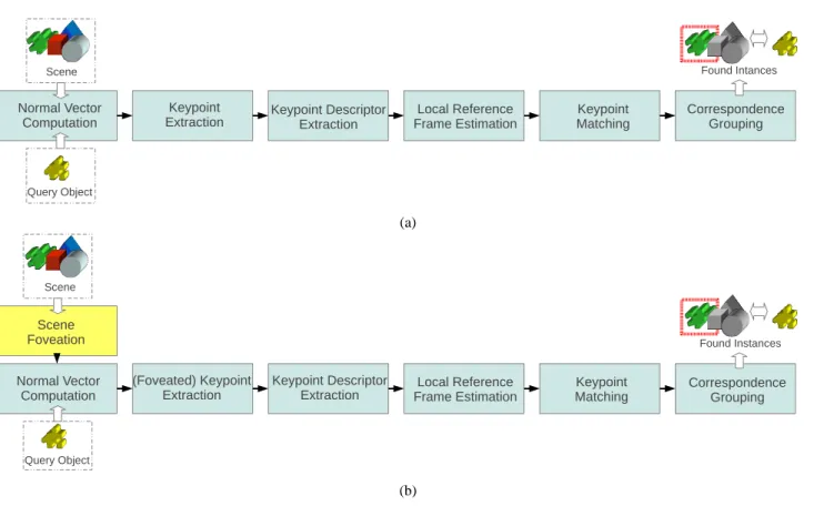
features. There are also 3D object classification/categorization
174
systems, as in the works of Wohlkinger et al. [35, 36] and of
175
Lai et al. [37]. In this latter class of systems, every chair in a
176
scene should be labeled as the object of type “chair”, whereas in
177
object recognition only the specific chair being sought should
178
be retrieved from the scene.
179
3. Foveated Point Cloud
180
This work proposes the use of a foveated point cloud in order
181
to reduce the processing time of object detection. The idea is
182
that the point density is higher nearby the fovea and that this
183
density decreases according to the distance from the fovea. In
184
this way, it is possible to reduce the total number of the points
185
reducing also the processing time at the same time that the
den-186
sity around the fovea is enough to keep feasible the object
de-187
tection. Parts of the point cloud with reduced density may be
188
useful in providing other stimuli which may be part of a
con-189
text of visual attention. For example, a saliency map can be
190
computed in the foveated cloud in order to drive bottom-up or
191
top-down stimulus. This can be very useful in the context of
192
robotic vision, since the robot can be aware to multiple
simul-193
taneous stimuli in the environment.
194
3.1. Foveated Point Cloud Model
195
The foveated point cloud proposed here is based on the 2D
196
foveated model proposed by Gomes [4]. This model transforms
197
an image into a set of smaller images with same size but with
198
different resolutions. In order to achieve that, the model defines
199
image patches from the original image that are arranged in a
200
sequence of levels. The first level is a mapping of the whole
201
original image while the last one is a mapping of a patch placed
202
at the original image centered at a fovea. This patch has the
203
same size of each image level. The result is a set of small
im-204
ages that composes a foveated image.
205
In the 3D case, instead of resampling concentric image
206
patches, the foveated point cloud is achieved by downsampling
207
the original point cloud using concentric boxes, each one
rep-208
resenting a level as shown in Figure 2. Each box specifies a
209
point cloud crop each one with a different point cloud density.
210
The outer box has one of its corners placed at a specific 3D
co-211
ordinate and it defines the model coordinate system. See the
212
red axes in Figure 2. All points outside this box are discarded.
213
Inside it, smaller boxes are linearly placed. The smallest box
214
is centered at a parameter called fovea: a 3D coordinate where
215
the point cloud density is maximum. A downsampling schema
216
is applied in this smallest box. Each bigger box are also
down-217
sampled but with a level by level decreasing point cloud density
218
up to the outer box, where the point cloud density is minimum.
219
The proposed foveated point cloud is formalized as follow.
220
We define m+1 3D boxes of size Sk∈R3, with k=0,1, ...,m
221
representing each level. Each level of the foveated point cloud
222
model changes the point cloud density. The first level (level 0)
223
has a density reduction by d0 and the last one (level m) has a
224
density reduction by dm. The density reduction of intermediate
225
levels are given by linear interpolation between d0and dm.
226
The largest box has three parameters: size (S0), orientation
227
and position (denoted by∆). Usually, if the whole point cloud
228
should be covered, it is possible to automatically set these three
229
parameters as the bounding box of the entire scene. However
230
in some applications, it could be interesting to place it in a part
231
of a huge point cloud. The last two parameters determines the
232
model coordinate system.
233
The smallest box is guided by a fovea F at that box
cen-234
ter. For formalization convenience, the fovea coordinate
sys-235
tem origin is (0,0,0) at the largest box center. In this way,
236
F=F′−S0/2, where F′is the fovea at model coordinate system.
237
Letδk∈R3be the displacement of box at level k, thenδ0 =
238
(0,0,0) andδm+Sm/2=F′.
239
The displacement of each box using linear interpolation is
240 given by: 241 δk= k(S0−Sm+2F) 2m (1) 242
Note that δk is defined only for m > 0; in other words, the
243
foveated model should have at least 2 levels.
244
The size of each k−th box using linear interpolation is given
245 by: 246 Sk=kSm−kS0+mS0 m (2) 247
x y S 0 x S 0 z S 0 y Æx 1 Æx 2 (a) x y S 0 x S 0 z S 0 y Æx1 Æx2 (b)
Figure 2: Foveated model with 3 levels. Two different placements for the fovea were used in (a) and (b).
3.2. Fovea Growth Factor
248
Here, we introduce a fovea growth factor G = (sx,sy,sz) ∈
249
R3, where s
x,sy,sz are the scale factors applied to directions
250
x, y and z, respectively (see Figure 3). As detailed in
Sec-251
tion 4, this factor increases the number of points by enlarging
252
levels volumes. Observe that this model behaves like there is
253
no foveation when G goes to∞.
254
(a) G=(0, 0, 0) (b) G=(20, 20, 20)
(c) G=(40, 40, 40) (d) G=(60, 60, 60)
Figure 3: Different values for the fovea growth factor. In this way, each level is bounded by the lower limit of
max-255
imum betweenδk−G and (0,0,0) and the upper limit of the
256
minimum betweenδk+Sk+G and S0. These minimum and
257
maximum limit the levels to the original point cloud boundary.
258
3.3. Downsampling
259
After foveated levels boundaries computation, the point
260
cloud is downsampled in order to change the point cloud
den-261
sity. In this step, there are two possibilities of point cloud
stor-262
age: to create a single point cloud joining all the
downsam-263
pled points from each level or to store each downsampled point
264
cloud from each level independently. Note that both ways can
265
be adopted simultaneously.
266
However, by joining all points in a single cloud leads to
ge-267
ometric distortions, probably imperceptible on a visual
inspec-268
tion, if the downsampling algorithm modifies the points
coordi-269
nates. A possible solution to this issue is to join all points from
270
a level that do not belong to an inner level. This way, points
271
from a level do not mix with points from another one. In order
272
to ensure the disjunction between levels, it is enough to test if
273
the point from a level k to be inserted in the foveated point cloud
274
is not inside the box k+1 (k ,m) as depicted in Algorithm 1.
275
Example of a foveated cloud point can be seen in Figure 4.
276
Input: point cloud{P}in
Input: minimum density parameter d0 Input: maximum density parameter dm
Output: point cloud{P}out
Output: point cloud vector{L}of size m+1
// Foveated Point Cloud
foreach level k do
dk=d0+k(dm−d0)/m;
downsample{P}ininto{L}kusing dkas parameter;
foreach point p of{L}kdo
if p is inside box k and is not inside box k+1 then add p to point cloud{P}out;
end end end
Algorithm 1: Processing steps applied to foveate a point
cloud.
3.4. Fovea Position
277
As explained before, one of the parameters of the foveated
278
point cloud is the fovea position vector. A dense point cloud
(a) (b) (c)
Figure 4: Example of application of the foveated model: (a) Original point cloud, (b) Foveated with m =4, Sm =(0.4,0.4,0.4),
S0=(1,1,1) and F=(−0.06,0.11,−0.75) (c) Foveated with m=4, Sm=(0.2,0.2,0.2), S0 =(1,1,1) and F=(0.05,−0.11,−0.75).
is more suitable to successful correspondence matching. If the
280
object is far from the fovea then fewer keypoints are extracted
281
and less correspondences are found. Thus, it is desirable to keep
282
the fovea near the object. In order to achieve better results, the
283
proposed architecture includes a visual attention module that
284
guides the fovea placement.
285
First, a function evaluates if the object is detected by the
sys-286
tem. If the object is detected, then the fovea is moved to the
287
object’s centroid. Otherwise, if the object is not detected, then
288
some strategy may be applied in order to recover the fovea
po-289
sition. A sequence of fixations can also be used along the time
290
or at once in order to detect where the object is. Once the object
291
is detected, a tracking module can be applied so that the fovea
292
is always in the desirable place.
293
One straight forward strategy is to disable foveation until the
294
object is found. This temporarily increases the processing time,
295
but the original point cloud is used and, then, the object can be
296
found at foveated peripheral areas. Another strategy is to
grad-297
ually increase the growth fovea factor. By using this strategy,
298
it is possible to gradually increase the number of cloud points
299
and thus avoiding having a processing time peak. Another
pos-300
sible strategy is to use a bottom-up attention strategy. In this
301
case, the fovea is moved to the most salient region, which can
302
be computed considering the class of objects to be found.
303
If the scene has more than one object, then it is possible to
304
foveate each object at a time and process them in sequence.
305
In other words, if two objects, for example, ask for top-down
306
attention, then the visual process pay attention to one in a frame
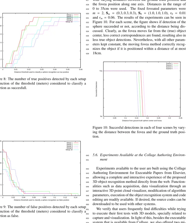
307
and to the another one in the next frame.
308
As some of these issues are not the main contribution of the
309
current work, we neglect it to be treated in a future work. We
310
just wanted to remark that it is possible to apply several
strate-311
gies based on visual attention in order to properly place the
312
fovea.
313
4. Proposed Object Recognition Scheme
314
In this section, we discuss the core framework that our
sys-315
tem is based, the correspondence grouping algorithm [29].
Af-316
ter showing the standard method, the foveated scheme to
rec-317
ognize objects is presented, along with the modifications and
318
implications that were needed to maximize performance using
319
multiresolution data.
320
4.1. Searching Objects in 3D Point Clouds
321
The proposed object recognition scheme works with point
322
clouds (set of 3D points referenced in a fixed frame)
represent-323
ing the object model and the scene to be processed. Positions
324
in this reference frame supposedly having an instance of the
325
sought object are given as outputs. We note here that our
sys-326
tem recognizes objects in a scene if and only if the model of the
327
query object is available, implying that it does not perform
ob-328
ject classification/categorization or retrieve similar objects from
329
a previously computed database (as is the case of some systems
330
enumerated on the work of Tangelder and Veltkamp [22]). Put
331
differently, the query object is searched in the scene and not
332
vice versa. As a consequence, this allows the system to find
333
multiple instances of the same object in a single scene.
334
We have chosen to build our system based on the local 3D
335
features framework, which exploits local geometric traits at key
336
positions in point clouds in order to extract discriminative
de-337
scriptors employed to establish point correspondences between
338
keypoints from the model and from the scene. These point
339
correspondences are further processed to infer possible
pres-340
ences of the object. Moreover, this class of system presents
341
some desirable and important properties, such as robustness to
342
occlusion and scene clutter, dispensing the need to elaborate
343
extensive and cumbersome training stages (mandatory for
ma-344
chine learning approaches) and ability to process point clouds
345
acquired from RGB-D sensors like the Kinect in an efficient
346
manner.
347
The system is based on the correspondence grouping
ap-348
proach of Tombari and Di Stefano [29] (with implementation
349
publicly available [39]), in which a model object is recognized
350
in the scene if, after keypoint correspondences being
estab-351
lished, enough evidence for its presence in a given position is
352
gathered. This scheme is shown in the Figure 5a. For the sake
353
of completeness, every step of the system is described as
fol-354
lows.
355
4.1.1. Extracting Local 3D Descriptors
356
The first step in the correspondence grouping algorithm is
357
to describe both the scene and model point clouds. For this,
358
the normal vector for each point is computed considering a
sur-359
face generated by a neighborhood of size knaround each point.
360
Then, a uniform downsampling algorithm is applied to extract
361
keypoints as the centroid of all points contained within a radius
362
rk. After this, SHOT (Signature of Histograms of OrienTations)
(a)
(b)
Figure 5: Object recognition algorithm based on correspondence grouping: (a) Original scheme. (b) Proposed foveated object recognition scheme. In (b), the scene is downsampled through a foveation step, reducing considerably the number of points to be processed without compromising overall accuracy (see text).
descriptors [27] are computed, assembling a histogram of the
364
normals within a neighborhood of radius rsas the signature of
365
a keypoint. The last step to fully describe point clouds is a very
366
important stage encompassing the estimation of a Local
Refer-367
ence Frame (LRF) for keypoints of the model and scene. Thus,
368
the principal axes spanning a LRF within a neighborhood of
ra-369
dius rlin each keypoint position are estimated robustly by the
370
algorithm of Petrelli and Di Stefano [40]. The result of this
371
computation (three unit vectors for each principal direction) are
372
associated with each keypoint and will be employed in the final
373
stage of the object recognition scheme. Different values for the
374
parameters are set in the scene and in the model, allowing more
375
precise recognition tasks. For clarity, the process which
ex-376
tracts descriptors for the model and scene are shown in the
Al-377
gorithms 2 and 3 respectively, with parameters knm,rkm,rsm,rlm
378
used for the model and kns,rks,rss,rlsused for the scene.
379
4.1.2. Keypoint Matching
380
For each keypoint and respective descriptor and LRF in the
381
model a match in the scene is searched by finding the closest
382
scene point (in the Euclidean sense) in the n-dimensional space
383
containing the SHOT descriptors. Search procedures are
em-384
ployed in a kd-tree to handle the cumbersome routine involved.
385
If the squared distance between the SHOT descriptors is smaller
386
than a threshold d2
max, a point correspondence is established.
387
This process is highlighted in the Algorithm 4.
388
Input: model point cloud{M} Output: model keypoint{K}m
Output: model descriptors{D}m
Output: model LRFs{L}m
// Process model
foreach point of{M}do
compute the normal vectors{N}mwithin a neighborhood of size knm;
end
from{M}, extract model keypoints{K}mby uniform downsampling with radius rkm;
foreach keypoint of{K}mdo
compute the SHOT descriptors{D}mwithin a neighborhood of size rsmusing normals{N}m; compute the set of LRFs{L}mwithin a neighborhood of size rlm;
end
Algorithm 2: Processing steps applied to the model point
cloud. See text for parameter details.
4.1.3. Correspondence Grouping
389
Since each model and scene keypoint have a LRF
associ-390
ated, a full rigid body transformation modeled by a rotation
391
and a translation can be estimated between the LRFs associated
392
with each keypoint correspondence. Accordingly, a 3D Hough
393
Space is used to gather evidence of the object presence through
Input: scene point cloud{S} Output: scene keypoint{K}s
Output: scene descriptors{D}s
Output: scene LRFs{L}s
// Process scene
foreach point of{S}do
compute the normal vectors{N}swithin a neighborhood of size kns;
end
from{S}, extract model keypoints{K}sby uniform downsampling with radius rks;
foreach keypoint of{K}sdo
compute the SHOT descriptors{D}swithin a neighborhood of size rssusing normals{N}s;
compute the set of LRFs{L}swithin a neighborhood of size rls;
end
Algorithm 3: Processing steps applied to the scene point
cloud. See text for parameter details.
Input: model and scene keypoints{K}mand{K}s
Input: model and scene descriptors{D}mand{D}s
Input: model and scene LRFs{L}mand{L}s
Output: set of keypoint correspondences{C}
initialize correspondences{C}as empty;
// Find keypoint correspondences
foreach keypoint of{K}mdo
let dmibe the descriptor of the current keypoint kmi; using{K}sand{D}s, find the nearest keypoint ks jwith descriptor ds j;
if euclidian distance(dmi,ds j)<dmaxthen add pair of triplets (kmi,dmi,lr fmi) and (ks j,ds j,lr fs j) to{C};
end end
Algorithm 4: Keypoint matching. See text for parameter
de-tails.
a voting process. After the rigid body transformation is applied,
395
the cell of the Hough Space containing this 3D position is
calcu-396
lated and its accumulator incremented. Finally, after repeating
397
these steps for all correspondences, object instances are deemed
398
found at each cell having the number of votes larger than a
pre-399
defined threshold Vh. The size of each cell is controlled by a
400
parameter Lh. The Algorithm 5 illustrates the object
recogni-401
tion scheme through correspondence grouping.
402
4.1.4. Saving Computation Time
403
We note that the normal vectors are evaluated considering
404
neighborhoods formed by all points in the clouds, whereas the
405
SHOT descriptors and LRFs are computed at the neighborhoods
406
of the keypoints. In this way, computation time is saved, while
407
the local 3D geometric traits are still kept discriminative.
408
4.2. Object Recognition in Foveated Point Clouds
409
To enhance the 3D object recognition capabilities of the
cor-410
respondence grouping approach, the cloud foveation algorithm
411
Input: Correspondences set{C} Output: set of object instances{I}
initialize Hough accumulator{H}with cell size Lh;
// Group correspondences
foreach correspondence{C}do
estimate transformation T which aligns lr fmito lr fs j; evaluate B=T kmiand find the cell h in{H}in which lies B;
increment number of votes of h;
end
foreach cell h of{H}do
if h has at least Vhvotes then
add the object instance located in the scene at h to
{I};
end end
Algorithm 5: Object recognition based on correspondence
grouping. See text for parameter details.
is employed after some adaptations. A complete scheme of the
412
proposed 3D object recognition system is shown in Figure 5b.
413
A foveated model is applied to the cloud acquired from the
414
depth sensor according to the Algorithm 1 and the parameters
415
of Table 2. Normal estimation can be done before or after
416
foveation. In the first case, the computation is more expensive,
417
but the captured geometric traits of the scene are less distorted.
418
In the current version of the system, we opted to conserve scene
419
geometry.
420
Since the keypoint extraction (uniform downsampling)
421
would extract keypoints with a single radius (originally rks),
422
the multiresolution of the scene cloud would not be respected,
423
as shows Figure 6b. Consequently, we adapted the keypoint
424
extraction to be also dependent on different and specified
lev-425
els of resolution, possibly differing of the used downsampling
426
radii d0...dm. The correspondence grouping algorithm was then
427
modified to accomodate keypoint extraction with foveated point
428
clouds. The scene points are downsampled using a different
429
radius rk for each level k = 0, ...,m. The first level (level 0)
430
uses a radius of r0 and the last (level m) uses a radius of rm.
431
All other radii from the intermediate levels are linearly
interpo-432
lated. Thus, keypoints can be extracted respecting each level of
433
the foveated scene resolution, as shows Figure 6c.
434
There are two major consequences about this approach. First,
435
there is a considerable time saving due to the keypoint
reduc-436
tion both in descriptors computation and correspondence step,
437
since different values for the extraction radius are employed
in-438
stead of a (possibly small) single value. Second, it is possible
439
to greatly increase the keypoint density near the fovea
posi-440
tion without significantly increasing the total number of
orig-441
inal scene points. This peripheral decrease and foveal increase
442
in the number of points also reduces the number of false
de-443
scriptors correspondences, improving thus the object detection
444
success rate if the fovea is properly placed.
445
In the foveated version of the recognition scheme, the
Al-446
gorithm 3 (scene processing) would be modified to include the
447
scene foveation after the normal estimation and to extract
points using a radius value rkfor each resolution level instead
449
of the rks(see Figure 5b).
450
5. Experiments and Results
451
5.1. Implementation Details
452
The proposed object recognition system is implemented in
453
C++on an Ubuntu Linux environment, making use of the
func-454
tionalities provided by the Point Cloud Library (PCL) [34]. The
455
experiments are evaluated on a non-optimized version of the
456
system running at a laptop PC with an Intel Core i5 2.5Ghz
457
processor and 4GB of RAM.
458
5.2. Ground Truth Generation
459
The availability of ground truth data allows a more in depth
460
evaluation of the proposed object recognition method by
di-461
rectly comparing the object data with the algorithm output.
462
Hence, through the use of a model object that can be described
463
analytically and also be accurately and easily identifiable on a
464
given scene, we can proceed with a more thorough analysis
re-465
garding the number of instances of the query object found and
466
its retrieved position in the scene. To cope with this, an object
467
model in the form of a sphere is utilized as ground truth after
468
some computation steps are executed in each scene to collect its
469
actual position in the global reference frame and also its radius.
470
For this, a RANSAC [41] procedure is applied aiming to fit a
471
3D sphere model in each scene point cloud. Accordingly, this
472
simple yet efficient procedure is able to correctly identify the
473
sphere in scenes with variable levels of clutter and occlusion
474
accurately enough to suffice our needs. After carefully
plac-475
ing the sphere in the scene, we manually move a Kinect sensor,
476
capturing a total of 12 frames of scenes with increasingly level
477
of clutter from different views, at the same time that the
pa-478
rameters of the detected sphere are gathered and annotated in
479
a ground truth file. Figure 7 shows 4 samples of the acquired
480
scenes and their respective ground truth.
481
5.3. Foveated Object Recognition Experiment
482
In this experiment, the correspondence grouping 3D object
483
recognition method is compared with our proposed moving
484
fovea object recognition. As can be seen in Section 4.1, the
485
standard correspondence grouping algorithm has several
pa-486
rameters which should be properly tuned according to the
op-487
eration scenario for a successful recognition procedure. This
488
can be explained because the scene/object dimensions should
489
be taken into account and also because there are not (yet)
490
any methods allowing automatically parameterization. Table 1
491
shows all parameters involved in the process and their
respec-492
tive default values. These used default values are determined
493
empirically after executing the algorithm for various scenes
494
gathered with a similar sensor (3D Kinect), setup (objects on
495
a table top) and distances between the sensor and the scene.
496
The foveated recognition scheme has parameters to be set,
497
specifying the region in 3D space and the desired resolution
498
levels. The moving fovea parameters are shown in the Table 2.
499
Desc. Def. Value
kns K-Neighbors Normals Scene 10
rks Radius Keypoints Scene 0.03
rss Radius SHOT Scene 0.02
rls Radius LRF Scene 0.015
knm K-Neighbors Normals Model 10
rkm Radius Keypoint Model 0.01
rsm Radius SHOT Model 0.02
rlm Radius LRF Model 0.015
d2
max Correspondence thresh. 0.25
Lh Size of Hough cell 0.01
Vh Voting thresh. 5
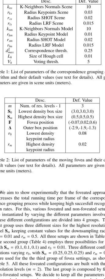
Table 1: List of parameters of the correspondence grouping al-gorithm and their default values (see text for details). All pa-rameters are given in scene units (meters).
Desc. Def. Value
m Num. of res. levels - 1 3
S0 Lowest density box size (3.0,3.0,3.0)
Sm Highest density box size (0.5,0.5,0.5)
F Fovea position (-0.07,0.02,0.6)
∆ Outer box position (-2.9,-1.9,-1.3)
r0 Lowest density 0.08
keypoint radius
rm Highest density 0.02
keypoint radius
Table 2: List of parameters of the moving fovea and their de-fault values (see text for details). All parameters are given in scene units (meters).
We aim to show experimentally that the foveated approach
500
decreases the total running time per frame of the
correspon-501
dence grouping process while keeping high succesfull
recogni-502
tion rates. For this, various foveated and non-foveated setups
503
are instantiated by varying the different parameters involved.
504
These different configurations are divided into 4 groups. The
505
first group uses three different sizes for the highest resolution
506
level Sm keeping constant values for the downsampling radii,
507
r0 =0.01 and rm=0.5. All three setups are shown in Table 3.
508
The second group (Table 4) employs three possibilities for rm
509
with Sm=(0.1,0.1,0.1) and r0 =0.01. Three different
config-510
urations varying r0, with Sm =(0.25,0.25,0.25) and rm =0.3
511
were used for the the third group of fovea settings, as shows
512
Table 5. All these foveated configurations are built with three
513
resolution levels (m= 2). The last group is composed by five
514
non-foveated setups. We decide to keep all the parameters of
515
the standard correspondence grouping constant, employing
dif-516
ferent values only for the radius to choose the scene keypoints,
517
rks. Table 6 summarizes the last group.
518
Since no object recognition methods are free of resulting in
519
false detections (false positives), some criterion to classify a
520
detection as successful (true positive) or not has to be
(a) (b) (c)
Figure 6: Keypoint extraction: (a) Foveated point cloud (b) Keypoints by uniform sampling (c) Keypoints by uniform sampling using different radii for each level.
(a) (b)
(c) (d)
Figure 7: Samples from different scene arrangements containing a sphere and the extracted sphere parameters (used as ground
truth) highlighted in wireframe. From (a) to (d), each scene has a increasingly level of clutter.
lished. To comply with this, the Euclidean distance between
522
the ground truth sphere position and the detected sphere
posi-523
tion is measured. The sphere is stated as detected if this distance
524
is below a given threshold. It is important to note that the used
525
correspondence grouping algorithm (standard and foveated) is
526
able to detect multiple instances of the same object in the scene.
527
Thus, if multiple detections are triggered within a given radius
528
around the ground truth position, only one is counted. Both
529
distance thresholds were set with a value of 8cm. The object
530
detection configurations are run in all 12 scenes with the
num-531
ber of true positives and false positives per configuration being
532
kept. There is only one instance of the sought object in each
533
scene, summing up a total of 12 true positives.
534
The results for all the 14 configurations in the 12 scenes are
535
shown in Table 7. For the first group (having varying fovea
536
size Sm), only the configurations with ID 1 and 2 were able
537
to successfully detect the object. The small fovea size (10cm
538
in each box dimension) and large rm (50cm) used in the
con-539
figuration 0 severely degrades the scene resolution to a point
540
that becomes impossible to extract relevant local features and
541
descriptors. Consequently, not enough point correspondences
542
could be stablished to detect the object.
543
Though we use the smallest fovea size of the first group in
544
all configurations of the second group, smaller values for rmare
545
set, enabling correct detections, except for the configuration 5.
546
A relatively large (14cm) for rmexplains this fact. The setup
547
number 3 detected the sphere in all 12 scenes and the setup
548
4 in only 3 of them. This is expected because a smaller rm
549
value decreases the uniform sampling radius from intermediate
550
levels (interpolated between r0and rm). Also, it increases the
551
number of keypoints throughout the levels and thus increases
552
the number of successful detections.
553
In the third group, only configuration number 6 triggered the
554
detection of the sought object in the scenes, though in not all
555
of them (11 out of 12). A larger r0was set, resulting in overly
556
downsampled point clouds and thus, no detections for setups 7
557
and 8.
558
Only the non-foveated configurations 9 and 10 detect the
ob-559
ject. This latter setup detect the sphere in all scenes without
560
any false detections, and hence can be elected the gold
stan-561
dard against which we can compare our algorithm. Curiously,
562
the configuration that results in the largest number of false
de-563
tections is the non-foveated with the highest resolution
(con-564
figuration 9) and the foveated with the largest fovea size
(con-565
figuration 2). In some sense, we could state that the overall
566
downsampling process applied by the fovea plays an important
567
role possibly removing redundancy and undesired features from
568
the scene point cloud. The largest recognition rate achieved by
569
foveated setups is also 12 true detections, but with one false
570
positive (setups 1 and 3) and two false positives (setup 2).
ID Sm r0 rm
0 (0.1,0.1,0.1) 0.01 0.5
1 (0.25,0.25,0.25) 0.01 0.5
2 (0.4,0.4,0.4) 0.01 0.5
Table 3: Group 1 of settings for the foveated recognition
-change in Sm
ID Sm r0 rm
3 (0.1,0.1,0.1) 0.01 0.02
4 (0.1,0.1,0.1) 0.01 0.08
5 (0.1,0.1,0.1) 0.01 0.14
Table 4: Group 2 of settings for the foveated recognition
-change in rm
ID Sm r0 rm
6 (0.25,0.25,0.25) 0.02 0.3
7 (0.25,0.25,0.25) 0.08 0.3
8 (0.25,0.25,0.25) 0.14 0.3
Table 5: Group 3 of settings for the foveated recognition
-change in r0 ID rks 9 0.01 10 0.02 11 0.05 12 0.08 13 0.14
Table 6: Group 4 of settings for the nonfoveated recognition -change in rks
Although the configuration number 10 has had the best
572
recognition performance in terms of detection ratio, it is the
sec-573
ond slowest of all setups, with an average of 7.201s per scene.
574
A successful recognition in the foveated scenario is achieved
575
with an average of 0.364s per frame by the setup 4, but with
576
only 0.33% of success ratio. The fastest average processing
577
time achieved (0.507s) with recognition rates higher than 50%
578
is computed by the setup 6, with 91.6% of true positive rate and
579
only 8.3% of false positive rate. This setup is also the fastest
580
showing the smallest false positive rate with at least 50% of
suc-581
cess. The setup showing the fastest computing times with true
582
positive rate at 100% is the setup 1, with an average of 1.058s
583
per frame and false positive rate of 8.3%. Of all foveated
con-584
figurations, the worst average belongs to the setup 2. In terms
585
of gain in computation performance, the fastest setup shows an
586
increase of 19.78x, while the most accurate offers 6.8x and the
587
slowest is still 2.75x faster than the better standard
correspon-588
dence grouping configuration.
589
Obviously, the slowest average computation time of all
con-590
figurations is computed with the non-foveated which has used
591
the smallest radius to extract the scene keypoints. Also, we
592
can see that as the scene resolution degrades, what is dictated
593
mainly by the two interpolating radii rather than the fovea size,
594
the computation times and recognition rate decrease.
595
ID Time (s) True False
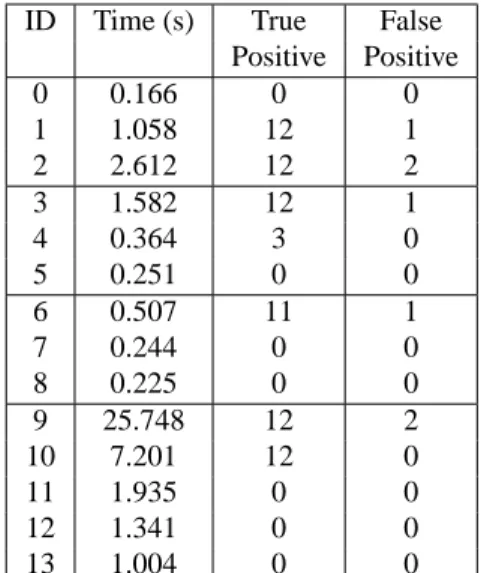
Positive Positive 0 0.166 0 0 1 1.058 12 1 2 2.612 12 2 3 1.582 12 1 4 0.364 3 0 5 0.251 0 0 6 0.507 11 1 7 0.244 0 0 8 0.225 0 0 9 25.748 12 2 10 7.201 12 0 11 1.935 0 0 12 1.341 0 0 13 1.004 0 0
Table 7: Results for a total of 14 configurations for the foveated (0-8) and non-foveated (9-13) recognition methods, after recog-nizing the ground truth objects in 12 scenes with varying levels of clutter. The average processing time is shown, along with the number of true positive detections (with distance to the true position below 0.08m).
These results emphasize that using the moving fovea, one
596
can opt to dramatically decrease recognition times providing a
597
small increase in false detections (if acceptable) or to decrease
598
recognition times keeping false detections to a minimum.
599
5.4. Detection Sensitiveness
600
Due to the criterion used in stablishing an object detection
601
as true positive and false positive, we show in Figures 8 and 9
602
how sensitive to the detection threshold (distance between the
603
detected object and the ground truth) are the best four foveated
604
setups (IDs 1, 2, 3 and 6) and the best non-foveated one (10).
605
As it can be seen in Figure 8, the best foveated setup in terms of
606
overall confiability is also the most capable to detect the object
607
closer to the ground truth position. In fact, it is even less
sensi-608
tive to the threshold than the gold standard configuration, being
609
able to recognize the object in all 12 scenes using as threshold
610
2.5cm, while the best non-foveated only recognized the same
611
number with the threshold set as 3.8cm. In the Figure 9, we
612
analyze the threshold employed to classify a detection as false
613
positive also for the top five configurations. We note that using
614
a low value (e.g. 1cm), all object detection setups find multiple
615
instances of the same object around its true position. The
non-616
foveated setup required the smallest threshold ( 4cm) to avoid
617
false detections while the setup number three was the foveated
618
configuration which required the smallest value. The most
re-619
liable foveated setup stopped triggering false detections only
620
after 13.5cm.
621
5.5. Varying the Fovea Distance to the Object of Interest
622
We also analyze how the fovea placement in the scene would
623
influence the overall object detection performance. For this,
0 2 4 6 8 10 12 0 0.01 0.02 0.03 0.04 0.05 0.06
Number of successful detections (out of 12)
Distance threshold used to classify a sphere recognition as true positive Setup 1 Setup 2 Setup 3 Setup 6 Setup 10
Figure 8: The number of true positives detected by each setup in function of the threshold (meters) considered to classify a detection as succesfull. 0 5 10 15 20 25 0 0.02 0.04 0.06 0.08 0.1 0.12 0.14
Number of false detections
Distance threshold used to classify a sphere recognition as false positive Setup 1 Setup 2 Setup 3 Setup 6 Setup 10
Figure 9: The number of false positives detected by each setup in function of the threshold (meters) considered to classify a detection as false.
we have chosen 4 samples scenes with varying amount of
clut-625
ter and run the foveated correspondence grouping algorithm
626
with varying distances between the ground truth position and
627
the fovea position along one axis. Distances in the range of
628
0 to 35cm were used. The fixed foveated parameters were
629
m = 2, Sm = (0.3,0.3,0.3), S0 = (1.0,1.0,1.0), r0 = 0.01
630
and rm = 0.06. The results of the experiments can be seen in
631
Figure 10. For each scene, the figure shows if detection of the
632
sphere succeeded or not, according to the distance being
dis-633
cussed. Clearly, as the fovea moves far from the (true) object
634
center, less correct correspondences are found, resulting also in
635
less true object detections. Nevertheless, with all other
param-636
eters kept constant, the moving fovea method correctly
recog-637
nizes the object if it is positioned within a distance of at most
638 18cm. 639 No Yes 0 0.05 0.1 0.15 0.2 0.25 0.3 0.35 Succesful Detection
Distance from ground truth sphere center and fovea Scene 1 Scene 2 Scene 3 Scene 4
Figure 10: Succesful detections in each of four scenes by vary-ing the distance between the fovea and the ground truth posi-tion.
5.6. Experiments Available at the Collage Authoring
Environ-640
ment
641
Experiments available to the user are built using the Collage
642
Authoring Environment for Executable Papers from Elsevier,
643
allowing a complete and interactive experience of the proposed
644
3D object recognition method directly from the web.
Function-645
alities such as data acquisition, data visualization through an
646
interactive 3D point cloud visualizer, modification of algorithm
647
parameters, execution of the object recognition system and code
648
editing are readily available. If desired, the source codes can be
649
downloaded to be used with other systems.
650
We verify that users frequently find difficulties while trying
651
to execute their first tests with 3D models, specially related to
652
capture and visualization. In light of this, besides the executable
653
system that is available from Collage, we also offered two
mi-654
nor contributions to this authoring environment to help users
655
to start experiment with 3D object capture and manipulation
656
quickly and easily: a data acquisition module and a tool to
ma-657
nipulate and visualize 3D point clouds.
5.6.1. Point Cloud Acquisition
659
We have developed a data acquisition module that allows
vi-660
sualization and capture of 3D point clouds using the Microsoft
661
Kinect Sensor by simply using a web browser, so users do not
662
need any specific software installed on their machine (with the
663
exception of the Kinect sensor device drivers). This system can
664
be easily used to generate 3D models of the scenes and objects
665
of interest for further processing.
666
In order to be able to capture data from the Kinect Sensor, we
667
developed a web based Kinect capture system, which relies on
668
the Java Web Start (JWS) technology to allow anyone to use it
669
with a single click on a web page. We used the OpenNI library
670
[42] and Java Native Interface (JNI) abstractions to be able to
671
connect to the Kinect sensor plugged on the user’s computer.
672
The system generates 3D point clouds in the PCD (point
673
cloud data) file format, a portable, simple and open format for
674
3D data introduced by the Point Cloud Library (PCL) [34]. It
675
consists of a standard ASCII text file containing a 3D point
in-676
formation per each line in a format separated by spaces (X Y Z
677
RGB), so any point and its color can be represented by a single
678
line of ASCII numbers.
679
5.7. Point Cloud Manipulation and Visualization
680
Another contribution is the PCD point cloud opener for
Col-681
lage. We have adapted and worked with the Collage team to
682
deploy a PCL web viewer (kindly granted to use by the PCL
683
development team) on Collage, so any Collage Experiment can
684
open and manipulate point clouds with a simple and intuitive
685
interface. The PCL viewer uses the WebGL system, a recent
686
standard for 3D object rendering directly on web pages.
We-687
bGL is supported on most modern browsers, thus, in order to
688
view and interact with the point clouds, a browser with WegGL
689
support must be used.
690
5.8. Interactive Object Recognition
691
The object recognition experiment available (Figure 11) to
692
the user in the Collage Environment is now explained in detail.
693
In order to provide his/her own input point clouds to our
ex-694
periment, users are able to use the data acquisition module
de-695
scribed in Section 5.6.1. Observe that this module is completely
696
independent from the Collage Authoring Environment.
697
Our Collage Experiment contains two experiments: Model
698
Segmentation Experiment and Object Recognition Experiment.
699
The first one is responsible for taking one point cloud
repre-700
senting a scene composed by only one object lying on a
ta-701
ble. The Model Segmentation Experiment then generates the
702
Model Point Cloud, containing only the point cloud
represent-703
ing the object. The Object Recognition Experiment takes as
704
input the Model Point Cloud generated by the previous
experi-705
ment and a point cloud of a scene containing this object, among
706
others. Then, it executes the Correspondence Grouping and the
707
Foveated Point Cloud approaches. The user is able to see the
vi-708
sual result of this execution and also text files with details about
709
it.
710
The workflow presented in the Model Segmentation
Experi-711
ment will be followed, in order to capture and segment the
ob-712
ject model (according to Sections 5.6.1 and 5.8.1 respectively).
713
A readme1.txt text file with general instructions on how to use
714
the system is available as Experiment Data Item 1, while a
715
readme2.txt (Experiment Data Item 2) explains how to proper
716
acquire and segment the object model. The scene captured
con-717
taining only the object of interest upon a table is then shown
718
in the Experiment Data Item 3, an interactive point cloud
vi-719
sualizer (see Section 5.7). Experiment Data Item 4 shows the
720
source code files. The Experiment Code Item 1 contains Bash
721
commands used to compile and execute the source code. After
722
performing the actual segmentation process, the resulting point
723
cloud containing the model data is shown in another interactive
724
window at the Experiment Data Item 5, with textual output from
725
the program shown at the Experiment Data Item 6. If desired,
726
the source code (Experiment Data Item 4) of the segmentation
727
procedure can be edited (or downloaded). In the case that the
728
user chooses not to capture data, a previously specified PCD file
729
penguin.pcd is used as default value for the Experiment Data
730
Item 3. Alternatively, a PCD file assumed to be already stored
731
in the user’s file system can also be supplied by modifying the
732
Experiment Data Item 4. We note here that this PCD file should
733
contain the object point cloud already segmented.
734
After the model acquisition and segmentation, the actual
735
Object Recognition Experiment can be executed. A text file
736
readme3.txt (Experiment Data Item 7) instructs the user on how
737
to proceed, while the source code can be visualized, edited or
738
downloaded by manipulation of the Experiment Data Item 9.
739
The user can supply a scene containing the object to be
recog-740
nized or use the default scene.pcd through the Experiment Data
741
Item 8. The experiment executes the correspondence grouping
742
algorithms in its default version (Section 4.1) and foveated
ver-743
sion (Section 4.2), resulting in two outputs presented for each
744
execution: a point cloud visualization of the recognition result,
745
highlighting the recognized instances in the scene and also the
746
object of interest and a textual output, printing important
in-747
formation of the execution such as correspondences founds and
748
execution time. These two outputs can be inspected in the
Ex-749
periment Data Item 10 and 11 (default visualization and text
750
output) and Experiment Data Item 12 and 13 (foveated
visual-751
ization and text output).
752
5.8.1. User Supplied Object Segmentation
753
In the case that the user opts to supply the object point cloud
754
via the Kinect, an object segmentation procedure has to be
ap-755
plied to the data, aiming to extract only the points belonging to
756
the object of interest. To this end, after positioning the model
757
object over a plain surface (e.g. a table) without any other object
758
on the field of view of the sensor, the point cloud is processed
759
by:
760
1. removing points that are at a distance zmaxfrom the sensor;
761
2. removing remaining points classified as contained on a plane
762
until a given fraction Fpoints of all points is reached through
763
RANSAC [41] plane segmentation;
764
3. clustering remaining points by Euclidean Distance,
imply-765
ing that starting from a single point, points with distance
766
smaller than a threshold dclusterare grouped together.
Figure 11: Workflow of the object recognition experiment available at the Collage Authoring Environment.
This simple procedure was verified experimentally to work
768
well for several objects, as can be seen in the Figures 12a and
769
12b.
770
(a) (b)
Figure 12: Algorithm showing each step of the object segmen-tation scheme, used to extract points in a scene point cloud be-longing to an object of interest. From top to bottom, left to right, the two images show the original scene, points after fil-tering by distance, points after plane removal and object points. (a) A toy car is extracted. (b) A box is segmented.
User collaboration in placing the object as indicated is
neces-771
sary to reduce the number of points to be processed and also to
772
avoid points from the object model being incorrectly discarded.
773
Some shortcomings such as incorrect point clouds as results can
774
easily be solved with proper parameter tuning.
775
6. Conclusions
776
We have presented in this article the usage of the moving
777
fovea approach to efficiently execute 3D object recognition
778
tasks. We note that although this paper explores the usage of the
779
foveated approach to a specific object recognition algorithm,
780
the proposed technique is well suitable to be used with any other
781
3D object recognition or retrieval system.
782
One key feature of the proposed approach is the usage of a
783
multiresolution scheme, which uses several levels of resolution
784
ranging from the highest resolution, possibly equal to the
reso-785
lution of the original scene, to lower resolutions. Lower
resolu-786
tions are obtained by reducing the point cloud density
accord-787
ing with the fovea level, which consequently reduces the
pro-788
cessing time. This setup is similar to the human vision system,
789
which focus attention and processing on objects of interests at
790
the same time that keeps attention and processing to peripheral
791
objects, but with lower resolution.
792
Experimental analysis shows that the proposed method
dra-793
matically decreases the processing time used to recognize 3D
794
objects on scenes with considerable level of clutter, while
keep-795
ing accuracy loss to a minimum. In comparison to a
state-of-796
the-art recognition method, a true positive recognition rate of
797
91.6% was achieved with an improvement of seven fold
per-798
formance gain in terms of average recognition time per frame.
799
These results are well suitable for usage on mobile and
embed-800
ded systems with low computational resources or on
applica-801
tions that need faster object recognition processing time, such
802
as robotics.
803
As a future work, we plan to explore the usage of the foveated
804
multiresolution system to best find the fovea position according
805
to possible objects identified on lower scales. As the object is
806
found on the lower scale, then the fovea can focus and process
807
detailed information of the object at the best fovea position.
808
Acknowledgements
809
The authors would like to thank the support from the
Na-810
tional Research Council (CNPq), Brazilian sponsoring Agency
811
for research and also the PCL development team that has
al-812
lowed the use of PCL web viewer tool.
813
References
[1] Campbell RJ, Flynn PJ. A survey of free-form object representation and recognition techniques. Comput Vis Image Underst 2001;81(2):166– 210. doi:\bibinfo{doi}{10.1006/cviu.2000.0889}. URL http://dx. doi.org/10.1006/cviu.2000.0889.
[2] Microsoft . Microsoft kinect. http://www.xbox.com/KINECT; 2012. Online; accessed 26-October-2012.
[3] Chang EC, Yap CK. A wavelet approach to foveating images. In: Pro-ceedings of the thirteenth annual symposium on Computational geometry. New York, NY, USA: ACM. ISBN 0-89791-878-9; 1997, p. 397–9. doi:
\bibinfo{doi}{http://doi.acm.org/10.1145/262839.263024}.
[4] Gomes RB, Goncalves LMG, Carvalho BM. Real time vision for robotics using a moving fovea approach with multi resolution. In: IEEE Interna-tional Conference on Robotics and Automation. 2008, p. 2404–9. [5] Gomes HM, Fisher R. Learning and extracting primal-sketch features in
a log-polar image representation. In: Proc. of Brazilian Symp. on Comp. Graphics and Image Processing. IEEE Computer Society; 2001, p. 338– 45.
[6] C¸ agatay Dikici , Bozma HI. Attention-based video streaming. Signal Pro-cessing: Image Communication 2010;25(10):745 –60. doi:\bibinfo{doi} {10.1016/j.image.2010.08.002}.
[7] Lee S, Bovik A. Fast algorithms for foveated video processing. Circuits and Systems for Video Technology, IEEE Transactions on 2003;13(2):149 –62. doi:\bibinfo{doi}{10.1109/TCSVT.2002.808441}. [8] Itti L. Automatic foveation for video compression using a
neurobiolog-ical model of visual attention. Image Processing, IEEE Transactions on 2004;13(10):1304 –18. doi:\bibinfo{doi}{10.1109/TIP.2004.834657}. [9] Wang Z, Lu L, Bovik A. Foveation scalable video coding with
au-tomatic fixation selection. Image Processing, IEEE Transactions on 2003;12(2):243 –54. doi:\bibinfo{doi}{10.1109/TIP.2003.809015}.