A UK financial conditions index using targeted data reduction:
forecasting and structural identification
George Kapetanios ∗
Kings College, University of London Simon Price
Essex Business School, City University and CAMA
Garry Young NIESR and CFM November 29, 2017
Abstract
A financial conditions index (FCI) is designed to summarise the state of financial markets. Two are constructed with UK data. The first is the first principal component of a set of financial indicators. The second comes from a new approach taking information from a large set of macroeconomic variables weighted by the joint covariance with a subset of the financial indicators (a set of spreads), using multivariate partial least squares, again using the first factor. The resulting FCIs are broadly similar. They both have some forecasting power for monthly GDP in a quasi-real-time recursive evaluation from 2011-2014 and outperform an FCI produced by Goldman Sachs. A second factor, that may be interpreted as a monetary conditions index, adds further forecast power, while third factors have a mixed effect on performance. The FCIs are used to improve identification of credit supply shocks in an SVAR. The main effects relative to an SVAR excluding an FCI of the (adverse) credit shock IRFs are to make the positive impact on inflation more precise and to reveal an increased positive impact on spreads.
JEL Codes: C53
Keywords: Forecasting; Financial conditions index; Targeted data reduction; Multivariate partial least squares; Credit shocks
1
Introduction
Financial variables have desirable features for policymakers who wish to assess the current state of the economy (nowcast) and forecast the future, and especially so for central bankers. There are several reasons for this. The data are intrinsically forward looking and likely to incorporate
∗
market expectations about macro data. They may in themselves directly influence the future
state of the economy. They are timely and available at high frequencies, so even if ex post
they contain no information not available in other data that will eventually be published, they may still be useful in real time when attempting to understand and forecast macroeconomic developments. Moreover, since the onset of the financial crisis in 2007 the monetary transmission mechanism has arguably altered. In the United Kingdom, as in other economies, once policy rates hit the effective lower bound, policy involved asset purchases on a large scale, intended to impact asset yields. While conceivably it used to be the case that a small set of differently-dated interest rates was able to capture relevant financial conditions, that is no longer likely. For example, spreads over Bank and risk-free rates have altered, and credit rationing has been prevalent.
For all these reasons, there has been a renewed interest in financial conditions indices (FCIs). These include for example Angelopoulou et al. (2013) for the EU, Hatzius et al. (2010) for the USA, Gauthier et al. (2004) for Canada and Guichard et al. (2009) and Paries et al. (2014) for variously euro area and some OECD countries, although they were largely developed and published before the onset of the crisis. Regularly produced FCIs include those from Bloomberg, Deutsche Bank, Goldman Sachs, the OECD and the Federal Reserve Bank of Kansas City Financial Stress Index. In this paper we use a hitherto untried method (multivariate partial least squares, MPLS) to construct a new FCI for the UK, as well as a more standard method using principal components (PC).
This innovation combines the insight that large data sets contain a rich set of information about underlying drivers in the economy with the desirable feature of FCIs that they are focussed on or informative about the financial sector. Our approach produces a summary of financial conditions that, uniquely, uses information from a separate large macroeconomic dataset. This is useful in itself as a summary measure, but also turns out to help forecast a variable of interest, namely an interpolated monthly series of GDP, with an advantage over the PC method in a recursive exercise using the longest possible estimation sample. And beyond that we can use the FCI to better identify credit supply shocks in a small structural vector autoregression (SVAR). Using the new FCI makes a material difference to some key impulse responses.
2
Constructing FCIs
The history of FCIs is well described elsewhere, so we will be brief. They grew out of an earlier cottage industry that was in the business of producing Monetary Conditions Indices (MCIs). MCIs combine a set of monetary indicators such as money stocks, interest rates and the exchange rate with weights obtained by various means, which are used as summary measures of monetary tightness and to nowcast or forecast. Arbitrary weights may be used, but data-driven methods are generally preferred. A frequently used method, pioneered by the Bank of Canada in the
1990s, is to weight series using the correlation with or regression coefficients in an equation explaining a variable of interest (typically inflation), on the grounds that this increases the usefulness of the indicator in this context. In a similar spirit, some recent FCIs (e.g. Swiston (2010)) have been constructed using VARs. One reason why the regression based MCIs fell out of fashion at some central banks was the difficulty in interpreting them, a point made forcefully in Ericsson et al. (1998), who point out that MCIs are not underpinned by a structural model derived from stable underlying microeconomic foundations (a critique that carries over to FCIs). As such, their stability and predictive power is questionable. They are certainly vulnerable to the Lucas critique: policy changes (or, more precisely, policy regime changes) reduce their utility. The issue is essentially one of identification.
Structural models, by contrast, allow us to understand the primitive shocks driving all aspects of the economy, including the monetary and financial sectors. In principle it would be possible to estimate such models, identify financial shocks and construct impulse responses that describe the dynamics of those shocks as they are transmitted through the economy. However, structural (DSGE) models with a role for a credit sector and for unconventional monetary policy are only now beginning to be explored, with a variety of financial frictions included and as yet no candidate for the canonical model. Moreover, many of the frictions that have been introduced have small effects on the monetary transmission mechanism. And in the standard New Keynesian model, central bank balance sheet operations have no effect due to a neutrality result discussed in Curdia and Woodford (2011), and the additional mechanisms used there that make asset purchases useful allow no role for government securities. Features such as market segmentation, preferred habitats, costs of adjusting portfolios or heterogeneity among different agents are
needed, and DSGE models including them are in their infancy (e.g. Andr´es et al. (2004),
Gertler and Kiyotaki (2010)) and Harrison (2012)). So although it would be desirable to have identifiable structural shocks, at present structural models are insufficiently well developed to deliver them.
An alternative might be to use an SVAR using some looser theoretical structure. For example, Swiston (2010) estimates an SVAR and constructs impulse responses from the estimated financial shocks, and examines the cumulated impact on GDP growth. But the approach inevitably pivots around the question of how to identify the shock of interest, which as the discussion above indicates, remains uncertain. Swiston (2010) employs a Cholesky decomposition, which may be appropriate in some cases (e.g. identifying a monetary shock in a simple VAR with interest rates and, say, growth and inflation) but in general is arbitrary. An alternative approach is to use sign restrictions to identify shocks as is done in Barnett and Thomas (2013), as the restrictions are rooted in theory but do not require a tight specification. The problem then becomes one of timeliness, as typically models are quarterly. Furthermore results are inevitably subject to model and parameter uncertainty, which equally applies to estimated DSGE models. Despite these reservations we identify credit supply shocks using sign restrictions below, but to check
the usefulness of our approach rather than to generate an FCI.
Nevertheless, FCIs may be useful as descriptive statistics and for forecasting. And from a practical point of view reduced-form statistical techniques may be the only means available to assess the impact of financial shocks and unconventional policy instruments (which work through financial and credit markets). Thus we take it as given it is worthwhile constructing such indices.
As with MCIs, some commonly reported FCIs simply average variables to provide an athe-oretical summary measure. Regression techniques are not widely used. Recent data-driven methods use principal components to extract common factors from a group of financial vari-ables, which is then interpreted as an FCI. Methods also allow time variation in the weights and the relationship with the macroeconomic variables of interest (e.g. Koop and Korobilis (2013)). It should be clear that we too accept that reduced form techniques like these are useful. But there is an alternative that has not yet been explored. Namely, aggregating indicators via multivariate partial least squares.
In modern macroeconomic models there are assumed to be a small number of structural shocks driving the economy. As a general proposition, we may prefer to use as much data as possible to extract these shocks, recognising that shrinkage of some form may be required to do so. Empirically, it is well established that macroeconomic variables jointly co-vary and that a small number of orthogonal factors do indeed explain a large proportion of the joint variance of any data set. This is, of course, part of the attraction of factor extraction by principal components. The approach is intrinsically reduced form, using statistical criteria to identify the factors, so common factors are not structurally identified with economically meaningful interpretations. Any principal component will be a combination of primitive shocks. In the context of financial indicators, this seems to rule out the use of a large ‘data rich’ dataset including a range of macroeconomic data, and practical attention has been restricted to sets of variables that may be described as ‘financial’, in the hope that there is a unique ‘financial’ factor driving them. But this may not apply. As with all economic data, financial variables move because they are subjected to all primitive shocks. A well-defined structural model would enable identification, but as we have argued we do not have robust models available to enable us to do so. Moreover, structural models typically use a small set of data and consequently do not exploit all the information available to us. Under these circumstances, the decision that has been implicitly made by e.g. Hatzius et al. (2010) or Paries et al. (2014) is that the best that might be done is to look for a common factor among the financial variables (transformed to stationarity), ignoring other information, and refer to it as an FCI. But even then there remains ambiguity about what constitutes a financial variable. Both sets of authors include money stocks and the exchange rate, for example, usually included in MCIs, and perhaps better thought of as monetary indicators.
disparate macroeconomic variables, identifying them by their usefulness in explaining the joint
variation between that set and another consisting of financial data (yt). This remains reduced
form - the common factors are not structural in the sense of being derived using an economic model - but quasi-structural in the sense that we are identifying that combination of structural shocks that is important for a subset of data, namely financial. So we focus on a small number of financial variables, but in relation to a much wider macroeconomic data set. In the process we may potentially increase explanatory power by using a large data set (thus better extracting the primitive shocks) without losing financial focus.
If the yt were a single variable there are many ways to do this. Assuming xt is too large
for standard regression analysis, then possibilities include Shrinkage Regression, Partial Least Squares (PLS) and Lasso type approaches: see Groen and Kapetanios (2013). In our problem,
however,yt is a vector. So specifically, we extract common factors from a large macroeconomic
data set, choosing weights by maximising the covariance between those data and a small set of financial indicators, using multivariate partial least squares. It is akin to principal components, which ranks orthogonal transformations of a data set by variance. From an economic point of view, this is arbitrary and the results may not correspond to any interpretable factor. PLS selects factors by additionally using information from the set of (financial) variables of interest. This is also arbitrary in some sense, but may be more interpretable. We can characterise it as part of a class of methods that involve targeted data reduction, in this case reduction of a macroeconomic data set targeted on a set of financial conditions indicators. And, to be clear, unlike a PC, it is the factor constructed by combining macroeconomic data we use, not a combination of financial variables. We use FCI-M6 to denote the new index, which we explain more fully in the following sections.
3
Multivariate partial least squares
For reference, it is helpful to begin with a simple framework for studying data-rich based mod-eling methods provided by the general equation
yt=α0xt+t; t= 1,· · · , T (1)
whereytis the target of the exercise andxt= (x1t· · ·xN t)0 is an N×1 vector of explanatory or
indicative variables. It is assumed (as is often the case in macroeconomic applications) that the
number N of indicator variables is too large for α (also N ×1) to be determined by standard
methods such as ordinary least squares.
In comparison with some other approaches, partial least squares is a relatively recent addition to regression methods. It was introduced to facilitate the estimation of multiple regressions when there is a large, but finite, amount of regressors. Principal components regression as used by,
e.g., Stock and Watson (2002) has its roots in Pearson (1901). By contrast, Herman Wold began developing techniques in the 1960s leading to the introduction of his NIPALS (Non-linear Iterative Partial Least Squares) algorithm in 1973 in the context of calculating principal components. He subsequently applied it to PLS itself in 1977: see e.g. Wold (1982). Since then, PLS has received attention in a variety of disciplines, especially in chemometrics, but rarely in economics. de Jong (1993) is a useful introduction. The essential idea is similar to principal component analysis in its use as regressors of factors or components which are linear combinations of the original regression variables, instead of the original variables individually. The major difference is that whereas in PC regressions the factors are constructed taking into
account only the values of thext predictor variables, in PLS the relationship betweenyt and xt
is considered in constructing the factors. There is a limited literature that has considered PLS
regression for data sets with a very large number of series, i.e., whenN is assumed in the limit
to converge to infinity, which is an assumption that has motivated the use of PC regression for macroeconomic forecasting.
Most of the attention in the PLS regression literature has focused on the univariate case
whereytis scalar. We maintain this to explain the basic features and then extend to a vectoryt.
There are a variety of definitions for PLS and accompanying specific algorithms that inevitably have much in common. A conceptually powerful way of defining PLS is to note that the factors
are those linear combinations ofxt, denoted by Υxt, that maximise covariance between yt and
Υxtwhile being orthogonal to each other. In analogy to PC factors, an identification assumption
is needed, in the usual form of a normalisation.
A detailed discussion of a simple algorithm to construct kPLS factors is in Helland (1990).
Assuming for simplicity that yt has been demeaned and xt have been normalised to have zero
mean and unit variance, a simplified version of the algorithm is given below
Algorithm 1
1. Setut=ytand vi,t =xi,t,i= 1, ...N. Setj= 1.
2. Determine the N ×1 vector of indicator variable weights or loadings wj = (w1j· · ·wN j)0
by computing individual covariances: wij =Cov(ut, vit), i= 1, ..., N. Construct the j-th
PLS factor by taking the linear combination given byw0jvt and denote this factor byfj,t.
3. Regressut andvi,t,i= 1, ..., N onfj,t. Denote the residuals of these regressions by ˜utand
˜
vi,t respectively.
4. Ifj=k, wherekis the maximum number of factors to be extracted, stop, else setut= ˜ut,
vi,t = ˜vi,t i= 1, .., N and j=j+ 1 and go to Step 2.
This algorithm makes it clear that PLS is tractable for very large data sets as each step is
criterion as in Bai and Ng (2002). In our case we examine the first three factors. Once PLS
factors are constructedytcan be modeled or used to forecast by regressing ytonfj,t j= 1, ..., k.
Helland (1988) and Helland (1990) provide a general description of the problem. Helland (1988)
shows that the estimates of the coefficients α in the regression of yt on xt, as in (1), obtained
implicitlyvia PLS Algorithm 1 and a regression ofyton fj,t j= 1, ..., k, are equivalent to
ˆ αP LS =Vk(Vk0X 0 XVk)−1Vk0X 0 y (2) with Vk1 = (X 0y X0XX0y · · · (X0X)k−1X0y), X = (x 1,· · · , xT)0 and y = (y1,· · · , yT)0.
Thus (2) suggests that the PLS factors that result from Algorithm 1 span the Krylov subspace
generated by X0X and X0y, resulting in valid approximations of the regression betweenyt and
xt.
Moving from uni- to multivariate PLS whereytis now a vector involves finding linear
combi-nations ofxtwhose weightswmaximisew0ΣxyΣ0xywwhere Σxy is the covariance betweenxtand
yt. More details on this definition and some limited theoretical results may be found in Chun
and Keles (2010). A popular and convenient operationalisation of this concept may be had by
defining ˜yt=wyytwherewy is given by the eigenvector associated with the maximum eigenvalue
of ˆΣ0xyΣˆxy where ˆΣxy is the sample estimate of Σxy. Then one can run a PLS regression of ˜yt
on xt. The first multivariate PLS is then obtained straightforwardly, while the second (and,
by extension, further) multivariate PLS factors are obtained by focusing on the residuals of yt
(rather than ˜yt) and xt on the first multivariate PLS factor.
4
Data
We assembled a set of 28 UK financial indicators as our yt for January 2004 to June 2014,
listed in Table 1. Given data availability changes over time, the sample was chosen to have a moderately large number and long sample of variables. The variables are similar in scope
to those US indicators used in Hatzius et al. (2010). And similarly they include variables
perhaps better described as monetary rather than financial - for example, interest rates (rather than spreads), asset prices, and monetary aggregates. They are listed in Table 1, arranged by broad category. All variables are transformed to stationarity. In the analysis reported here we construct factors using only the subset of six spreads we describe as ‘private sector’ (series 7-12) as a relatively pure set of financial indicators, and the complete set of 28 series. We consider our baseline FCI-M6 to be that using the restricted set. This is both parsimonious in the variable selection and a natural choice, as it is often suggested that spreads have predictive power for real activity. For example, Mueller (2009) finds that to be the case for US GDP, where he isolates the credit and macroeconomic components, while finding Treasury spreads have no such power. Similarly, Gilchrist et al. (2009) and Gilchrist and Zakrajsek (2012) find that corporate
Gilt yield
1 10yr gilt
Safe spreads
2 3m Tbill - Bank Rate spread
3 2yr gilt - 3m Tbill spread
4 10yr gilt - / 3m Tbill spread
5 TED Spread (3m LIBOR - 3m Tbill)
6 3-month LIBOR/OIS spread
Private sector spreads
7 £ Baa corporate - gilts spread (NB: Not just UK issuers)
8 £ high yield corporate - Baa corporate spread
9 75% LTV variable rate mortgage - Bank Rate spread
10 £ 10k personal loan rate - 2-year swap rate spread
11 PNFC variable rate lending rate - 3m LIBOR spread
12 Major UK lenders’ CDS premia
Asset prices
13 £ real effective exchange rate
14 FTSE 100
15 Financials market cap (percent of FTSE 100)
16 Composite UK house price indices
17 £ price of gold
18 £ price of crude oil relative to 2yr MA
Lending
19 Stock of bank lending (M4L)
20 £ commercial paper Issuance (Relative to 24 Month MA)
21 £ bond Issuance (Relative to 24 Month MA)
22 Stock of M0 (notes and coins and reserves)
Broad money and debt
23 Stock of broad money (M4-IOFC)
24 Government bonds outstanding
25 PNFC Debt (SA)
Surveys of credit constraints
26 Factors likely to limit output: Credit/finance
27 Factors likely to limit capital expenditure: External finance
28 Factors likely to limit capital expenditure: Cost of finance
Sample 2004m01 to 2014m06; all variables transformed to stationarity
bond spreads explain a large proportion of the variance of economic activity and in general have predictive power for a range of business cycle activity indicators. Barnett and Thomas (2013) find corporate spreads to be important in understanding UK lending and activity. Moreover, as we see below, it has good forecast performance at low horizons and is generally superior on this metric to other measures.
For the xt, we construct a large monthly macroeconomic data set (N=82) over the same
sample, transformed to stationarity. They may be divided into broad categories: a short rate; CPI indices; surveys of activity and expectations; labour market activity; surveys of confidence; house prices; indices of Production; and retail sales. The full list is in Tables A and B in the data appendix. There is a ragged edge (missing data at the end of the sample) for some series. We handle this with random-walk forecasts for the missing observations. In the forecasting exercise reported below we take a quasi-real-time approach, meaning that while we do not allow for data revisions, we do treat the ragged edge consistently, using only data observations that would have been available at any point in time. We fill the missing observations with random walk (no-change) forecasts. In practice, the ragged edge makes next to no difference to the estimated FCI-M6 in the sense that if we truncate the sample to keep the panel balanced, results are very similar.
5
FCIs
We examine four variants of our FCIs. Specifically, we use PC and MPLS to extract factors
from our two sets of yt variables We restrict attention to the first 3 factors in each of the four
cases. In the FCI-PC28 case the first factor explains around 34% of the variance, and the second and third around 14% and 7% respectively. We refer to the PC factors from the smaller (6) and complete (28) sets as FCI-PC6 and FCI-PC28 respectively, and similarly the MPLS factors are denominated as FCI-M6 and FCI-M28. In Section 6 we clearly establish that for forecasting purposes FCI-M6 dominates FCI-M28 while FCI-PC28 outperforms FCI-PC6. For brevity we therefore restrict attention to these two best performers, namely FCI-M6 and FCI-M28.
For the principal components (FCI-PC28) we broadly follow Hatzius et al. (2010) and Paries et al. (2014) using the full set of 28 indicators. An innovation in Hatzius et al. (2010) is that they allow for an unbalanced panel, but we restrict attention to a balanced panel, subject to the ragged edge. We diverge from the methodology in these papers in one respect. They both ‘purge’ the data by using the residuals from a regression of the financial indicator on a set of variables related to ‘macroeconomic conditions’, such as inflation, a short rate and output growth (and in Paries et al. (2014) also lagged dependent variables). In line with our discussion above on the ubiquity of underlying shocks, we do not see the rationale for this reduced form filter being applied. Hatzius et al. (2010) argue that an FCI should capture exogenous shifts in financial conditions that influence or otherwise predict future economic activity: shocks, in other
words. Paries et al. (2014) further suggest that these should be serially uncorrelated. We have argued above that while identification of genuine financial shocks is a good aim, it is unlikely that factor extraction methods will deliver them. Instead, we merely aim to produce a summary measure that is useful in the sense of being informative in particular contexts. ‘Purging’ the data with a prior regression is not appropriate. A simple thought experiment is helpful. If the only common shock in the economy were financial which drives all variables labelled either financial or macroeconomic, then a prior regression would be purging the financial series of precisely what we aim to get information about.
-2 -1 0 1 2 3 4 2004 2005 2006 2007 2008 2009 2010 2011 2012 2013 2014 MPLS FCI PC FCI
MPLS FCI and PC FCI indicate the MPLS-based FCI-M6 and PC-based FCI-PC28 respectively.
Figure 1: Key UK MPLS and PC financial conditions indices
Figure 1 shows that the FCI-PC28 shows a sharp tightening after the onset of the crisis, followed by a gradual improvement to 2010. The series fluctuated in 2011 but was on a declining trend after early 2012, although it remained above the pre-crisis level at the end of our sample. The new FCI-M6 series based on the six private sector spreads shows a similar profile. The weights on the variables numbered 7 to 12 in Table 1 are 0.31, 0.30, 0.15, 0.15, -0.10 and 0.18 respectively. There is nothing to constrain them to be positive, although all but one are.
The new MPLS-based FCI is also compared in Figure 2 to the Goldman Sachs FCI (FCI-GS), which does not take account of changes in credit conditions, and is perhaps better interpreted as a monetary index. This vintage was based on 3-month LIBOR rates, 10-year corporate bond rates, the effective exchange rate and UK equity prices with weights of 0.46, 0.34, 0.17 and 0.03 respectively. Although the series fell post-crisis before broadly stabilising, it is clear from the pre-crisis period that it is capturing something entirely different, possibly monetary conditions. It may also reflect conditions outside the UK to some degree.
93 94 95 96 97 98 99 100 101 102 -3 -2 -1 0 1 2 3 4 5 6 2004 2005 2006 2007 2008 2009 2010 2011 2012 2013 2014 GS FCI (LHS) MPLS FCI (RHS)
MPLS FCI and GS FCI indicate the MPLS-based and Goldman-Sachs FCIs respectively.
Figure 2: UK MPLS and Goldman Sachs financial conditions indices
It is common to use only the first factor when using FCIs, but with no structural
interpreta-tion, it is not obvious why. The second factors from the MPLS (using the narrow set ofy) and
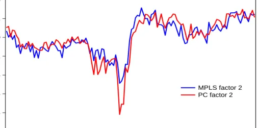
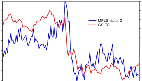
PC are plotted in Figure 3. Once again, they are similar but differ in detail, especially around the crisis. One possible interpretation is that the indices capture monetary conditions - gradu-ally tightening pre-crisis, then loosening as rates fall and the exchange rate depreciates, followed thereafter by a gradual tightening as the real exchange rate unwinds. It is also interesting that the (inverted) second factors move in a similar manner to the Goldman-Sachs FCI (Figure 4). We tentatively interpret the second factor and GS ‘FCI’ as monetary conditions indices.
6
Forecast performance
It is of obvious interest to have timely updates of forecasts, and forecast performance is a useful performance metric. So in this section we recursively estimate the FCIs and forecasting models, and then forecast monthly GDP growth using an AR(2) augmented with our FCIs. The NIESR series. We use this because it is a timely series (available with a short lag) at a policy-useful frequency (monthly), and also an object of considerable policy interest (being essentially interpolated GDP). It is well established (e.g. Groen et al. (2009)) that good benchmarks for GDP forecasts include low order AR processes, so our benchmark is a simple AR(2). We also
wish to examine the role of different sets of target variables (they), the six private-sector spreads
and the complete set of 28 financial indicators.
-10 -8 -6 -4 -2 0 2 4 2004 2005 2006 2007 2008 2009 2010 2011 2012 2013 2014 MPLS factor 2 PC factor 2
MPLS factor 2 FCI and PC factor 2 indicate the second MPLS and PC factors respectively.
Figure 3: UK MPLS and PC second factors
observations for h = 1) at forecast horizons h = 1 to 12 months. The data are quasi-real-time,
meaning that they take no account of revisions but do include the ‘ragged edge’. This does not affect the FCI-GS, as it uses exclusively financial data which are very timely. The tables below show relative root mean square forecast errors (RRMSE) from models using throughout two own-lags and two FCI lags for each of the candidate indices. A value less than 1 indicates better relative performance. In all cases we tested for better performance against the benchmark (and for the benchmark against the model in question) using Diebold Mariano (DM) tests.
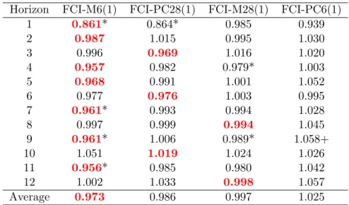
Table 2 shows that the M6 and PC28 are the two best performers, with the FCI-M6 having the best average performance and in 7 out of 12 cases the best performance at any horizon. In four cases the FCI-M6 is significantly better than the benchmark, compared to only one for the FCI-PC28. While FCI-M6 is overall best the FCI-PC28 is not dramatically worse and in some cases better, so we tested each model against the other with A DM test. In no cases were the improvements significant. FCI-M6 is particularly good at the shortest horizon (1 month) with a significant reduction in RMSE of 13.9%, which practically is very important. For MPLS, if the number of target MPLS variables is increased (FCI-M28) then performance deteriorates markedly, while if the PC uses the smaller set of indicators MPC (FCI-PC6) performance falls still more dramatically in most cases, and in one case is significantly worse than the benchmark.
The relative performance of small and large y differ between the two methods. With MPLS
performance falls off when the target indicators are increased. Specifically, in 9 out of 12 cases performance worsens, in two cases significantly (results not reported in the table), on average by 1.26%, and at horizon 1 by a significant and substantial 14.3%. By contrast, increasing the PC
-3 -2 -1 0 1 2 3 4 93 94 95 96 97 98 99 100 101 102 04 05 06 07 08 09 10 11 12 13 14 MPLS factor 2 GS FCI
MPLS factor 2 and GS FCI indicate the (inverted) second MPLS factor and the Goldman-Sachs FCI respectively.
Figure 4: UK MPLS second factor and Goldman Sachs financial conditions index
set from 6 to 28 invariably increases performance, on average by 3.8% and significantly so in half the cases (results not reported in the table). Thus we conclude that while the conventional PC approach is useful, the targeted MPLS method using a small number of spreads almost always dominates, and that in the MPLS using the large target set worsens performance.
6.1 More factors
Next we consider whether using more factors improves performance.
Table 3 reports the results of using the first two factors (indicated in the table by, eg, FCI-M6(2) where “(2)” indicates the number of included factors). On average, there is an improvement in performance in each case. The FCI-M28(2) is now on average the best, although at the policy-important first horizon the FCI-M6(2) is ahead by a large margin, with a dramatic and significant RMSE improvement over the benchmark of 20.3%. Moreover, this performance is significantly better than that of the FCI-PC28(2). No other comparisons between the two are significant. Arguably the small FCI-M6(2) results are better than those from the FCI-M28(2), being significantly better than the benchmark in 3 cases, best in half the cases (one more that the for M28) and with the large advantage at the one-month ahead horizon. The PC results are a small improvement over one factor but in almost all cases remain worse than the one-factor MPLS results.
Table 4 shows that adding a further factor marginally worsens average performance in all but the FCI-M28(3), which is marginally improved and is again on average best. Although the
Horizon FCI-M6(1) FCI-PC28(1) FCI-M28(1) FCI-PC6(1) 1 0.861* 0.864* 0.985 0.939 2 0.987 1.015 0.995 1.030 3 0.996 0.969 1.016 1.020 4 0.957 0.982 0.979* 1.003 5 0.968 0.991 1.001 1.052 6 0.977 0.976 1.003 0.995 7 0.961* 0.993 0.994 1.028 8 0.997 0.999 0.994 1.045 9 0.961* 1.006 0.989* 1.058+ 10 1.051 1.019 1.024 1.026 11 0.956* 0.985 0.980 1.042 12 1.002 1.033 0.998 1.057 Average 0.973 0.986 0.997 1.025
The table reports relative root mean square error (RRMSE) of an AR(2) augmented with two lags of the first factor from the indicated FCI relative to an AR(2). The best performer in any row is indicated by bold. * records that a DM test indicates the model is significantly better than the AR at 5%. + records that a DM test indicates the AR is significantly better than the model at 5%.
Table 2: Forecast performance monthly GDP, FCI (first factor) relative to AR(2)
performance of the narrow FCI-M6(3) narrowly deteriorates, there is an interesting pattern. At low horizons (1, 2 and 3) they are the best forecasts, there is a further improvement in all horizons up to 6 and the performance at horizon 1 relative to the benchmark is a remarkable 25.0%, which once again is significantly better than for FCI-PC28(3). Again, no other comparisons between the two are significant. At higher horizons performance for FCI-M6(3) generally deteriorates relative to FCI-M6(2), while the large FCI-M28(3) is best at horizons 4 to 9. With the principal component methods, overall and in the majority of cases performance is worse
The conclusion is that the small-yMPLS based FCI-M6 is a candidate for the best performer
and that while using one factor is very effective, using further factors is useful, especially at low horizons. Had we restricted attention to the one-month ahead forecasts, the FCI-M6 would have been unambiguously selected, and by a very large margin. At medium horizons the FCI-M28(3) is a strong contender. The principal components FCI-PC28 also has forecasting power, but less so than for the MPLS variants and with only the first or second factors.
6.2 Instabilities and lagged y
So using the full available sample for estimation, the FCI-M6 tends to outperform the alternatives
we consider in a recursive exercise. But it is possible that there are instabilities in either
Horizon FCI-M6(2) FCI-PC28(2) FCI-M28(2) FCI-PC6(2) 1 0.797* 0.859 0.832* 0.947 2 0.988 1.019 0.959 1.020 3 0.971 0.973 0.952 1.012 4 0.953 0.985 0.921 0.980 5 0.961 0.992 0.952 1.037 6 0.951 0.971 0.955 0.974 7 0.946 0.987 0.961 0.985 8 0.985 0.996 0.947 1.010 9 0.951* 1.006 0.992 1.012 10 1.066 1.008 1.023 0.968 11 0.932* 0.973 0.974 0.983 12 0.990 1.028 0.996 1.012 Average 0.958 0.983 0.955 0.995
The table reports relative root mean square error (RRMSE) of an AR(2) augmented with two lags of the first two factors from the indicated FCI relative to an AR(2). The best performer in any row is indicated by bold. * records that a DM test indicates the model is significantly better than the AR at 5%. + records that a DM test indicates the AR is significantly better than the model at 5%.
Table 3: Forecast performance monthly GDP, FCI (first two factors) relative to AR(2)
Horizon FCI-M6(3) FCI-PC28(3) FCI-M28(3) FCI-PC6(3)
1 0.750* 0.847* 0.836* 0.963 2 0.974 1.015 0.989 1.016 3 0.949 0.972 0.961 1.026 4 0.930 0.985 0.917 0.982 5 0.953 0.998 0.940 1.051 6 0.951 0.980 0.940 0.978 7 0.957 0.995 0.947 0.997 8 0.970 1.019 0.933 1.009 9 1.003 1.022 0.983* 1.017 10 1.066 1.027 1.023 0.964 11 0.958* 0.984 0.969 0.978 12 1.043+ 1.053+ 0.997 1.002 Average 0.959 0.991 0.953 0.999
The table reports relative root mean square error (RRMSE) of an AR(2) augmented with two lags of the first three factors from the indicated FCI relative to an AR(2). The best performer in any row is indicated by bold. * records that a DM test indicates the model is significantly better than the AR at 5%. + records that a DM test indicates the AR is significantly better than the model at 5%.
Horizon 1 0.852* 2 0.993 3 0.990 4 0.960 5 0.960 6 0.982 7 0.962 8 0.987 9 0.955* 10 1.052 11 0.954 12 0.992 Average 0.970
The table reports relative root mean square error (RRMSE) of an AR augmented with two lags of the first factor from the FCI-M6 relative to an AR(2) augmented with two lags of the Goldman Sachs FCI (AR+GS). * records that a DM test indicates the model is significantly better than AR+GS at 5%. Evaluation period 2011M06 to 2014M06.
Table 5: Forecast performance monthly GDP, FCI-M6 (first factor) relative to FCI-GS
(2013) conclude that full-sample estimation of principal components is remarkably robust to the presence of structural change in the loadings, borne out in both the factor estimation and forecasting dimensions in their empirical investigation in Stock and Watson (2009). Forecasting where there are instabilities was recently surveyed by Rossi (2013). Here a robust strategy is to discount the past in some way, and one simple way to do this is with a rolling estimation window. An obvious issue is how to choose window length. Giraitis et al. (2013a) develop an optimal method for determining this, but the model considered here is too complex for that to be applied. Instead we examine estimation window lengths of 36, 48 and 60 months (compared to the recursive estimation window whose starting sample is 90 months and then extends). Clearly, in the light of the discussion above, there is a tension between allowing forecast model instability and estimation of the factors.
For brevity we restrict attention to the MPLS based FCI with small-y which we have
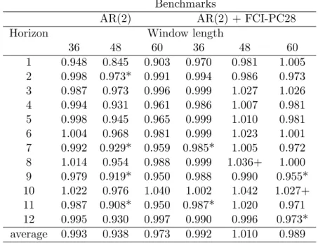
estab-lished is a good and robust performer. The results are summarised in Table 6. It emerges that for shorter windows, the FCI-M6 continues on average to beat the AR, and in some cases (win-dow 48) significantly. Similarly, for win(win-dow length 36 and 60 the FCI-M6 beats the FCI-PC28.
This is not true for a 48 period window where in one case (h=8) the FCI-PC28 is significantly
better, but overall the results lean towards support for the MPLS.
Given the emphasis in this section on forecasting, we examined the use of lagged (1 through
4) financial variables yand the contemporaneous macro data setx, speculating that this would
Benchmarks
AR(2) AR(2) + FCI-PC28
Horizon Window length
36 48 60 36 48 60 1 0.948 0.845 0.903 0.970 0.981 1.005 2 0.998 0.973* 0.991 0.994 0.986 0.973 3 0.987 0.973 0.996 0.999 1.027 1.026 4 0.994 0.931 0.961 0.986 1.007 0.981 5 0.998 0.945 0.965 0.999 1.010 0.981 6 1.004 0.968 0.981 0.999 1.023 1.001 7 0.992 0.929* 0.959 0.985* 1.005 0.972 8 1.014 0.954 0.988 0.999 1.036+ 1.000 9 0.979 0.919* 0.950 0.988 0.990 0.955* 10 1.022 0.976 1.040 1.002 1.042 1.027+ 11 0.987 0.908* 0.950 0.987* 1.020 0.971 12 0.995 0.930 0.997 0.990 0.996 0.973* average 0.993 0.938 0.973 0.992 1.010 0.989
The table reports relative root mean square error (RRMSE) of an AR(2) augmented with two lags of the first factor of the FCI-M6 relative to benchmarks. * records that a DM test indicates the model is significantly better than the benchmark at 5%. + records that a DM test indicates the benchmark is significantly better than the model at 5%. Evaluation period 2011M06 to 2014M06.
Table 6: Relative forecast performance of an AR(2) with FCI-M6(1) relative to an AR(2) and AR(2) with FCI-PC28 over varying estimation windows
macro variables). There is a cost to this as we lose effective observations. In the event, forecast
performance is little changed. For a lead of 1, there is an improvement ath= 1 against the AR
benchmark but on average no improvement and no change relative to the PC augmented AR.
For a lead of 4, there is a more marked improvement ath = 1 against the benchmarks, and on
average a small improvement. But there is little forecast advantage gained and it weakens the interpretation as a factor informative about contemporaneous financial shocks, so in the rest of this paper we continue to use that reported above.
7
Identifying credit supply shocks
We have interpreted our FCI in a quasi-structural sense, but it is also possible to identify credit supply shocks in a genuinely structural sense with identifying restrictions in an SVAR. In this section we therefore use sign restrictions to back out such structural shocks from a small VAR, and ask whether the first factor from FCI-M6, which has the clearest interpretation as an FCI, can help with this identification. We also experimented with additional factors but were unable to identify the SVAR when we did so.
We begin with a VAR including CPI inflation (untransformed), growth (NIESR monthly GDP estimates), loans (PNFC lending, log differenced), bank lending spreads on loans to PNFCs (untransformed) and LIBOR (differenced), which we then augment with the FCI (differenced) from the FCI. The data are shown in Chart 5.
We have 126 monthly observations. We then identify monetary policy and credit supply shocks using the scheme used in Paries et al. (2014) (following e.g. Busch et al. (2010), Gambetti and Musso (2012) and Peersman (2012)).
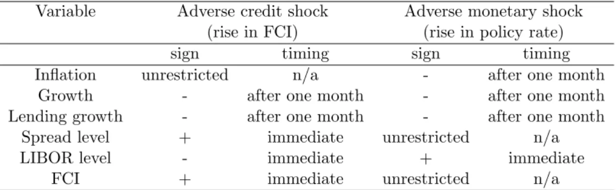
Specifically, a positively-signed monetary policy shock, i.e. an unexpected increase in the short-term interest rate, depresses activity, prices and loans. A positively-signed credit supply shock associated with a softening of the financing environment raises activity and tightens the policy rate. The impact on prices is left unrestricted as the positive effect on demand can be mitigated by a positive effect on supply. Both a positive monetary policy shock and a negative credit supply shock depress loans and activity. In order to dissociate a positive credit supply shock from an expansionary monetary policy shock, we impose a different sign on the monetary policy rates and impose a fall in the bank lending spread after a positive credit supply shock. In the augmented VAR a negative credit supply shock raises the FCI. We examine one-month responses and following Paries et al. (2014) for the non-financial series (activity, prices and loans) we impose the sign restrictions starting one month after the shock. All this is summarised in Table 7.
We estimate the impulses using the method employed in Giraitis et al. (2013b).
Figure 6 and 7 show impulse responses following a 1 standard deviation shock up to 40 months for all variables in the SVARs, each estimated with six lags. Figure 6 reports the impulses from
Variable Adverse credit shock Adverse monetary shock
(rise in FCI) (rise in policy rate)
sign timing sign timing
Inflation unrestricted n/a - after one month
Growth - after one month - after one month
Lending growth - after one month - after one month
Spread level + immediate unrestricted n/a
LIBOR level - immediate + immediate
FCI + immediate unrestricted n/a
Table 7: Sign and timing restrictions
an SVAR(5) including inflation, growth, lending growth, spread level and LIBOR level by row, where the first column reports the response to an adverse monetary shock (tightening, higher rates) and the second an adverse credit shock (tightening, associated with higher FCI) together with 90% confidence bounds generated by bootstrapping the reduced form VAR, its coefficients
and reduced form IRFs and using the A(0) matrices obtained by sign restrictions to take the
median of the bootstrapped structural IRFs. Figure 7 repeats the exercise for SVAR(6), with the addition of the FCI-M6.
Our sample is short, and for more than half of the period we are at the effective lower bound, where for obvious reasons it may be hard to identify monetary shocks. The Bank of England uses a ‘shadow’ interest rate for internal purposes, which takes account of the estimated effect of asset purchases (quantitative easing) and may therefore be negative. But using this in place of LIBOR did not substantially change results. Nevertheless, in most cases they are easily interpretable.
Looking first at the effect of a monetary shock, in the SVAR(5) excluding FCI a monetary shock has a moderately persistent negative impact on inflation which temporarily overshoots by a small amount in the recovery before returning to a persistent negative impact. A strict impact price puzzle is ruled out by assumption, but the negative impact is sustained for roughly nine periods. There is a perverse unconstrained impact effect on output growth, and after the negative restriction kicks in the impulse oscillates around the asymptote, which is less intuitive. Lending contracts briefly. The unrestricted impact on spreads is negative and very persistent. LIBOR reacts positively and the impact decays rapidly and non-monotonically, with a somewhat counter-intuitive trough at 3 months. Including FCI, the inflation profile in the two SVAR(6)s are extremely similar to that in the SVAR(5). The output effect is similar, as is lending growth. The effects on spreads, however, are quite different, initially positive then persistently negative. The effect on LIBOR is broadly similar. Following a negative impact the FCI oscillates between positive and negative values.
SVAR(6) but is much larger (and smoother) in the latter case with a small positive impact at long horizons. The implication is that credit shocks have a larger impact on output supply than demand. This raises the question of whether the identified shock is in fact conflating a credit and supply (productivity) shock. Helbling et al. (2011), who identify a credit and productivity shock in a related exercise, argue that it is important to impose a non-negativity (given a positive credit shock) impact on productivity from a credit shock. But we find this hard to justify, given that a part of the impact of credit shocks is likely to be on supply, perhaps via working capital entering the production function as in Fernandez-Corugedo et al. (2011), or research and development expenditure affecting TFP as in Millard and Nicolae (2014). Obvious sign restrictions that would help identify a supply shock are that following an adverse supply shock growth falls and inflation rises, but no other restrictions are evident in our framework. We also note below that our identified credit shock has a large and significant impact in the SVAR(6) case which is hard to understand if the shock were to supply. For the SVAR(5) the impulse response for growth is counter-intuitively initially positive and then oscillating around the asymptote and very small. By contrast, in the SVAR(6) while effects remain small there is initially a negative impact, in accordance with our expectations, before moving to a persistent small positive impact. Lending, where we might expect a clear negative effect, after the initial impact constrained to be negative oscillates around the asymptote in the SVAR(5) cases. In the SVAR(6) after a counter-intuitive positive spike at 3 months the effect lending is persistently reduced and overall is negative, much more in line with what we expect. Spreads are restricted to initially increase, and in the SVAR(5) they then decline and become negative. By contrast, in the SVAR(6) they are uniformly positive, large relative to the effects in the SVAR(5) and very persistent, which is a more intuitive result. The impacts on LIBOR are similar in the two SVARs. The FCI itself oscillates between positive and negative values briefly (SVAR(6) only).
So the addition of our FCI to the SVAR(5) leaves many of the impulses unchanged, but materially and qualitatively affects the estimated effect of a monetary shock on spreads. The positive impact of a credit shock on inflation is much larger and without the counterintuitive impact on growth, although effects remain small. The negative persistent effect on lending is much more intuitive, as is the large uplift in spreads.
1 2 3 4 5 6 04 05 06 07 08 09 10 11 12 13 14 CPI inflation 1 2 3 4 5 6 04 05 06 07 08 09 10 11 12 13 14 -92 96 100 104 108 04 05 06 07 08 09 10 11 12 13 14 Monthly GDP -.015 -.010 -.005 .000 .005 .010 .015 04 05 06 07 08 09 10 11 12 13 14 growth 1,200,000 1,600,000 2,000,000 2,400,000 2,800,000 04 05 06 07 08 09 10 11 12 13 14 PNFC lending -.03 -.02 -.01 .00 .01 .02 .03 04 05 06 07 08 09 10 11 12 13 14 growth 0.0 0.5 1.0 1.5 2.0 2.5 04 05 06 07 08 09 10 11 12 13 14 Corporate spread 0.0 0.5 1.0 1.5 2.0 2.5 04 05 06 07 08 09 10 11 12 13 14 -0 2 4 6 8 04 05 06 07 08 09 10 11 12 13 14 Libor -2.0 -1.6 -1.2 -0.8 -0.4 0.0 0.4 0.8 04 05 06 07 08 09 10 11 12 13 14 diffrence -2 -1 0 1 2 3 4 04 05 06 07 08 09 10 11 12 13 14 FCI (MPLS) -1.5 -1.0 -0.5 0.0 0.5 1.0 1.5 2.0 04 05 06 07 08 09 10 11 12 13 14 difference
Monetary Shock Credit Shock ‐0.3 ‐0.25 ‐0.2 ‐0.15 ‐0.1 ‐0.05 0 0.05 0.1 0.15 0.2 1 3 5 7 9 11 13 15 17 19 21 23 25 27 29 31 33 35 37 39 Inflation ‐0.0015 ‐0.001 ‐0.0005 0 0.0005 0.001 0.0015 0.002 1 3 5 7 9 11 13 15 17 19 21 23 25 27 29 31 33 35 37 39 Growth ‐0.0025 ‐0.0015 ‐0.0005 0.0005 0.0015 0.0025 1 3 5 7 9 11 13 15 17 19 21 23 25 27 29 31 33 35 37 39 Lending ‐0.1 ‐0.08 ‐0.06 ‐0.04 ‐0.02 0 0.02 0.04 0.06 1 3 5 7 9 11 13 15 17 19 21 23 25 27 29 31 33 35 37 39 Spreads ‐0.06 ‐0.04 ‐0.02 0 0.02 0.04 0.06 0.08 1 3 5 7 9 11 13 15 17 19 21 23 25 27 29 31 33 35 37 39 Rates ‐0.15 ‐0.1 ‐0.05 0 0.05 0.1 0.15 0.2 0.25 0.3 1 3 5 7 9 11 13 15 17 19 21 23 25 27 29 31 33 35 37 39 Inflation ‐0.0015 ‐0.001 ‐0.0005 0 0.0005 0.001 0.0015 0.002 0.0025 1 3 5 7 9 11 13 15 17 19 21 23 25 27 29 31 33 35 37 39 Growth ‐0.004 ‐0.003 ‐0.002 ‐0.001 0 0.001 0.002 1 3 5 7 9 11 13 15 17 19 21 23 25 27 29 31 33 35 37 39 Lending ‐0.06 ‐0.04 ‐0.02 0 0.02 0.04 0.06 0.08 0.1 0.12 1 3 5 7 9 11 13 15 17 19 21 23 25 27 29 31 33 35 37 39 Spreads ‐0.08 ‐0.06 ‐0.04 ‐0.02 0 0.02 0.04 0.06 0.08 1 3 5 7 9 11 13 15 17 19 21 23 25 27 29 31 33 35 37 39 Rates
Figure 6: Impulse responses and 90% confidence bounds following adverse monetary and credit 1 SD shocks, excluding FCI.
Monetary Shock Credit Shock ‐0.3 ‐0.25 ‐0.2 ‐0.15 ‐0.1 ‐0.05 0 0.05 0.1 0.15 0.2 1 3 5 7 9 11 13 15 17 19 21 23 25 27 29 31 33 35 37 39 Inflation ‐0.0015 ‐0.001 ‐0.0005 0 0.0005 0.001 0.0015 0.002 1 3 5 7 9 11 13 15 17 19 21 23 25 27 29 31 33 35 37 39 Growth ‐0.0025 ‐0.0015 ‐0.0005 0.0005 0.0015 0.0025 1 3 5 7 9 11 13 15 17 19 21 23 25 27 29 31 33 35 37 39 Lending ‐0.1 ‐0.08 ‐0.06 ‐0.04 ‐0.02 0 0.02 0.04 0.06 1 3 5 7 9 11 13 15 17 19 21 23 25 27 29 31 33 35 37 39 Spreads ‐0.06 ‐0.04 ‐0.02 0 0.02 0.04 0.06 0.08 1 3 5 7 9 11 13 15 17 19 21 23 25 27 29 31 33 35 37 39 Rates ‐0.25 ‐0.2 ‐0.15 ‐0.1 ‐0.05 0 0.05 0.1 0.15 0.2 0.25 1 3 5 7 9 11 13 15 17 19 21 23 25 27 29 31 33 35 37 39 FCI ‐0.15 ‐0.1 ‐0.05 0 0.05 0.1 0.15 0.2 0.25 0.3 1 3 5 7 9 11 13 15 17 19 21 23 25 27 29 31 33 35 37 39 Inflation ‐0.0015 ‐0.001 ‐0.0005 0 0.0005 0.001 0.0015 0.002 0.0025 1 3 5 7 9 11 13 15 17 19 21 23 25 27 29 31 33 35 37 39 Growth ‐0.004 ‐0.003 ‐0.002 ‐0.001 0 0.001 0.002 1 3 5 7 9 11 13 15 17 19 21 23 25 27 29 31 33 35 37 39 Lending ‐0.06 ‐0.04 ‐0.02 0 0.02 0.04 0.06 0.08 0.1 0.12 1 3 5 7 9 11 13 15 17 19 21 23 25 27 29 31 33 35 37 39 Spreads ‐0.08 ‐0.06 ‐0.04 ‐0.02 0 0.02 0.04 0.06 0.08 1 3 5 7 9 11 13 15 17 19 21 23 25 27 29 31 33 35 37 39 Rates ‐0.25 ‐0.2 ‐0.15 ‐0.1 ‐0.05 0 0.05 0.1 0.15 0.2 0.25 1 3 5 7 9 11 13 15 17 19 21 23 25 27 29 31 33 35 37 39 FCI 23
8
Conclusion
Financial Conditions Indices are popular devices for summarising the state of financial (credit) markets, and for forecasting in real time. In principle, although not always in practice, they differ from the related monetary conditions indices by being composed of real variables (e.g. spreads, rather than e.g. the levels of interest rates). Yet there is no consensus about how best to create them. In this paper we draw lessons from the macroeconomic and data-rich forecasting literature, which emphasises that there are likely to be a small number of common shocks or factors driving all sectors of the economy. So instead of combining (for example by principal components) variables described as ‘financial’ and calling the resulting index an FCI, we use the information in a large set of macroeconomic variables via MPLS to create a financial factor,
which thus has a quasi-structural interpretation. Our new alternative specifically combines
a large number of macroeconomic variables weighted by the joint covariance with subsets of financial indicators. Thus unlike standard FCIs which weight specific financial variables together by some means, our approach aims to weight latent factors from the macroeconomic data set using information from financial variables.
We compare this with the more common approach using a principal component of a medium sized set of relevant financial (and, following the literature, some monetary) indicators. Despite the contrasting methodology, our new FCI yields impressions of financial market tightness which are similar but differ in detail to those generated by the more standard principal components method. Both the standard and MPLS methods are useful for forecasting monthly GDP in a quasi-real-time recursive evaluation performed over three years to 2014, but the MPLS FCIs are superior to those based on the PC on average, and significantly so in more cases than the PC versions are superior to the MPLS. Using only the first factor, the MPLS-based FCI-M6 emphasising private sector spreads is the best overall performer in a forecast race, and is particularly good at low forecast horizons, and outstandingly good for one month ahead. The second and third factors, which are less easily interpretable and which consequently we do not describe as FCIs, also improve forecast performance in the MPLS cases. The performance advantage of the (first factor) MPLS FCI over the PC version is largely maintained using different rolling windows, rather than a full available sample recursive analysis.
We also use the new FCI to identify credit supply shocks in an SVAR, where the main effects relative to one excluding FCI are to increase the positive impact of a credit shock on inflation, make lending more negative and spreads much higher.
Thus it seems that our new FCI does contain useful information about the current financial state and that the MPLS method of extracting factors from a large macro data set focussing on financial variables is useful for forecasting output growth.
Finally, we note some avenues that could be explored in future research. One would be map
FCI, possibly using the weights from rolling windows reported in Table 6. This goes somewhat against the spirit of the idea that all macroeconomic data are driven by a small set of shocks, but might give users such as policymakers more insight into the mechanics of the FCI. The
other is to do with estimation. The PC method estimates 406 ((282−28)/2) parameters while
the PLS is somewhat more parsimonious (5 weights in the y and then 82 weights on the x).
But as discussed in Chun and Keles (2010) a sparse methodology offers a solution to a large parameter space. We note that extending such methods to our case would be a major exercise and therefore defer it to another paper.
A
Appendix: macroeconomic data
Short rate
Monthly average rate of discount, 3 month Treasury bills, Sterling
CPI indices
CPI All Items Index: Estimated pre-97 2005=100
CPI INDEX 01 : FOOD AND NON-ALCOHOLIC BEVERAGES
CPI INDEX 02 : ALCOHOLIC BEVERAGES,TOBACCO & NARCOTICS CPI INDEX 03 : CLOTHING AND FOOTWEAR
CPI INDEX 04 : HOUSING, WATER AND FUELS
CPI INDEX 05 : FURN, HH EQUIP & ROUTINE REPAIR OF HOUSE CPI INDEX 06 : HEALTH
CPI INDEX 07 : TRANSPORT CPI INDEX 08 : COMMUNICATION
CPI INDEX 09 : RECREATION & CULTURE CPI INDEX 10 : EDUCATION
CPI INDEX 11 : HOTELS, CAFES AND RESTAURANTS CPI INDEX 12 : MISCELLANEOUS GOODS AND SERVICES
Surveys of activity and expectations
CBI MONTHLY TRENDS ENQUIRY Export order book
CBI MONTHLY TRENDS ENQUIRY Adequacy of Stocks of Finished Goods CBI MONTHLY TRENDS ENQUIRY Total order book
CBI MONTHLY TRENDS ENQUIRY Volume of output
CBI MONTHLY TRENDS ENQUIRY Average prices for domestic orders CBI DISTRIBUTIVE TRADES REPORTED MOTOR TRADERS SALES CBI DISTRIBUTIVE TRADES REPORTED MOTOR TRADERS ORDERS
CBI DISTRIBUTIVE TRADES REPORTED MOTOR TRADERS SALES FOR TIME OF YEAR CBI DISTRIBUTIVE TRADES REPORTED MOTOR TRADERS STOCKS
CBI DISTRIBUTIVE TRADES REPORTED RETAILING SALES CBI DISTRIBUTIVE TRADES REPORTED RETAILING ORDERS
CBI DISTRIBUTIVE TRADES REPORTED RETAILING SALES FOR TIME OF YEAR CBI DISTRIBUTIVE TRADES REPORTED RETAILING STOCKS
CBI DISTRIBUTIVE TRADES REPORTED WHOLESALING SALES CBI DISTRIBUTIVE TRADES REPORTED WHOLESALING ORDERS
CBI DISTRIBUTIVE TRADES REPORTED WHOLESALING SALES FOR TIME OF YEAR CBI DISTRIBUTIVE TRADES REPORTED WHOLESALING STOCKS
CIPS MANUFACTURING PURCHASING MANAGER’S INDEX- activity in manufacturing sector. CIPS MANUFACTURING (Consumer Goods Industries) TOTAL NEW ORDERS
CIPS MANUFACTURING SUPPLIER’S DELIVERY TIMES CIPS MANUFACTURING EMPLOYMENT
CIPS MANUFACTURING STOCKS OF FINISHED GOODS CIPS MANUFACTURING INPUT PRICES
CIPS MANUFACTURING
CIPS MANUFACTURING TOTAL NEW ORDERS CIPS MANUFACTURING OUTPUT
CIPS MANUFACTURING QUANTITY OF PURCHASES CIPS MANUFACTURING STOCKS OF PURCHASES
CPI: consumer price index; CBI: Confederation of British Industry; CIPS Chartered Institute of Purchasing and Supply survey
Sample 2004m01 to 2014m06; all variables transformed to stationarity
Labour market activity
Total Claimant count SA (UK) Claimant count rate - all - SA (UK) LMSB SA AWE total pay WE LMSB SA AWE total pay PRI
LFS: Econ inactive: UK: All: Aged 16+: 000s: SA: Annual = 4 quarter average LFS: In employment: UK: All: Aged 16+: 000s:SA: Annual = 4 quarter average LFS: Unemployed: UK: All: Aged 16+: 000s: SA: Annual = 4 quarter average
Surveys of confidence
Gfk/EC consumer confidence - question 8, major purchases at present
Gfk/EC consumer confidence - question 9, major purchases over next 12 months
House prices
House price index, All houses (All buyers),UK Nationwide House Price Index, All properties, UK
RICS Housing Market Survey, Prices, England and Wales, Net Balance
Indices of Production
IOP: B-E: PRODUCTION: CVMSA
IOP: B:MINING AND QUARRYING: CVMSA IOP: C:MANUFACTURING: CVMSA
IOP: SIC07 Output Index D-E: Utilities: Electricity, Gas, Water Supply, Waste Management IOP: CA:Manufacture of Food products beverages and tobacco
IOP: CB:Manufacture of textiles wearing apparel and leather products
IOP: CF:Manuf Of Basic Pharmaceutical Prods & Pharmaceutical Preparations IOP: CC:Manufacture of wood and paper products and printing
IOP: CJ:Manufacture of electrical equipment
IOP: CD:Manufacture of coke and refined petroleum product IOP: CE:Manufacture of chemicals and chemical products
IOP: CG:Manuf of rubberplastics prods & other non-metallic mineral prods IOP: CM:Other manufacturing and repair
IOP: CH:Manufacture of basic metals and metal products IOP: CK:Manufacture of machinery and equipment n.e.c.
IOP: CI:Manufacturing of computer electronic & optical products IOP: CL:Manufacture of transport equipment
Retail sales
RSI:Volume Seasonally Adjusted:All Retailers inc fuel:All Business Index RSI:Predominantly food stores (vol sa):All Business Index
RSI:Non-specialised stores (vol sa):All Business Index RSI:Other non-food stores (vol sa):All Business Index RSI:textiles:clothing:footwear (vol sa):All Business Index RSI:Household goods stores (vol sa):All Business Index
RSI:Volume Seasonally Adjusted:Non-store Retailing:All Business Index RSI:Value Seasonally Adjusted:All Retailers inc fuel:All Business Index OS visits to UK : Earnings
UK visits abroad: Expenditure abroad
IOP index of industrial production; RSI retail sales index
Sample 2004m01 to 2014m06; all variables transformed to stationarity
Acknowledgements
References
Andr´es, J., D. J. L´opez-Salido, and E. Nelson (2004): “Tobin’s imperfect substitution
in optimising general equilibrium,” Journal of Money, Credit and Banking, 36, 665–90.
Angelopoulou, E., H. Balfoussia, and H. Gibson(2013): “Building a financial conditions
index for the euro area and selected euro area countries: what does it tell us about the crisis?”
ECB WP no. 1541.
Bai, J. and S. Ng(2002): “Determining the number of factors in approximate factor models,”
Econometrica, 70, 191–221.
Barnett, A. and R. Thomas(2013): “Has weak lending and activity in the United Kingdom
been driven by credit supply shocks?” Bank of England Working Paper No. 482.
Bates, B. J., M. Plagborg-Møller, J. H. Stock, and M. W. Watson (2013):
“Con-sistent factor estimation in dynamic factor models with structural instability,” Journal of
Econometrics, 177, 289 – 304.
Busch, U., M. Scharnagl, and J. Scheithauer(2010): “Loan supply in Germany during
the financial crisis,” Discussion Paper Series 1: Economic Studies 2010:05, Deutsche
Bun-desbank.
Chun, H. and S. Keles (2010): “Sparse partial least squares regression for simultaneous
dimension reduction and variable selection,” Journal of the Royal Statistical Society B, 72,
3–25.
Curdia, V. and M. Woodford(2011): “The central-bank balance sheet as an instrument of
monetary policy,” Journal of Monetary Economics, 58.
de Jong, S. (1993): “SIMPLS: an alternative approach to partial least squares regression,”
Chemometrics and Intelligent Laboratory Systems, 18, 251–63.
Ericsson, N., E. Jansen, N. Kerbeshian, and R. Nymoen(1998): “Interpreting a
mone-tary conditions index in economic policy,” inTopics in Monetary Policy Modelling, Conference
Papers Vol. 6, Bank for International Settlements.
Fernandez-Corugedo, E., M. McMahon, S. Millard, and L. Rachel (2011):
“Un-derstanding the macroeconomic effects of working capital in the United Kingdom,” Bank of
England Working Paper.
Gambetti, L. and A. Musso (2012): “Loan supply shocks and the business cycle,”Working
Gauthier, C., C. Graham, and Y. Lui (2004): “Financial conditions indexes for Canada,”
BoC WP.
Gertler, M. and N. Kiyotaki(2010): “Financial intermediation and credit policy in business
cycle analysis,” .
Gilchrist, S., V. Yankov, and E. Zakrajsek (2009): “Credit market shocks and
eco-nomic fluctuations: evidence from corporate bond and stock markets,” Journal of Monetary
Economics, 56, 471–93.
Gilchrist, S. and E. Zakrajsek (2012): “Credit spreads and business cycle fluctuations,”
American Economic Review, 102, 1692–720.
Giraitis, L., G. Kapetanios, and S. Price (2013a): “Adaptive forecasting in the presence
of recent and ongoing structural change,” Forthcoming in the Journal of Econometrics.
Giraitis, L., G. Kapetanios, and T. Yates (2013b): “Inference on multivariate stochastic
time varying coefficient models,” QMUL unpublished.
Groen, J. J., G. Kapetanios, and S. Price (2009): “A real time evaluation of Bank of
England forecasts of inflation and growth,” International Journal of Forecasting, 25, 74–80.
Groen, J. J. J. and G. Kapetanios(2013): “Model Selection Criteria for Factor-Augmented
Regressions,” Oxford Bulletin of Economics and Statistics, 75, 37–63.
Guichard, S., D. Haugh, and D. Turner(2009): “Quantifying the effect of financial
con-ditions in the euro area, Japan, United Kingdom and the United States,” OECD Economics
Working Papers No. 677.
Harrison, R. (2012): “Asset purchase policy at the effective lower bound for interest rates,”
Bank of England Working Paper.
Hatzius, J., P. Hooper, F. Mishkin, K. Schoenholtz, and M. Watson(2010):
“Finan-cial Conditions Indexes: a fresh look after the finan“Finan-cial crisis,” Working Paper.
Helbling, T., R. Huidron, M. A. Kose, and C. Otrok(2011): “Do credit shocks matter?
A global perspecive,” European Economic Review, 55, 340–53.
Helland, I. S. (1988): “On the structure of Partial Least Squares Regression,”
Communica-tions in Statistics - Simulation and Computation, 17, 581–607.
——— (1990): “Partial Least Squares Regression and statistical models,”Scandinavian Journal
of Statistics, 17, 97–114.
Millard, S. and A. Nicolae (2014): “The effect of the financial crisis on TFP growth: a
general equilibrium approach,” Bank of England Working Paper.
Mueller, P.(2009): “Credit spreads and real activity,” EFA 2008 Athens Meetings Paper.
Paries, M. D., L. Maurin, and D. Moccero(2014): “Financial conditions index and credit
supply shocks for the euro area,” ECB Working Paper Series.
Pearson, K. (1901): “On lines and planes of closest fit to systems of points in space,”
Philo-sophical Magazine, 2, 559–572.
Peersman, G.(2012): “Bank lending shocks and the euro area business cycle,” Ghent
Univer-sity WP.
Rossi, B.(2013): “Advances in Forecasting under Instability,” inHandbook of Economic
Fore-casting, ed. by G. Elliott and A. Timmermann, 1203–1324.
Stock, J. H. and M. W. Watson (2002): “Forecasting using principal components from a
large number of predictors,” Journal of the American Statistical Association, 97, 1167–1179.
——— (2009): “Forecasting in dynamic factor models subject to structural instability,” in The
Methodology and Practice of Econometrics: A Festschrift in Honour of David F. Hendry, ed. by D. F. Hendry, J. Castle, and N. Shephard, Oxford University Press, 173 – 205.
Swiston, A. (2010): “A U.S. financial conditions index: putting credit where credit is due,”
IMF WP/08/161.
Wold, H. (1982): “Soft modeling. The basic design and some extensions,” in Systems Under