A vector error correction forecasting model of the U.S. economy

WORKING PAPER SERIES

A Vector Error-Correction Forecasting Model of the U.S.

Economy.

Richard G. Anderson, Dennis Hoffman

and Robert H. Rasche

Working Paper 1998-008C

http://research.stlouisfed.org/wp/1998/1998-008.pdf

FEDERAL RESERVE BANK OF ST. LOUIS Research Division

411 Locust Street St. Louis, MO 63102

______________________________________________________________________________________ The views expressed are those of the individual authors and do not necessarily reflect official positions of the Federal Reserve Bank of St. Louis, the Federal Reserve System, or the Board of Governors.

Federal Reserve Bank of St. Louis Working Papers are preliminary materials circulated to stimulate discussion and critical comment. References in publications to Federal Reserve Bank of St. Louis Working Papers (other than an acknowledgment that the writer has had access to unpublished material) should be cleared with the author or authors.

A Vector Error-Correction Forecasting Model

of the U.S. Economy

Richard G. Anderson

Federal Reserve Bank of St. Louis

Dennis L. Hoffman

Arizona State University

Robert H. Rasche

Federal Reserve Bank of St. Louis

First version: May 1998

This version: July 2000

The authors are, respectively, vice president and economist, Federal Reserve Bank of St. Louis; professor of economics, Arizona State University and visiting scholar, Federal Reserve Bank of St. Louis; and senior vice president and director of research, Federal Reserve Bank of St. Louis.

We thank for our colleagues and Dean Croushore for helpful comments; Macroeconomic Advisers of St. Louis, Missouri, for providing their historical forecasts; and Marcela Williams for research assistance. Views expressed herein are those of the authors and do not necessarily reflect opinions of the Federal Reserve Bank of St. Louis, the Federal Reserve System, or their respective staffs.

Abstract

Any research or policy analysis in economics must be consistent with the time-series properties of observed macroeconomic data. Numerous previous studies reinforce the need to specify correctly a model’s multivariate stochastic structure. This paper discusses in detail the specification of a Vector Error Correction forecasting model that is anchored by long-run equilibrium relationships suggested by economic theory. The model includes six variables—the CPI, the GDP price index, real money balances (M1), the federal funds rate, the yield on long-term (10-year) government bonds, and real GDP—and four cointegrating vectors. Forecasts from the model for the 1990s compare favorably to alternatives, including those made by government agencies and private forecasters.

Richard G. Anderson

Federal Reserve Bank of St. Louis Research Division P.O. Box 442 St. Louis MO 63166-0442 [email protected] Dennis L. Hoffman Professor of Economics Arizona State University Tempe AZ 85281 [email protected] Robert H. Rasche

Federal Reserve Bank of St. Louis Research Division

P.O. Box 442

St. Louis MO 63166-0442 [email protected]

This is an exercise in applied macroeconomic forecasting. Its basis is a policy-oriented vector autoregressive model (VECM) that is anchored by long-run equilibrium relations suggested by economic theory. These relations are identified in, and are common to, a broad class of macroeconomic models. We examine the estimated model’s stability, and compare its out-of-sample forecast performance to simple random walk models and to forecasts made by government and professional forecasters. The results reveal that the VECM performs well relative to both.

Numerous previous studies of macroeconomic time-series data suggest a need for careful specification of the model’s multivariate stochastic structure. Following the classic work of Nelson and Plosser (1982), many studies have demonstrated that macroeconomic time series data likely include

components generated by permanent (or at least highly persistent) shocks.1 Yet, economic theory

suggests that at least some subsets of economic variables do not drift through time independently of each other: ultimately, some combination of the variables in these subsets, perhaps nonlinear, reverts to the mean of a stable stochastic process.2 Granger (1981) defined variables whose individual data generating processes are well-described as being driven by permanent shocks as integrated of order 1, or I(1), and defined those subsets of variables for which there exist combinations (linear or nonlinear) that are well-described as being driven by a data generating process subject to only transitory shocks as cointegrated.3

Many recent cointegration studies have shown that some individually I(1) variables—including real money balances, real income, inflation, and nominal interest rates—may be combined in linear relationships that are stationary, or I(0). We focus particular attention on these aspects of the model’s stochastic structure. Evidence on the stationarity of linear money demand relations has been presented by Hoffman and Rasche (1991), Johansen and Juselius (1990), Baba, Hendry, and Starr (1992), Stock and Watson (1993), Hoffman and Rasche (1996a), Crowder, Hoffman and Rasche (1999) and Lucas (1994),

1

Statistical tests to differentiate series with unit roots (permanent shocks) from ones with “near unit roots” (extremely persistent transitory shocks) are known to have very low power to discriminate the two alternatives. Hence it is impossible to be certain of the existence of permanent shocks and model specification becomes a choice problem on how best to minimize the dangers of specification error (Christiano and Eichenbaum, 1990).

2

The processs might include a time trend. For early discussions of “Great Ratios” in macroeconomics, see Klein and Kosobud (1961) and Ando and Modigliani (1963).

among others. Evidence in favor of an equation that links the income velocity of money to nominal interest rates, in several countries, is presented by Hoffman, Rasche and Tieslau (1995). Mishkin (1992), Crowder and Hoffman (1996) and Crowder, Hoffman and Rasche (1999) present evidence of a Fisher equation, and Campbell and Shiller (1987, 1988) have examined cointegration among yields on assets with different terms to maturity.4

The VECM model includes six variables—real GDP, the GDP deflator, the CPI, M1, the federal funds rate, and the constant-maturity yield on 10-year Treasury securities—and four cointegrating vectors. In our specification tests, we do not reject restrictions that when applied to these cointegrating

vectors achieve overidentification of the long-run equilibrium economic model.5 The model’s dynamics,

on which macroeconomic theories are largely silent, are unrestricted and determined by the sample data. The long-run relationships included in our model address, in a formal way, the classic problem of combining long-run “equilibrium” or balanced-growth relationships—ones in which the researcher derives a high degree of confidence from economic theory—with a short-run dynamic structure on which economic theory provides little guidance. During the 1970s, many analysts noted that the forecaster— more than the forecasting model—might be responsible for the performance of the model. Rasche (1981) equated this, in part, to researchers embedding sets of constraints or relationships in their models via judgmental adjustments following extensive simulation experiments. A clear statement of the nature of these constraints, at least for the MPS model, is offered by Ando (1981, p. 329):

"For practicing econometricians, extracting propositions from existing economic theory that are usable for specifying and identifying estimatable equations is an excruciatingly difficult task. I believe that this is partly because most of economic theory consists of comparative static propositions, while historical data are generated by a dynamic economy and do not directly bear evidence on comparative static propositions of economic theory. My own strategy in dealing with this problem has been to make sure that all equations, or system of equations, which I use as the bases for empirical studies,

3 _{Nonstationary variables can be integrated or cointegrated of different degrees. We restrict our focus here to}

variables that are integrated of order one.

4

Evidence in support of most of these cointegration relations also is compiled in experiments presented in Hoffman and Rasche (1996a).

5 _{See Hoffman and Rasche (1996a) for a discussion of the necessary and sufficient conditions to achieve}

have associated with them proper steady state solutions to which comparative static propositions do apply ..."

Rasche (1981) notes that, in principle, such restrictions should be made explicit and incorporated into a constrained FIML estimator.6 To a large extent, this goal is achieved in this analysis.7

In the next section, we discuss model specification and tests of the model’s four cointegrating vectors. In section 2, we examine the estimated parameters of the dynamic vector autoregressive portion of the model, and perform stability tests on the model. In section 3, we discuss the forecasting properties and performance of the estimated model with particular reference to the 1990 recession and the 1994 expansion, and compare the model’s performance to government and private forecasts during 1990–98. Section 4 contains our conclusions.

1. Testing for Cointegration

Our model is a reduced rank Gaussian VAR (Johansen, 1991)

t t t

d

X

Y

=

+

,

∑

=

Π

−

+

=

6 1 i i t i t t

X

X

ε

which is equivalent to

∑

= − −

+

Φ

∆

+

Γ

+

Π

=

∆

5 1 1 1 _i i t t t t t

X

X

d

X

ε

,

∑

=

Π

+

−

=

Π

6 1 6 _i i

I

or,

∑

= − −

+

Φ

∆

+

Γ

+

′

=

∆

5 1 1 1 _i i t t t t t

X

X

d

X

α

β

ε

.

Variables in the model include: the log of real GDP (gdp), equal to GDP deflated by the implicit price deflator for GDP (which equals the chained-dollar GDP measure introduced in 1996); the log of real M1 money balances (m1p), equal to nominal M1 deflated by the GDP deflator; two measures of inflation: log first differences of the GDP deflator (infdef) and of the CPI (infcpi) both expressed as percent annual rates; the constant-maturity yield on 10-year Treasury securities (lrate) and the federal funds rate (funds).

6 _{The process described by Ando also may be interpreted as a calibration exercise in which the dynamic model is}

constrained to satisfy certain long-run balanced-growth relationships. During the last decade, such calibration exercises have become a hallmark of the real business cycle–general equilibrium modeling literature.

7 _{Our VECM model is estimated via a contrained FIML procedure (Johansen’s estimators are constrained FIML}

The data span 1955 Q1 to 1998 Q4 and are from the Federal Reserve Bank of St. Louis database, FRED.8 The order of integration of these series has been widely discussed in the literature; we assume that each series either maintains a single unit root or is well approximated by an I(1) process.9 The sole

deterministic variable (other than intercepts) included is a dummy variable, D79, discussed further below. Our model, a six-dimension vector process, includes four long-run cointegrating relationships: a money demand (velocity) equation, a Fisher equation relating nominal interest rates and inflation, a term structure equation connecting the federal funds rate and long-term bond yields, and a relationship between two measures of inflation. To illustrate the cointegration space that spans the four steady-state relations in the VAR representation of our model, order the variables as

′ =

z

_t

{m1p , infdef , funds , infcpi , gdp , lrate }

_{t t t t t t}

Then the cointegration space that reflects the four hypothesized long-run relations may be written as:

              − − − − = ′ 1 0 1 0 0 0 1 0 0 1 0 0 1 0 0 0 1 0 1 0 0 0 1 β₁ β

The first row of β′ captures the money demand equation, the second and fourth rows measure the Fisher

relations using the two distinct measures of inflation in our system, and the third row captures the term structure spread linking the Federal funds rate and the long-term government rate. Note that the

representation of the cointegration space is not unique. Several alternative normalizations of β also yield long-run relations that embody our system of cointegrating relations. For example, there exists an observationally equivalent representation of β that contains only a single Fisher relation and a separate

8

Data for M1 from 1955-1958 are from Rasche (1987). The data are as-of December 1998, except for data used to calculate forecast errors in Figures 5–8 which are as-of July 1999. M1 in this study includes estimates of the amount of transaction deposits swept by banks into money market deposit accounts (MMDA), beginning in 1994. Data and background information regarding such sweep programs are available from the Federal Reserve Bank of St. Louis at <www.stls.frb.org/research/swdata.html>..

9 _{The assumption that inflation is an I(1) process is equivalent to assuming that the log of the price level is an I(2)}

relation linking the two inflation measures. Define R₁ 1 0 0 0 0 1 0 0 0 0 1 0 0 1 0 1 = −            

. Then R1β′ is the matrix of

cointegrating vectors reflecting a stationary spread between the inflation rates and a single Fisher equation

between the deflator inflation rate and the funds rate. Alternatively, define R₂

1 0 0 0 0 1 0 1 0 0 1 0 0 0 0 1 = −             .

Then, R2β′ is the matrix of cointegrating vectors reflecting a stationary spread between the inflation rates

and a single Fisher equation between the CPI inflation rate and the funds rate. Similarly interest elasticity and Fisher relations could be expressed in terms of the funds rate rather than the long-term rate. Let

R₃ 1 1 0 0 0 1 1 1 0 0 1 0 0 0 1 1 = − −             β

; then R3β′ is the matrix of cointegrating vectors reflecting the two Fisher

equations and the money demand vector in terms of the funds rate. However, the class of steady-state relations is sufficient to satisfy conditions for identification of cointegration spaces discussed in Hoffman and Rasche (1996a)

In our system of r = 4 cointegrating relations, r-1 = 3 restrictions satisfy the conditions for identification for each of the cointegrating relations. These restrictions appear with double underscore

(

0

) in the representation for β′ depicted above. The “ones” down the main diagonal of the expression

represent normalizations, but values in all remaining entries may in principal be tested in empirical analysis.

Testing Cointegration

Perhaps the most common approach to test for the number of cointegrating vectors is to apply an estimation technique such as Johansen (1991). In our model, an alternative approach is available because

the coefficients in three of the cointegrating vectors are “known” a priori, that is, the presumed stationary weighted sums are prespecified by economic theory. This information allows us to apply tests that have higher power to discriminate between stationarity and nonstationarity alternatives than do general testing procedures.

We first verify that the two real interest rates (rows 2 and 4 of β) are stationary. It is well known that standard tests for stationarity (unit roots) may yield incorrect inferences when the data generating process has shifted during the sample. Because a number of studies have found evidence that real interest rates shifted sometime after the beginning of the Federal Reserve’s “New Operating Procedure” in 1979, we augment a standard Dickey-Fuller regression with a dummy variable D79, whose value is 0.0 through 1979 Q3 and 1.0 thereafter. The “t-ratios” of –3.63 and –3.71, respectively, on the coefficients of the lagged real rates (Table 1, columns 1 and 2) support the stationarity of the short-term real interest rates; the negative coefficients on D79 support Huizinga and Mishkin’s (1986) conclusion that real rates

increased around the time of the New Operating Procedure.10 The estimated coefficients on the lagged

real rates, –0.26 and –0.24, yield normalized bias test statistics; [T*(ρ-1)], of –42.6 and –39.4. These provide strong evidence, based upon conventional critical values, against a unit root in these series. The Perron (1989) “break adjusted” critical value for the normalized bias test that corresponds to the D79 parameterization is –25.4 at the 5% level so this inference remains after accounting for the shifts in the deterministic components.

Our next test is to examine the stationarity of the term structure spread. Research by Campbell and Shiller (1987, 1988) suggests that this spread is stationary, consistent with the implications of a rational expectations hypothesis of the term structure of interest rates. The “t-ratio” on the lagged term spread in the Dickey-Fuller regression is –4.14 (Table 1, column 3) supports this conclusion.

We conducted multivariate tests to establish cointegration rank in the 6 dimension system using a model with 6 lags in the VAR specification and the dummy variable D79 to allow for shifts in the

deterministic drift of the nonstationary processes and for shifts in the equilibrium real interest rate after

the New Operating Procedures period.11 The tests are based on quarterly data from 1957 Q1—1997 Q4,

omitting 1979 Q4—1981 Q4. The later period is omitted because the semilog functional form used in this model does not have adequate curvature to approximate M1 velocity in a range of nominal interest

rates above about 10 percent (see Hoffman and Rasche, 1996a).12

Johansen tests reveal considerable support for four cointegrating vectors as hypothesized in the model. The λ-max test statistic for the test of r<=3 is 18.1, which compares with a conventional 5% critical value of 14.3 and a 5% critical value of 12.0 obtained by simulation of Johansen and Nielson’s (1993) DisCo program.13 The trace test statistic is 26.1, which compares with conventional and Johansen–Nielson crticial values of 29.7 and 24.9, respectively.

The long-run money demand relation, two Fisher relationships, and the term structure relationship embody a total of 7 over-identifying restrictions (1 in the money demand equation and 2 in each of the other 3 relations) that apply to the cointegrating space. The critical value for the test of these 7 restrictions is 14.08 at the 5% level. The value of the Chi-Squared Likelihood ratio test statistic of these restrictions is 14.12. On the margin the restrictions are not inconsistent with the data. Note that the matrix of

cointegrating vectors, β, contains both known and unknown coefficients. Johansen and Juselius (1992)

extended the standard Johansen FIML estimator to deal with this case, and we use their method to estimate the interest semielasticity of M1 velocity,βˆ1, conditional on the three “known” cointegrating

10

Recall that the distribution of estimated coefficients in Dickey-Fuller regressions depends on the form of any deterministic terms included the equation (e.g., Schmidt, 1990). Perron (1989) suggests that the 5% critical value for our specification is –3.76.

11

Hoffman and Rasche (1996a) show that there is no significant shift in the constant of the velocity cointegrating vector before and after the New Operating Procedures period. The same conclusion applies to the estimates constructed here, though we have not attempted to constrain the intercept of this cointegrating vector to the same value in the two subperiods.

12 _{Other studies have shown that a double log specification (using the log of M1 velocity and the log of nominal}

interest rates) with an interest elasticity of around 0.5 exhibits sufficient curvature to track M1 velocity over the full range of observed nominal interest rates in the post war period (see Hoffman and Rasche, 1996a). Lucas (1994), for example, plots such a double-log velocity function with an elasticity between 0.3 and 0.7 against almost a century of U.S. data with a high correlation. Unfortunately, because the double log model involves the log transformation of interest rates, it does not allow us to incorporate the complete set of cointegrating vectors considered in this study.

vectors discussed above. The estimated interest-rate semielasticity based on data from 1957 Q1 to 1997 Q4 is βˆ₁= 0.085 with a standard error of 0.005.14

In addition to the inference from the likelihood ratio tests of cointegration and tests of the overidentifying restriction, we can refine the precision of the tests by applying the Horvath and Watson (1995) tests for cointegration rank in the presence of known cointegrating vectors.15 The first test is for a cointegration rank of four based on three known and one unknown cointegrating vector. The value of the test statistic is 157.18, with critical values of 65.52, 69.40, and 77.68 at the 10, 5, and 1 percent levels, respectively. Hence, we fail to reject the hypothesis that the cointegration rank is 4. The second and third tests reveal the strength of the evidence regarding the various cointegration vectors in the system after conditioning on a particular dimension of the cointegration space. The second test is for the existence of one unknown cointegrating vector in the presence of three known cointegrating vectors. This test provides sharp inference about the existence of a money demand vector in a multivariate system

characterized by three known vectors. The value of the test statistic is 47.63, with critical values of 23.28, 25.57, and 30.13 at the 10, 5, and 1 percent levels. The third test is for the existence of three known cointegrating vectors in the presence of one unknown cointegrating vector. The value of the test statistic, 142.80 with critical values of 39.07, 42.47, and 50.08, further bolsters the case for the three vectors already revealed in the univariate analysis. We regard this as important, since we consistently have found evidence for a velocity vector in lower dimensional systems (Hoffman and Rasche, 1991; Hoffman, Rasche and Tieslau, 1995; Hoffman and Rasche, 1996a). Hence, the analysis yields considerable support for cointegration of rank 4 in the system, with substantial support from the HW tests for cointegration vectors of the form hypothesized.

Hence, the linear model used herein is best viewed as an approximation to the true M1 velocity function that is adequate for nominal rates less than 10 percent.

13

Critical values obtained via the DisCo program allow for the effect of including the deterministic variable D79.

14 _{The full sample period prior to differencing and lags begins 1955 Q2.}

2. Model Dynamics and Stability Analysis

We have examined the robustness of the estimated interest-rate semielasticity by reestimating the model recursively starting with samples that end in 1985 Q4. In each regression we have added an additional four observations until the longest sample period ends in 1997 Q4. The results of these estimations are reported in Table 2. The estimated interest-rate semielasticities range from 0.082 to 0.112. There is some tendency for the estimated coefficient to drift lower as the sample length is increased through the mid-1980s, but since the end of 1989 the estimates are remarkably stable.

While the cointegrating vectors determine the steady-state behavior of the variables in the Vector Error Correction Model, the dynamic responses of each of the variables to the underlying permanent and transitory shocks are completely determined by the sample data without any restriction. It is apparent from the F-statistics shown in Table 3 that only a few of the estimated coefficients in the VAR portion of the model are significantly different from zero. The F-statistics test the conventional VAR-model

maintained hypothesis that all of the coefficients in a particular distributed lag are equal to zero. In Table 3, the dependent variable is indicated at the top of each column and the variable in the left hand column indicates the distributed lag that is subject to the exclusion test.

First, note that in the equation for the growth rate of real GDP none of the estimated distributed lag coefficients on changes are significantly different from zero. Second, other than its own

autoregressive structure, the only significant feedback onto the federal funds rate comes from lagged growth of real GDP. There are two significant distributed lags in the equation for the long-term interest rate—its own autoregresive structure and lagged changes in the funds rate.

The structure of the lagged-change effects in the two inflation equations—for the GDP deflator and the CPI—are similar. In both, the estimated coefficients on lagged changes in the Federal funds rate are significant, but the estimated coefficients on lagged changes in both inflation rates are not. Note that the distributed lag structures of these equations differ strikingly from VAR-type estimates of “Phillips Curves”: the latter often are specified as distributed lags in changes of an inflation rate (either the GDP deflator or the CPI) and in lags of the unemployment rate (see for example Fuhrer, 1995). In both the

equations estimated here, the estimated coefficients on the lagged changes in real output are not

significant. Lagged changes in real balances and the long-term interest rate are also significant in the CPI inflation equation, though not in the GDP price inflation equation.

Finally, changes in real balances are significantly affected by lagged changes in real balances and lagged changes in both interest rates, but not by lagged changes in real output, nor by lagged changes in either inflation rate. Lagged changes in real output enter significantly only in the federal funds rate equation.

The matrix of estimated error correction coefficients is shown in Table 4. The four error correction terms are indicated by the column headings. The first column is the real balance vector (mdciv), the second is the GDP price index–real interest rate vector (defrrciv), the third is the term structure–rate spread vector (termciv), and the fourth is the CPI real rate vector (ciprrciv). The first important feature of these estimates is that none of the variables is “weakly exogenous.” In all six equations, at least one of the estimated error-correction coefficients is significantly different from zero. Changes in real balances respond significantly only to the lagged real-balance vector. Changes in GDP price-index inflation respond significantly to all but the term-structure vector. The responses to the two rate vectors are of opposite signs. Changes in the funds rate respond significantly to both the real-rate vector formed with the GDP price index and the term-structure vector. Changes in the long-term interest rate respond significantly only to the lagged GDP price index real-rate vector. Changes in CPI inflation respond significantly to the lagged values of all vectors except the real-balance vector. Real GDP growth responds significantly to all lagged vectors except the lagged GDP price index real-rate vector.

The importance of the error correction terms in Table 4 demonstrates the amount of information, relevant to near-term forecasting, that is embodied in the VECM modeling strategy’s presumption that the short-run data generating process includes pressures to adjust toward long-run equilibria.

Stability Tests

We examined the stability of the equations in our model using several conventional Chow tests that focus on the later portion of the sample.16 Table 5 contains Chow Forecast test statistics for successive intervals starting with the first quarters of 1988 through 1997. The tests fail to reveal any evidence of equation instability that might contaminate forecasts in out-sample experiments. This conclusion is unaffected by choice of out-sample period or equation investigated. Next we examine the Chow 1-step ahead forecast test based upon recursive residuals. Results appear in Figure 1. The Figure reveals the instances where the 1-step ahead prediction significantly differs from the actual value for each of the 6 variables in our model. There are several of these instances observed in the m1p, funds, and lrate equations. But virtually all of the 5% (or lower) level occurrences appear prior to 1990. Figure 2 conducts the same exercise for the 6 variables in an N-Step ahead setting where N measures the time from the date indicated in each of the panels in the Figure to the end of the sample. Again, only in the lrate equation do we observe any significant evidence of instability. And, as in the 1-Step ahead experiments, considerable evidence of stability is observed, even in the lrate equation, over the 1990’s. We conclude that the 6 equations in our model are sufficiently stable to form the foundation for our planned set of forecasting experiments.

3. Assessing Forecast Performance

Forecasting performance may be gauged in a number of different ways. Perhaps the most familiar measures are equation-by-equation root mean squared forecast error (RMSFE) or, for a system of equations, trace RMSFE. A generalized statistic that values off-diagonal covariance among forecast errors in a system of equations, GFESM, was proposed by Clements and Hendry (1993). Finally, and perhaps most relevant, model forecasts may be compared to the forecasts produced during a variety of time periods by alternative models using similar information sets.

Our analysis reveals that, using the trace RMSFE criterion, quarterly forecasts from the VECM are comparable to forecasts from naïve random walk models. However, the generalized measure GFESM,

which places weight on forecast-error covariances, suggests that forecasts from the VECM are clearly superior to those from random walk-models, especially at short-run horizons. Finally, for year-over-year forecasts (Q4 to Q4) from 1990-1998, we find that VECM forecasts are comparable to those produced by various private forecasting services and government agencies.

Generalized Forecast Error Sample Moment (GFESM) Statistics

Clements and Hendry (1993) propose predictive likelihood statistics, invariant to particular linear transformations, that are designed to capture the relative system-wide forecast performance of alternative models. Simply stated, the GFSEM condenses the relative forecast performance of a model at all

horizons into to a single overall measure of system-forecast performance. Details on the calculation of the statistic may be found in Clements and Hendry (1993, 1995) and Hoffman and Rasche (1996b).

Following Clements and Hendry, Table 6 shows the percent reduction in the GFESM statistic due to using the VECM forecasts versus the naïve random walk with-drift model. The table reveals, similar to results produced by Clements and Hendry, that the most significant improvement occurs at short forecast horizons, with reductions of 57.3 to 85.2 percent at horizons of one year or less. The gain from using the VECM forecasts falls sharply at longer horizons, to as low as 12.8% at the four-year horizon.

Root Mean Squared Forecast Error Comparison

While the GFESM is arguably a superior metric for comparing alternative system forecasts, it also is useful to compare the VECM forecasts with those produced by a naïve random walk using a

simple variable-by-variable RMSFE comparison.17 Tables 7 and 8 depict these statistics for the VECM

and a naïve random walk model. Unlike the GFESM results, no compelling case for the VECM arises from the comparison. Indeed, there are many horizons where the random walk model actually produces RMSFE comparable to, or are smaller than, the VECM model. This result is similar to that observed by Hoffman and Rasche (1996) in their comparison of VECM models against more sophisticated VAR structures. We conclude that a systems metric such as GFESM offers a case for the VECM forecasts but,

17 _{In the random walk models, the I(1) variables in the VECM system (for example, the logs of real GDP and M1,}

when judged only by RMSFE, similar forecasts for the variables in this system are suggested on average by simple random walk specifications.

Forecast Performance in Recession and Expansion: 1990–91 and 1994–95

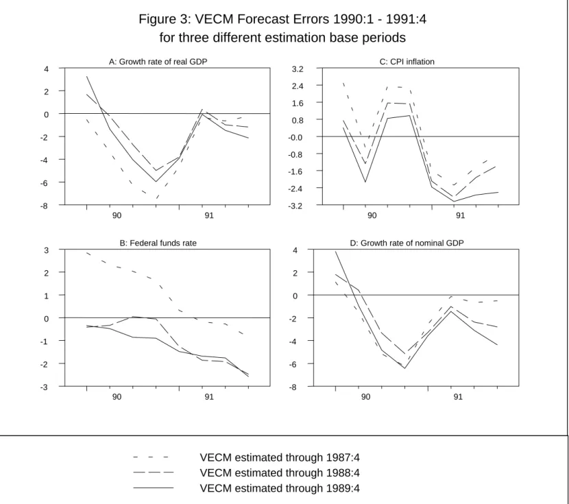
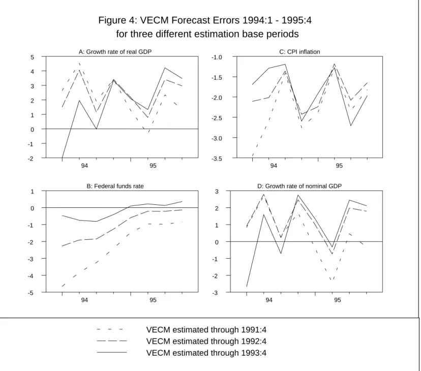
In addition to the above analysis, it is useful to analyze performance during specific subperiods. Model forecast errors for selected variables during the 1990-1991 recession period are shown in Figure 3, and during the 1994-95 expansion period in Figure 4.18 Each panel displays three sets of dynamic

forecasts errors; the dynamic forecasts begin in the first quarter following the estimation period. In Figure 3, the VECM was estimated using data samples ending in the fourth quarters of 1987, 1988 and 1989. Thus, the three forecasts shown for 1990 represent 3-year ahead (for estimation ending in 1987 Q4), 2-year ahead (for estimation ending in 1988 Q4), and 1-year ahead (for estimation ending in 1989 Q4) forecasts. Figure 4 is constructed analogously, with estimation periods ending in the fourth quarters of 1991, 1992 and 1993.

Panel A of Figure 3 reveals that, although the VECM model fails to track the sharp but brief downturn in late 1990, by the second quarter of 1991 the forecast errors for real GDP growth are modest, less than two percentage points. This pattern prevails regardless of whether the model is restricted to actual data only through the fourth quarter of 1987 (the short dashed line) or allowed access to actual data through the fourth quarter of 1989 (the solid line). Forecast errors for the federal funds rate are depicted in panel B. When allowed access to actual data through the fourth quarter of 1989, the VECM produces very accurate forecasts of the funds rate during 1990, but fails to pick up the downturn that occurred during 1991. Comparable forecast errors for the CPI inflation rate appear in Panel C. For 1990, the model performs quite well, producing forecast errors that are less than one percent on average. However, the model clearly under- forecasts the slowdown in inflation that actually occurred in 1991, resulting in forecast errors of over two percentage points for forecasts based on information through 1989. Forecast errors for the growth rate of nominal GDP are shown in Panel D. Beginning in mid-1990, nominal

growth is systematically over-predicted. From mid-1990 to mid-1991, this reflects the failure to predict the recession. After mid-1991, it reflects the failure to forecast the slowing of inflation.

The performance of the model for real GDP growth during the 1994–1995 period appears in Panel A of Figure 4. For 1994, the three and two year-ahead dynamic forecasts (that is, those with estimation periods ending in 1991 Q4 and 1992 Q4) underestimate real growth by an average of

approximately 2 percentage points. Errors for the one year-ahead forecast (estimation ending in 1993 Q4) are considerably smaller. Forecast errors for the federal funds rate over the 1994–95 period are shown in Panel B. For 1994, the three dynamic forecasts vary considerably. The one year-ahead is the most accurate, with an error averaging less than 100 basis points. The errors of the three forecasts during the second year, 1995, differ by much less. The two and three year-ahead forecasts are quite accurate, the errors averaging less than 50 basis points. Forecast errors for the CPI inflation rate appear in Panel C. The model systematically over-predicts the inflation rate for both years. The average forecast errors are around 2 percentage points. Interestingly, the amount (in percentage points) by which the model over-predicts the rate of inflation is close to the amount by which it under-over-predicts the rate of real growth. Thus, the growth rate of nominal GDP shown in Panel D is forecast quite accurately, on average, over both years and for all three dynamic forecast origins.

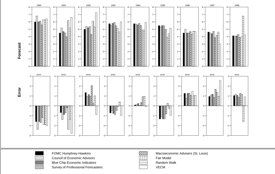
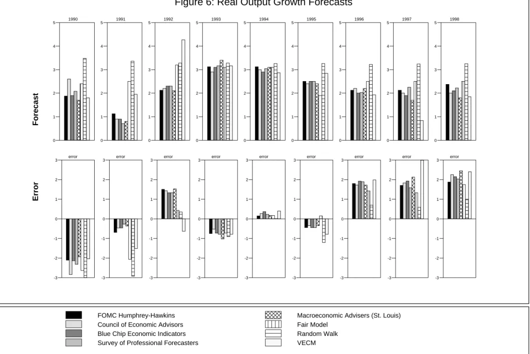
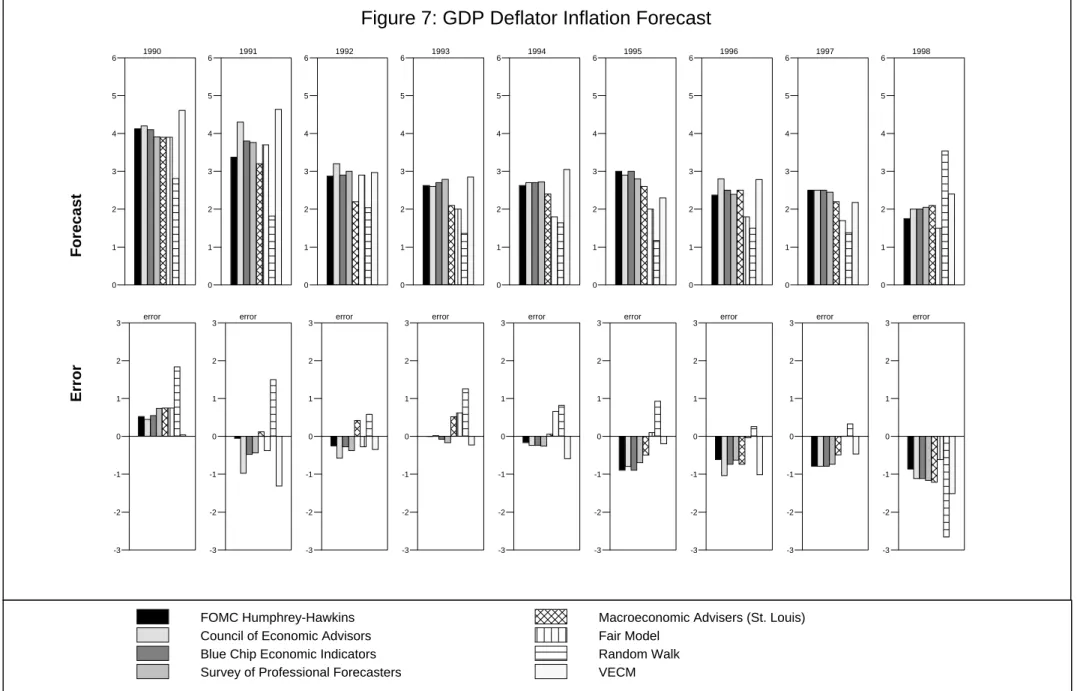
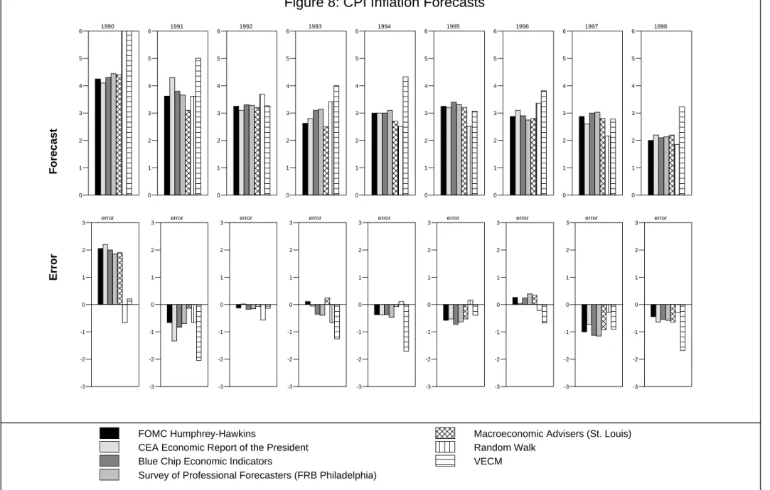
A Comparison with Alternative Forecasts: Q4–Q4

Finally, in Figures 5–8 we compare our forecasts of GDP growth and inflation on a fourth-quarter to fourth-quarter basis to seven alternatives including: federal policymakers (the midpoints of the central tendency ranges reported in the Federal Reserve’s February Humphrey-Hawkins Act testimony, and the

forecasts reported by the Council of Economic Advisers in their Annual Report);19 the consensus

forecasts reported by two surveys of private forecasters (Blue Chip Economic Indicators, and the Federal Reserve Bank of Philadelphia’s Survey of Professional Forecasters); the forecasts of the St. Louis, Missouri, consulting firm Macroeconomic Advisers; forecasts made by Ray Fair using the FAIRMODEL

at Yale University; and forecasts from univariate random-walk models. 20 The upper panels of display the forecasts, and the lower panels show the forecast error using published data available as of July 1999.

We focus on fourth-quarter to fourth-quarter forecasts made early in each year from 1990–98 (years are shown above the upper panels in the figures). The forecasts in the Humphrey-Hawkins testimony and the CEA’s Annual Report have special significance because they appear to be widely regarded as reflecting policymakers’ economic outlook for the coming year. The private sector forecasts were all prepared during late January or February, and are based on preliminary fourth quarter data. For each forecast year, the VECM and random-walk models were re-estimated with data through the previous fourth quarter so as to simulate the forecasting environment of approximately late January. Although the information sets used to prepare the forecasts likely differ somewhat, we believe they are as consistent as feasible. 21

Forecasts from the VECM system generally are comparable to the alternatives, including the random-walk model. Yet, there are some systematic differences. The VECM predicts more robust nominal GDP growth, shown in Figure 5, during the 1991–92 recovery than the alternatives and somewhat slower growth during 1997. Figures 6 and 7 provide a decomposition into forecasts of real GDP growth and inflation as measured by the price index for GDP. For the most part, forecast errors of the VECM system (the lower panels of the figures) are neither markedly better nor worse than those of the alternatives. A similar conclusion applies to forecasts of the CPI, shown in Figure 8 (the

FAIRMODEL does not forecast the CPI).

20_{Macroeconomic Advisers was previously known as Lawrence H. Meyer and Associates, and has won several}

awards for the accuracy of its forecasts; their forecasts were retrieved for us from their archives. FAIRMODEL forecasts are available on the Internet at <fairmodel.econ.yale.edu>.

21 _{Regarding the role of data revisions, we assume that forecasts of growth rates are largely invariant to revisions.}

This is the same position adopted by Fair; see <http://fairmodel.econ.yale.edu/record/index.htm>, “The Forecasting Record of the U.S. Model.” Note that while the alternative models prior to early 1996 generally were forecasting the growth of fixed-weight real GDP (and GNP) in 1987 dollars, in the figures these forecasts are compared to the growth of chain-weighted real GDP.

4. Conclusion

Our analysis of forecasting performance reveals that a VECM characterized by long-run

information in the form of Fisher equations, a term structure relationship, and a long-run money demand relation compares favorably to established alternatives, including government-agency and private-sector forecasts.

References

Ando, A. (1981), “On the Theoretical and Empirical Basis of Macroeconometric Models,” Large-Scale Macro-Econometric Models, J. Kmenta and J.B. Ramsey, eds. (North-Holland), pp. 329–58.

Ando, A. and F. Modigliani (1963), “The ‘Life-Cycle’ Hypothesis of Saving: Aggregate Implications and Tests”, American Economic Review, 53:55-84.

Baba, Y., D.F. Hendry and R.M. Starr (1992), “The Demand for M1 in the U.S.A, 1960-1988”, Review of Economic Studies, 59:25-61.

Campbell, J.Y. and R.J. Shiller (1987), “Cointegration and Tests of Present Value Models”, Journal of Political Economy, 95:1062-88.

Campbell, J.Y. and R.J. Shiller (1988), “Interpreting Cointegrated Models”, Journal of Economic Dynamics and Control, 12:505-22.

Christiano, L.J. and M. Eichenbaum (1990), “Unit Roots in Real GDP: Do We know and do We care?”, Carnegie-Rochester Conference Series on Public Policy, 32:7-61.

Christofferson, P.F. and F. X. Diebold (1996), “Cointegration and Long-Horizon Forecasting”, (mimeo) Department of Economics, University of Pennsylvania, (June).

Clements, M.P. and D.F. Hendry (1993), “On the Limitations of Comparing Mean Square Forecast Errors”, Journal of Forecasting, 617-637.

Clements, M.P. and D.F. Hendry (1995), “Forecasting in Cointegration Systems,” Journal of Applied Econometrics, 10:127-146.

Crowder, W. J. and D.L. Hoffman (1996), “The Long-Run Relationship Between Nominal Interest Rates and Inflation: The Fisher Effect Revisited”, Journal of Money, Credit and Banking, 28:102-18.

Crowder, W. J., D.L. Hoffman and R.H. Rasche (1999), “Identification, Long-Run Relations, and Fundamental Innovations in a Simple Cointegrated System”, Review of Economics and Statistics, 81:109-21.

Engle, R.F. and B.S. Yoo (1987), “Forecasting and Testing in Cointegrated Systems”, Journal of Econometrics, 35:143-159.

Fuhrer, J.C. (1995),”The Phillips Curve is Alive and Well”, New England Economic Review, 0:41-56.

Granger, C.W.J. (1981), “Some Properties of Time Series Data and their Use in Econometric Model Specification,” Journal of Econometrics 16: 121-30.

Hendry, D. F. (1995), Dynamic Econometrics (Oxford University Press)

Hoffman, D.L. and R. H. Rasche (1991), “Long-Run Income and Interest Elasticities of the Demand for M1 and the Monetary Base in the Postwar U.S. Economy”, Review of Economics and Statistics, 73:665-674.

Hoffman, D.L.and R.H. Rasche (1996a), Aggregate Money Demand Functions: Empirical Applications in Cointegrated Systems (Boston: Kluwer Academic Publishers).

Hoffman, D.L. and R. H. Rasche (1996b), “Assessing Forecast Performance in a Cointegrated System”, Journal of Applied Econometrics, 11:495-517.

Hoffman, D.L., R.H. Rasche and M. A. Tieslau (1995), “The Stability of Long-Run Money Demand in Five Industrialized Countries”, Journal of Monetary Economics, 35:317-339.

Hoffman, D.L. and S. Zhou (1997), “Testing for Cointegration in Models with Alternative Deterministic Trend Specifications: Pre-Specifying Portions of the Cointegration Space”, Department of Economics, Arizona State University, (January).

Horvath, M.T.K. and M.W.Watson (1995), “Testing for Cointegration when some Cointegrating Vectors are Known”, Econometric Theory, 11:984-1014.

Huizinga, J. and F.S. Mishkin (1986), “Monetary Policy Regime Shifts and the Unusual Behavior of Real Interest Rates”, Carnegie-Rochester Conference Series on Public Policy, 24:231-274.

Johansen, S. (1991), “Estimation and Hypothesis Testing of Cointegration Vectors in Gaussian Vector Autoregressive Models”, Econometrica, 59: 1551-1580.

Johansen, S. and K. Juselius (1990), “Maximum Likelihood Estimation and Inference on Cointegration - With Applications to the Demand for Money”, Oxford Bulletin of Economics and Statistics, 52:169-210.

Johansen, S. and K. Juselius (1992), “Testing Structural Hypotheses in a Multivariate Cointegration Analysis of the PPP and the UIP for the UK”, Journal of Econometrics, 53:211-44.

Johansen, S. and B. Nielson (1993), Manual for the simulation program DISCO.

Klein, L.R. and R. F. Kosobud (1961), “Some Econometrics of Growth: Great Ratios of Economics”, Quarterly Journal of Economics, 75:173-98.

Lucas, R.E. (1994), “On the Welfare Cost of Inflation”, (mimeo), The University of Chicago, (February).

Mishkin, F. S. (1992), “Is the Fisher Effect for Real: A Reexamination of the Relationship Between Inflation and Interest Rates”, Journal of Monetary Economics, 30:195-215.

Nelson, C. and C.I. Plosser (1982), “Trends and Random Walks in Macroeconomic Time Series:

Some Evidence and Implications,” Journal of Monetary Economics 10: 139-62.

Perron, P. (1989), “The Great Crash, the Oil Price Shock, and the Unit Root Hypothesis”, Econometrica, 57:1361-1401.

Rasche, R.H. (1981), “Comments on the Size of Macroeconomic Models,” Large-Scale Macro-Econometric Models, J. Kmenta and J.B. Ramsey, eds. (North-Holland), pp. 265–71.

Rasche, R.H. (1987), “M1 Velocity and Interest Rates: Do Stable Relationships Exist?”, Carnegie-Rochester Conference Series on Public Policy,27:9-88.

Schmidt, P. (1990). “Dickey-Fuller Tests with Drift,” Co-integration, Spurious Regressions, and Unit Roots, Thomas Fomby and George Rhodes, eds. (JAI Press, 1990), pages 161-200.

Stock, J. H. and M.W. Watson (1993), “A Simple Estimator of Cointegrating Vectors in Higher Order Integrated Systems”, Econometrica, 61:783-820.

Table 1

Dickey-Fuller Regressions 1957:1–97:4

Cointegrating vectors: defrrciv = Fisher equation using the GDP price deflator

termciv = Term structure rate spread

cpirrciv = Fisher equation using the CPI

(1) defrrciv (2) cpirrciv (3) termciv Constant -.2825 (-1.72) -.1894 (-1.16) .0943 (1.04) Xt-1 -.2631 (-3.63) -.2427 (-3.71) -.1943 (-4.14) ∆Xt-1 -.1277 (-1.41) -.2127 (-2.41) .2042 (2.57) ∆Xt-2 -.1252 (-1.43) -.2597 (-2.91) .0212 (0.26) ∆Xt-3 -.0889 (-1.07) .1066 (1.27) .0678 (0.86) ∆Xt-4 .0773 (1.00) .0353 (0.45) .0886 (1.11) D79 -.8180 (-2.59) -.7627 (-2.69) .1365 (1.05) R2 .17 .26 .08 s.e.e 1.42 1.45 0.82 Table 2

Recursive Estimates of Semielasticity of Money Demand All Samples Exclude 1979:4–81:4

Dummy Variable D79 is included

Sample Ending in: Estimated Semielasticity and Standard Error

85:4 .112(.004) 86:4 .111 (.004) 87:4 .105 (.005) 88:4 .091 (.005) 89:4 .082 (.006) 90:4 .083 (.006) 91:4 .083 (.006) 92:4 .087 (.006) 93:4 .087 (.005) 94:4 .086 (.005) 95:4 .083 (.005) 96:4 .084(.005) 97:4 .085(.005)

Table 3

F tests for Exclusion of Lagged Variables (Equations are shown in columns)

Dependent variable (equation)

∆m1p ∆infdef ∆funds ∆infcpi ∆gdp ∆lrate

∆m1p 11.93* 1.98 1.38 3.79* .58 .58 ∆infdef .37 1.37 .66 1.16 .77 .82 ∆funds 3.23* 3.02* 6.28* 4.38* .78 4.16* ∆infcpi 1.52 2.13 0.95 1.12 .75 .40 ∆gdp 1.38 .37 4.91* 1.42 1.07 1.66 ∆lrate 3.60* .82 1.59 2.93* .58 3.66* Table 4

Estimated Matrix of Error Correction (α) Coefficients Sample Period 1957:1–97:4 excluding 1979:4–81:4

Dummy Variable D79 is included (t-ratios in parentheses) (Equations are shown in rows)

error correction terms

mdciv-1 defrrciv-1 termciv-1 cpirrciv-1

∆m1p -.026 (-3.83) -.001 (-.76) .-.001 (.-1.09) -.001 (-1.33) ∆infdef -2.756 (-.2.44) -.696 (-3.59) .137 (1.64) .426 (2.32) ∆funds .687 (1.02) .238 (2.06) -.165 (-3.30) -.074 (-.68) ∆infcpi -1.674 (-1.22) .646 (2.74) .220 (2.16) -.664 (-2.97) ∆gdp -.026 (-2.65) .001 (.50) -.002 (-2.34) -.004 (-2.32) ∆lrate .072 (.16) .190 (2.41) .024 (0.71) -.083 (-1.11)

Table 5

Chow’s Forecast Test Statistics for the Equations in the VECM Model

Sample Period 1957:1–97:4 excluding 1979:4–81:4 Dummy Variable D79 is included

(F-Statistics with P-values in parentheses) Dependent variable (equation) Forecast

Period

∆m1p ∆infdef ∆funds ∆infcpi ∆gdp ∆lrate 88:1-97:4 1.25 (.19) .57 (.97) .56 (.98) .86 (.70) .54 (.98) 1.29 (.17) 89:1-97:4 1.11 (.34) .41 (.99) .43 (.99) .84 (.72) .56 (.97) .90 (.62) 90:1-97:4 .78 (.78) .33 (.99) .43 (.99) .87 (.66) .60 (.95) .89 (.63) 91:1-97:4 .86 (.66) .37 (.99) .48 (.99) .73 (.82) 44 (.99) .96 (.53) 92:1-97:4 .99 (.49) .37 (.99) .55 (.95) .65 (.89) .44 (.99) .95 (.54) 93:1-97:4 .84 (.66) .40 (.99) .31 (.99) .69 (.83) .46 (.97) .84 (.67) 94:1-97:4 .74 (.76) .39 (.98) .34 (.99) .54 (.92) .39 (.98) .84 (.63) 95:1-97:4 .37 (.97) .33 (.98) .23 (.99) .51 (.90) .43 (.94) .68 (.77) 96:1-97:4 .29 (.97) .41 (.92) .28 (.97) .72 (.69) .39 (.92) .61 (.77) 97:1-97:4 .10 (.98) .08 (.99) .20 (.94) .55 (.70) .37 (.83) .38 (.82) Table 6 GFESM* Percent Differential

(VECM over Random Walk Models)

Horizon % Improvement in GFESM for

VECM over Random Walk Model**

1 85.2 % 2 57.3 % 4 70.3 % 8 39.3 % 12 32.3 % 16 12.8 %

*_{GFESM is the generalized metric taken from Clements and Hendry (1993).}

** _{Percentages denote the percent decline in the GFESM using forecasts from the VECM model rather than forecasts}

from simple univariate random walk models. All forecast comparisons occur during the 899:1 – 97:4 out-sample period.

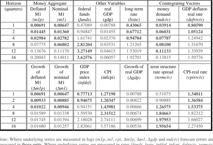
Table 7 (1/5/00) Vector Error Correction Model

Root Mean Square Forecast Errors at Various Horizons (formed over outsample period 1989:1–97:4)

Horizon Money Aggregate Other Variables Cointegrating Vectors (quarters) Deflated M1 (m1p) Nominal M1 (m1) federal funds (funds) real GDP (gdp) long-term rate (lrate) money demand (mdciv) GDP deflator-real rate (defrrciv) 1 0.00691 0.00647 0.47089 0.00788 0.43065 0.03914 0.80590 2 0.01445 0.01360 0.94847 0.01455 0.67712 0.06031 1.05124 4 0.02984 0.02782 1.61741 0.02376 0.94704 0.07787 1.24942 8 0.07775 0.06802 2.81204 0.03531 1.21265 0.08100 1.31670 12 0.13676 0.11170 3.27149 0.04615 1.53019 0.11133 1.33939 16 0.20043 0.14911 3.62576 0.06057 1.92701 0.13815 1.59776 Growth of deflated M1 (∆m1p) Growth of nominal M1 (∆m1) GDP price index (infdef) CPI (infcpi) Growth of real GDP (∆gdp) term structure rate spread (termciv) CPI-real rate (cpirrciv) 1 0.00691 0.00647 0.77713 1.27198 0.00788 0.51075 1.34011 2 0.00933 0.00885 0.94675 1.20347 0.00822 0.90885 1.36584 4 0.01022 0.00946 0.94151 1.43981 0.00666 1.26575 1.53375 8 0.01589 0.01338 1.59530 2.31512 0.00674 1.84663 1.82212 12 0.01745 0.01394 2.18028 2.74111 0.00699 1.97953 1.66027 16 0.01680 0.01257 2.82061 3.57186 0.00536 1.95654 2.27450 Note: Where underlying series are measured in logs (m1p, m1, cpi,∆m1p,∆m1,∆gdp and mdciv) forecast errors are measured in those units. Where underlying series are measured in rates (funds, lrate, infdef, infcpi, defrrciv, termciv, and cpirrciv), forecast errors are calculated as the difference between the forecast and actual rates, expressed as annual percentage rates of return.

Table 8 (1/4/00)

Univariate Random Walk Models

Root Mean Square Forecast Errors at Various Horizons (formed over outsample period 1989:1–97:4)

Horizon Money Aggregate Other Variables Cointegrating Vectors (quarters) Deflated M1 (m1p) Nominal M1 (m1) federal funds (funds) real GDP (gdp) long-term rate (lrate) money demand (mdciv) GDP deflator-real rate (defrrciv) 1 0.01222 0.01218 0.47040 0.00579 0.43135 0.05748 0.83838 2 0.02300 0.02272 0.84716 0.01040 0.70222 0.07596 1.07262 4 0.04253 0.04117 1.51744 0.01914 1.00651 0.09807 0.93735 8 0.07792 0.07056 2.81435 0.03450 1.14965 0.09452 1.01270 12 0.10472 0.08576 3.75252 0.04426 1.50643 0.11603 0.90339 16 0.12761 0.09234 4.00183 0.05267 1.61684 0.12688 1.31529 Growth of deflated M1 (∆m1p) Growth of nominal M1 (∆m1) GDP price index (infdef) CPI (infcpi) Growth of real GDP (∆gdp) term structure rate spread (termciv) CPI-real rate (cpirrciv) 1 0.01222 0.01218 0.81047 1.39678 0.00579 0.49564 1.41221 2 0.01214 0.01175 1.03071 1.55568 0.00589 0.84479 1.56529 4 0.01178 0.01076 0.83470 1.77866 0.00607 1.31282 1.76133 8 0.01256 0.01062 1.16595 1.95045 0.00572 2.02434 1.71659 12 0.01312 0.01059 1.58346 2.31526 0.00370 2.71034 1.38595 16 0.01105 0.01014 1.83126 2.74265 0.00372 2.74890 2.02375 Note: Where underlying series are measured in logs (m1p, m1, cpi,∆m1p,∆m1,∆gdp and mdciv) forecast errors are measured in those units. Where underlying series are measured in rates (funds, lrate, infdef, infcpi, defrrciv, termciv, and cpirrciv), forecast errors are calculated as the difference between the forecast and actual rates, expressed as annual percentage rates of return.

Figure 1

Recursive Residuals and Chow 1-Step Ahead Forecast Test Statistics (p-values for test of the null of stability measured on left hand scale of each panel)

0.15 0.10 0.05 0.00 -0.02 -0.01 0.00 0.01 0.02 84 86 88 90 92 94 96 0.15 0.10 0.05 0.00 -3 -2 -1 0 1 2 3 84 86 88 90 92 94 96 0.15 0.10 0.05 0.00 -2 -1 0 1 2 84 86 88 90 92 94 96 0.15 0.10 0.05 0.00 -4 -2 0 2 4 84 86 88 90 92 94 96 0.15 0.10 0.05 0.00 -0.03 -0.02 -0.01 0.00 0.01 0.02 84 86 88 90 92 94 96

One-Step Probability Recursive Residuals

0.15 0.10 0.05 0.00 -1.5 -1.0 -0.5 0.0 0.5 1.0 1.5 84 86 88 90 92 94 96

One-Step Probability Recursive Residuals

m1p infdef

funds infcpi

Figure 2

Recursive Residuals and Chow N-Step Ahead Forecast Test Statistics (p-values for test of the null of stability measured on left hand scale of each panel)

0.15 0.10 0.05 0.00 -0.02 -0.01 0.00 0.01 0.02 84 86 88 90 92 94 96 0.15 0.10 0.05 0.00 -3 -2 -1 0 1 2 3 84 86 88 90 92 94 96 0.15 0.10 0.05 0.00 -2 -1 0 1 2 84 86 88 90 92 94 96 0.15 0.10 0.05 0.00 -4 -2 0 2 4 84 86 88 90 92 94 96 0.15 0.10 0.05 0.00 -0.03 -0.02 -0.01 0.00 0.01 0.02 84 86 88 90 92 94 96

N-Step Probability Recursive Residuals

0.15 0.10 0.05 0.00 -1.5 -1.0 -0.5 0.0 0.5 1.0 1.5 84 86 88 90 92 94 96

N-Step Probability Recursive Residuals

m1p infdef

funds infcpi

Figure 3: VECM Forecast Errors 1990:1 - 1991:4

for three different estimation base periods

A: Growth rate of real GDP

90 91 -8 -6 -4 -2 0 2 4

B: Federal funds rate

90 91 -3 -2 -1 0 1 2 3 C: CPI inflation 90 91 -3.2 -2.4 -1.6 -0.8 -0.0 0.8 1.6 2.4 3.2

D: Growth rate of nominal GDP

90 91 -8 -6 -4 -2 0 2 4

VECM estimated through 1987:4 VECM estimated through 1988:4 VECM estimated through 1989:4

Figure 4: VECM Forecast Errors 1994:1 - 1995:4

for three different estimation base periods

A: Growth rate of real GDP

94 95 -2 -1 0 1 2 3 4 5

B: Federal funds rate

94 95 -5 -4 -3 -2 -1 0 1 C: CPI inflation 94 95 -3.5 -3.0 -2.5 -2.0 -1.5 -1.0

D: Growth rate of nominal GDP

94 95 -3 -2 -1 0 1 2 3

VECM estimated through 1991:4 VECM estimated through 1992:4 VECM estimated through 1993:4

Figure 5: GDP Growth Forecasts

Error Forecast 1990 0 1 2 3 4 5 6 7 8 error -3 -2 -1 0 1 2 3 1991 0 1 2 3 4 5 6 7 8 error -3 -2 -1 0 1 2 3 1992 0 1 2 3 4 5 6 7 8 error -3 -2 -1 0 1 2 3 1993 0 1 2 3 4 5 6 7 8 error -3 -2 -1 0 1 2 3 1994 0 1 2 3 4 5 6 7 8 error -3 -2 -1 0 1 2 3 1995 0 1 2 3 4 5 6 7 8 error -3 -2 -1 0 1 2 3 1996 0 1 2 3 4 5 6 7 8 error -3 -2 -1 0 1 2 3 1997 0 1 2 3 4 5 6 7 8 error -3 -2 -1 0 1 2 3 1998 0 1 2 3 4 5 6 7 8 error -3 -2 -1 0 1 2 3 FOMC Humphrey-Hawkins Council of Economic Advisors Blue Chip Economic Indicators Survey of Professional Forecasters

Macroeconomic Advisers (St. Louis) Fair Model

Random Walk VECM

Figure 6: Real Output Growth Forecasts

Error Forecast 1990 0 1 2 3 4 5 error -3 -2 -1 0 1 2 3 1991 0 1 2 3 4 5 error -3 -2 -1 0 1 2 3 1992 0 1 2 3 4 5 error -3 -2 -1 0 1 2 3 1993 0 1 2 3 4 5 error -3 -2 -1 0 1 2 3 1994 0 1 2 3 4 5 error -3 -2 -1 0 1 2 3 1995 0 1 2 3 4 5 error -3 -2 -1 0 1 2 3 1996 0 1 2 3 4 5 error -3 -2 -1 0 1 2 3 1997 0 1 2 3 4 5 error -3 -2 -1 0 1 2 3 1998 0 1 2 3 4 5 error -3 -2 -1 0 1 2 3 FOMC Humphrey-Hawkins Council of Economic Advisors Blue Chip Economic Indicators Survey of Professional Forecasters

Macroeconomic Advisers (St. Louis) Fair Model

Random Walk VECM

Figure 7: GDP Deflator Inflation Forecast

Erro r F o recast 1990 0 1 2 3 4 5 6 error -3 -2 -1 0 1 2 3 1991 0 1 2 3 4 5 6 error -3 -2 -1 0 1 2 3 1992 0 1 2 3 4 5 6 error -3 -2 -1 0 1 2 3 1993 0 1 2 3 4 5 6 error -3 -2 -1 0 1 2 3 1994 0 1 2 3 4 5 6 error -3 -2 -1 0 1 2 3 1995 0 1 2 3 4 5 6 error -3 -2 -1 0 1 2 3 1996 0 1 2 3 4 5 6 error -3 -2 -1 0 1 2 3 1997 0 1 2 3 4 5 6 error -3 -2 -1 0 1 2 3 1998 0 1 2 3 4 5 6 error -3 -2 -1 0 1 2 3 FOMC Humphrey-Hawkins Council of Economic Advisors Blue Chip Economic Indicators Survey of Professional Forecasters

Macroeconomic Advisers (St. Louis) Fair Model

Random Walk VECM

Figure 8: CPI Inflation Forecasts

Er ro r F o recast 1990 0 1 2 3 4 5 6 error -3 -2 -1 0 1 2 3 1991 0 1 2 3 4 5 6 error -3 -2 -1 0 1 2 3 1992 0 1 2 3 4 5 6 error -3 -2 -1 0 1 2 3 1993 0 1 2 3 4 5 6 error -3 -2 -1 0 1 2 3 1994 0 1 2 3 4 5 6 error -3 -2 -1 0 1 2 3 1995 0 1 2 3 4 5 6 error -3 -2 -1 0 1 2 3 1996 0 1 2 3 4 5 6 error -3 -2 -1 0 1 2 3 1997 0 1 2 3 4 5 6 error -3 -2 -1 0 1 2 3 1998 0 1 2 3 4 5 6 error -3 -2 -1 0 1 2 3 FOMC Humphrey-Hawkins

CEA Economic Report of the President Blue Chip Economic Indicators

Macroeconomic Advisers (St. Louis) Random Walk