The Appropriate Technology Frontier - Lessons for the Developing World

UNITED STATES NAVAL ACADEMY

DEPARTMENT OF ECONOMICS

WORKING PAPER 2007-16

“The Appropriate Technology Frontier - Lessons for the Developing World”

by

Ahmed S. Rahman Department of Economics United States Naval Academy

The “Appropriate” Technology Frontier

-Lessons for the Developing World

∗

Ahmed S. Rahman

Department of Economics

United States Naval Academy

Annapolis, Maryland

May 2008

Abstract

This paper presents a model of a developing economy that endogenizes both technological biases and demographic trends. As knowledge diffuses from foreign R&D-producing re-gions, potential innovators decide which technologies to develop after considering available factors of production, and individuals decide the quality and quantity of their children after considering available technologies. This interaction creates multiple growth paths. I find that if developing countries wish to achieve good prospects for income convergence, they should adopt fairly skill-intensive technologies, even if this initially creates a technology-skill mismatch. Such knowledge flows are more likely to promote the twin growths in human capital and technologies characteristic of the biggest economic success stories.

• Keywords: endogenous growth, demography, technological diffusion

• JEL Codes: O31, O33, J13, J24

∗_{Many thanks to Eran Binenbaum, Gregory Clark, Robert C. Feenstra, Petra Moser, Giovanni Peri, Katheryn}

N. Russ, Alan M. Taylor, Florence Bouvet, Chad Sparber, and participants at the 80th Annual Conference of the Western Economics Association, the Macro/International Brownbag Series at U.C. Davis, and the Meetings on Open Macroeconomics and Development at the Universit´e de la M´editerran´ee in Aix en Provence, France for many helpful suggestions. Naturally all errors are mine.

1

Introduction

The last half century has seen the robust growth of some nations and the persistent stagnation of others. This is particulary true of the developing world; while rich nations have maintained fairly consistent rates of growth (2 or 3% per annum), poorer nations have traversed widely different growth paths (between -1 and 7%). This paper suggests a possible reason behind such divergence by producing a model emphasizing the interdependence between directed technical change and demography. As general knowledge diffuses from foreign R&D-producing regions, potential innovators decide which technologies to develop after considering available factors of production, and individuals decide the quality and quantity of their children after considering available technologies. This interaction creates the possibility for multiple growth paths - some economies develop labor-intensive techniques and expand the pool of unskilled labor; others grow into societies of highly skilled individuals using sophisticated skill-intensive techniques. Which path will lead to greater prosperity is the primary focus of this paper.

The model emphasizes how dynamic inefficiencies can create such multiple paths. If the time horizon over which an individual maximizes utility is finite, cross-generational incentives may not be well aligned. These incentives are important for long-run growth in a world where education and skill-intensive technologies are strategic complements, and where education and unskilled-intensive technologies are strategic substitutes. If directed technological growth promotes skill accumulation in one generation, a virtuous cycle of technological and human capital growth can form for subsequent generations. If however innovation fosters population growth and limits education, technological growth can constrain the welfare of later generations and encourages similar behavior, resulting in a low growth trap.

This approach constitutes a notable departure from the existing literature on technologies that augment specific factors or sectors. These works often highlight the “inappropriateness” of growth in technologies that can be implemented by only a small portion of the economy. For example, Basu and Weil (1998) and Acemoglu and Zilibotti (2001) illustrate how technologies designed for capital-intensive (physical or human) societies that diffuse to developing regions are used ineffectually there, if at all. And Mokyr (1999) explains that the British Industrial Revolution initially produced only minor improvements in living standards because technical progress occurred in just a few small industries. These papers suggest that technologies catered for the abundant factors of production are more appropriate for the economy and will provide robust future growth.

But as we will see, allowing both factors and technologies to co-evolve changes the complexion of the problem, and alters the very meaning of what “appropriate” is. In the context of this treatment, I find that developing countries should promote the adoption of at least semi-skilled ideas from the knowledge frontier, irrespective of their own endowment levels. Although tech-nological progress in this case may be considered statically inappropriate for these economies’

large levels of unskilled labor, they may produce dynamically healthy incentives to invest and limit population growth, and hence improve living standards in the long-run. Thus taking an alternative route by promoting unskilled-intensive techniques may better employ the great pools of labor available in developing regions, but it will not produce the twin growths in human capital and technologies characteristic of the biggest economic success stories.

The rest of the paper is organized as follows. Section 2 refers to some past literature, and motivates the approach by looking at some cross-country data. Section 3 presents the full model in steps, first presenting a model of endogenous technological bias, and then merging this with a simple theory of demography. This model then motivates our discussion in section 4, which highlights the importance of skill-intensive technological growth both in general and in specific simulated examples. Section 5 provides some concluding remarks.

2

Accounting for Development

2.1

Past Literature

Growth economists often used to divide themselves into two distinct groups. One tended to to associate the accumulable factors of production (mainly physical and human capital) as the primary vehicles to prosperity (e.g. DeLong and Summers 1991, Mankiw, Romer and Weil 1992, etc.). The other group stressed technological differences across countries as the main source of income disparity (e.g. Romer 1990, Aghion and Howitt 1992, etc.). More recent studies however have begun to explore the simultaneity of “objects” (the factors of production) and “ideas” (technologies). For this paper I derive insight from three general branches of literature - papers where the ‘ideas’ of interest are factor-specific technologies, papers where the ‘objects’ of interest are different labor-types, and papers where the subject of interest is the interaction between the two.

Papers that analyze factor-specific technologies include Katz and Murphy (1992), Acemoglu (1998) and Kiley (1999), which attempt to explain rising skill-premia in developed countries, and Xu (2001), which attempts to explain international trade patterns. More related to this paper, a few studies have also explored biased technologies in the context of technological diffusion and development. These include Acemoglu and Zilibotti (2001), which compels developing countries to employ exactly the same technology as the developed one, and Caselli and Coleman (2000), which allows countries to choose the technology most appropriate to them given their factor supplies. However these studies all treat the factors of production as exogenously fixed.

Research on endogenous fertility, on the other hand, investigates how the micro decisions of households over the number of children and the level of education of each child can affect the macro economy. Becker and Lewis (1973) initiate this literature, while Becker and Barro (1988) develop a similar framework in a growth model; both cases model altruistic parents who make

consumption and fertility choices by maximizing a dynastic utility function. Moav (2005) models parents who decide both the number of children and the level of human capital of each child. Here instead of focusing on the potentialutility of their children, parents concentrate on the potential

income of their children. These models capture the quality-quantity tradeoff individuals face in

choosing their offspring, but remain silent on the technological environment.

Finally, theoretical models that considerinteractionsbetween endogenous technological change and skills include Stokey (1988), where innovations are the accidental by-products of learning by doing, and Chari and Hopenhayn (1991), where agents can use new technologies only by invest-ing in vintage-specific human capital. Other papers have endogenized both human capital and technological change, including Grossman and Helpman (1991), Young (1993), Redding (1996), Galor and Weil (2000) and Galor and Moav (2000). I build on this literature by also looking into the roles of directed technology and international knowledge diffusion.

2.2

A Cross-Section of Factor-Specific Technologies

If the research environment encourages the advancement of techniques used by the abundant inputs to production, we should have a sanguine outlook for the developing world. For example, a country awash in unskilled labor may simply develop and adopt labor intensive technologies, thus militating against anemic growth. Hence a world where each country can shape its technological destiny would be one where technologies are tailored to best suit the factoral composition of an economy.

In order to better appreciate this we attempt here to map out the efficiencies of different labor types for different countries. Consider then the following production function for country i.

Y = [(Al,iLi) σ

+ (Ah,iHi) σ

]1/σ (1)

Here we specify production as one with a constant elasticity of substitution skilled and un-skilled labor aggregates (this elasticity being 1/(1−σ). Al,i is the efficiency of unskilled labor in

countryi and AH,i is the efficiency of skilled labor in country i.1

Furthermore, if factors of production are paid their marginal products, the “skill-premium” may be written as:

wh,i wl,i = AH,i AL,i σ Hi Li σ−1 (2)

(1) and (2) represent 2 equations with 2 unknowns. That is, given data on Yi, Li, Hi, and wh

i

wl_i,

we can back out each country’s implied pair of technological coefficients in precisely the same

1_{This functional form resembles the production function used in section 3, where we endogenize technological}

fashion as Caselli and Coleman (2006).2

Key to this exercise is our parameter choice for σ ≤ 1. Careful empirical labor studies such as Autor et al (1998) and Ciccone and Peri (2005) have found that the elasticity of factoral substitution between more and less skilled workers most likely lies between 1 and 2 (consistent with a value ofσ between 0 and 0.5). We should add that when H is considered anyone with an 8th grade education or more,σ is likely to be higher for most countries. So both for this exercise and the simulations, we choose a benchmark value of σ = 0.5 for a proxy elasticity parameter most applicable for a wide range of countries and for a wide variety of skill-unskilled categories.3

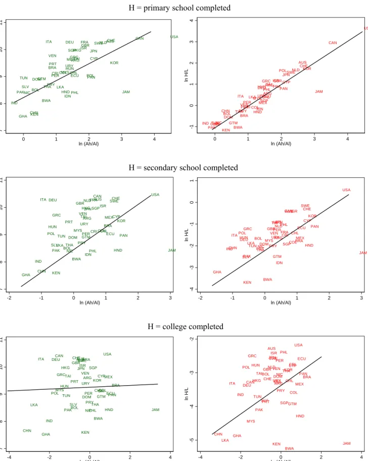
Table 1 reports these backed out measures of Al-Ah pairs. Figure 1 depicts the relationships

between relative technical skill-bias, relative skill-endowments, and income per capita across a broad array of countries. Immediately clear is the positive associations between skill-bias and skill endowment, and between skill-bias and income levels. These positive relationships hold whether we consider a skilled worker as someone who completed primary school, or someone who completed high school, or even someone who completed college. This was precisely one of the main points behind Caselli and Coleman’s study. Not only do wealthy nations enjoy large pools of human capital, but they also employ this capital far more effectively than poorer nations.

From these scatterplots emerge two puzzles. The first is the standard chicken-or-egg question. Does a country naturally endowed with a lot of human capital imitate/develop technologies best suited for this type of skilled workforce, becoming wealthy in the process? Or rather, does a country blessed for whatever reason with a rich pool of skill-intensive knowledge inherently provide the incentives necessary for growth in education? That is, is the path to wealth a technology story, or an investment story?

Second but no less a puzzle is the question of why un-skilled-intensive productivity fails to produce prosperity. According to standard directed technical change theories (see for example Kiley 1999, and Acemoglu 2002), if a country is populated primarily by the un- or under-educated, local innovators would simply direct their innovative energies toward technologies that would complement them. But the promise of symmetric opportunities for skill- and unskilled-intensive societies alike clearly fails to deliver in practice. Models which allow economic forces to endogenously shape technological direction thus add another layer of sophistication that shows more yet explains less.

This paper suggests that theco-evolution between factors and technologies may in part explain these puzzles. Skill-bias knowledge and human capital may reinforce each other, just as

unskilled-2_{The data is also from Caselli and Coleman (2006). Y is average GDP per capita for 1985-1990, taken from the}

Penn World Tables. Labor levels are constructed using the implied Mincerian coefficients from Bils and Klenow (2000). Wages for skilled and unskilled are constructed using Mincerian coefficients and the duration in years of the various schooling levels. See their paper for more details.

3_{Ciconne and Peri (2005) themselves estimate σ to be 0.5 when considering U.S. high school dropouts as}

bias knowledge and unskilled labor may reinforce each other. If the composition of the economy is what is most crucial (so that the large sectors of the economy are the ones that grow fastest), then either path will create robust growth. But if there are negative dynamic consequences for unskilled-intensive development (such as population growth), then per capita growth from unskilled bias technological change will be muted. Thus a model of virtuous and vicious cycles may explain not only the scatter diagrams of Figure 1, but the general observation that poorer countries have experienced wildly different growth rates in the last 50 years. These ideas are made more concrete in the model of section 3.

2.3

A Cross-Section of Demographic Characteristics

Along with a combination of technologies, a country chooses a combination of factors through household decisions on education and procreation. A cross-country sample of these decisions are depicted in Figure 2. Here observations are sized according to the country’s income per capita. We can observe a negative correlation between population growth and education, a negative correlation between population growth and living standards, and a positive correlation between education and living standards.

It is also commonly believed that child labor is a symptom of poverty (Edmonds and Pavcnik 2005). This should be important to us, since a child working is a child not in school. The International Labor Organization’s Statistical Information and Monitoring Program on Child Labor (SIMPOC) most recently estimated that 211 million children, or 18% of children 5-14, are economically active worldwide (ILO 2002). Figure 3 illustrates the strongly negative relationship between living standards and the percentage of 10-14 year-olds who are employed.

Thus we observe that prosperity is associated with low fertility rates, high education rates, and low child-labor participation rates. Further, from our observations in the previous section, we can say that these characteristics are also associated with high relative efficiency levels of skilled labor. The theory in the following sections will combine these observations. While these scatter diagrams are cross-country representations taken at only one moment in time, we might speculate on what economic developments led up to these relationships. As such we view these static pictures as the primary impetus to develop a dynamic model of growth.

3

The Model

In this section we present a simple model where global knowledge flows spur local factor-specific invention. Subsection 3.1 illustrates the production side of the economy. Subsection 3.2 illustrates the research and technology adoption side. Subsection 3.3 merges this approach with a simple theory of demography; the combined model allows us to evaluate the co-evolution of

factors and technologies so that we can judge in the next section the true “appropriateness” of different kinds of technological developments.

3.1

Production

Consider a discrete-time economy. We use the production function given by (1) but now we explicitly specify factor-specific technologies. Specifically production is specified as the following.

Y = [(AlL) σ + (AhH) σ ]1/σ (3) Al≡ Z Ml 0 xl(j) L α dj Ah ≡ Z Mh 0 xh(k) H α dk (4)

Here both types of labor (unskilled L, and skilled H) work with intermediate “machines” to produce a homogenous final output. I make the rather stringent assumption that these machines can complement either skilled labor or unskilled labor, but not both. Machines (of type j) which complement unskilled labor are denoted by xl

j, while machines which complement skilled labor

are denoted by xh_j.

The parameter σ indicates the degree of substitutability between skill and unskill-intensive “sectors” in aggregate production. When σ = 1, the production function is linear; when it is 0, the production function is Cobb-Douglas; when it is −∞, the production function is Leontieff. As we mentioned in section 2.2, estimates of this elasticity clearly place σ above zero; thus we will assume that these sectors are grossly substitutable, so unbalanced growth (progress that is confined to just one of the sectors) can still produce growth overall. Indeed, we see such unbalanced growth stories throughout the world. For example, a farm in India likely employs many uneducated workers using scythes, while a farm in Western Europe probably employs a few workers skilled at using sophisticated agronomic instruments. This characterization of different labor-types using different types of machines, or “production processes,” with which these labor types are compatible seems a reasonable approximation for actual technological biases.

Technological advance is assumed to come in two varieties. In the “unskilled labor sector,” technical advance comes about from an expansion in the number of intermediate machines spe-cialized for unskilled labor (that is, an increase in Ml). Similarly, in the “skilled labor sector,”

technical advance means an expansion in the number of intermediate machines specialized for skilled labor (an increase in Mh).

Final goods output produced by different firms is identical, and can be used for consumption, for the production of different intermediate machines, and for research and development to expand the varieties of skill-augmenting and unskilled-augmenting machines. For each time period (suppressing time subscripts for the moment) these firms endeavor to maximize:

max {L,H,xl(j),xh(k)} Y −wlL−whH− Z Ml 0 p(j)xl(j)dj − Z Mh 0 p(k)xh(k)dk (5)

Intermediate machines, on the other hand, are produced either in monopolistic or competitive environments. Specifically, an inventor of a new machine at time t−1 enjoys monopoly prof-its for machine production at t. After this, however, patent rights to this machine expire, and subsequent production is performed by many competitive manufacturers. Whether a machine is produced monopolistically or competitively will be conveyed in its rental price, denoted either as p(j) for a unskilled-labor using machine j or p(k) for a skilled-labor using machine k, and explained in the next sub-section. For simplicity, we assume that all machines depreciate com-pletely after use, and that the marginal cost of production is simply unity in terms of the final good.

Assuming for the moment that both technology levels Ml and Mh and labor types L and H

are given, an equilibrium can then be characterized as machine demands for xl(j)’s and xh(k)’s

that maximize final-good producers’ profits (from equation 5), machine pricesp(j) andp(k) that maximize machine producers’ profits, and factor prices wl and wh that clear markets.

The first-order conditions for final-good producers yield intermediate-machine demands:

xl(j) = [(AlL) σ + (AhH) σ ] 1 −σ (1−α)σ _A 1−σ α−1 l p(j) α _α−1₁ Lσ−α1−α xh(k) = [(AlL) σ + (AhH) σ ] 1 −σ (1−α)σ _A 1−σ α−1 h p(k) α _α−1₁ Hσ−α1−α ₍₆₎

Note that here a greater level of employment of a factor raises the demand for intermediate goods augmenting that factor so long as σ > α, an idea consistent to what Acemoglu refers to as a “market-size effect.” We will assume throughout the analysis that this condition is met.

The other first-order conditions for final-good producers illustrate that workers receive their marginal products: wl = [(AlL)σ + (AhH)σ] 1−σ σ _Aσ lL σ−1 wh = [(AlL)σ + (AhH)σ] 1−σ σ _Aσ hH σ−1 ₍₇₎

3.2

Research

In this section we endogenize the growth paths of Ml and Mh. Local researchers expend

re-sources to develop new types of machines, but they will be heavily influenced by the international flow of knowledge. We make these modeling choices to stress that the nature of technological

growth for developing countries depend both on local conditions and technological diffusion from advanced countries.

With regard to the time required to develop a new machine, assume that it takes one period from when the costs of development are incurred to when the machine can be monopolistically produced and sold. With regard to the costs of development, these will depend both on the number of machine types already extant (indexed by Ml and Mh), and on the current level of

factor-specific frontier knowledge (denoted by Ωl and Ωh, and discussed below). Thus the costs

of innovation are allowed to evolve in this economy. Specifically, the up-front cost of developing the blueprint of a new machine is given by

c Ml Ωl = Ml Ωl φ

for an unskilled labor augmenting machine, and

c Mh Ωh = Mh Ωh φ

for a skilled labor augmenting machine, with the assumption that φ >1. These functional forms illustrate that the costs of invention are negligible when frontier technologies are far advanced relative to “local technologies.” As local technologies begin to outstrip frontier technologies, however, costs become increasingly prohibitive.4.

Given these costs of technological advance, innovating firms must receive some profits from the development of a new technology in order to make research and development worth the expense. As mentioned above, we assume that developers of new machines receive monopoly rights to the production and sale of their machines for only one period. As a result, we must make a distinction between old machines (those invented before t) and new machines (those invented at

t).

The rate of interest with which profits are discounted are pinned down by consumers’ pref-erences. However, we lose no insight if I treat the interest rate simply as the time discount factor. Assuming unitary marginal costs of machine production, the steady-state present values of profits from new machines of both classes are given by:

Vl,t = (pt+1(j)−1)xl,t+1(j)· 1 1 +r Vh,t = (pt+1(k)−1)xh,t+1(k)· 1 1 +r

4_{This approach of varying the cost of research based on distance from the frontier of knowledge echoes the}

Because demand is isoelastic, the price which maximizes monopolists’ profits equals 1/α for both skill- and unskilled-augmenting machines, so that demand for new intermediate machines are notated simply as:

xl,new(j) =xl,new =α 2 1−α [(A lL)σ + (AhH)σ] 1−σ (1−α)σ _A 1−σ α−1 l L σ−α 1−α xh,new(j) =xh,new =α 2 1−α[(A lL)σ+ (AhH)σ] 1−σ (1−α)σ _A 1−σ α−1 h H σ−α 1−α (8)

On the other hand, because older machines are competitively produced, their prices equal unitary marginal costs, so that curves for old intermediate machines are:

xl,old(j) =xl,old =α 1 1−α[(A lL)σ+ (AhH)σ] 1−σ (1−α)σ _A 1−σ α−1 l L σ−α 1−α xh,old(j) =xh,old =α 1 1−α _[(A lL) σ + (AhH) σ ] 1 −σ (1−α)σ _A 1−σ α−1 h H σ−α 1−α ₍₉₎

Thus factor-specific TFPs given by equation (3) can be re-written as an aggregation of two kinds of machines - old and new:

Al ≡ Z Ml 0 xl(j) L α dj = " Z Ml,old 0 xl,old(j) α dj+ Z Ml,new Ml,old xl,new(j) α dj # (1/L)α =

Ml,oldxαl,old+Ml,newxαl,new

Lα (10) Ah ≡ Z Mh 0 xh(k) H α dk = " Z Mh,old 0 xh,old(k)αdk+ Z Mh,new Mh,old xh,new(k)αdk # (1/H)α =

Mh,old xαh,old+Mh,newxαh,new

Hα (11)

Substituting (8) and the monopoly price into our valuation functions yield the present values:

Vl,t = 1−α α xl,new 1 1 +r Vh,t = 1−α α xh,new 1 1 +r

wherexl,new and xh,new are given by (8). An individual is free to research, guaranteeing that:

Vl,t(Lt+1, Ht+1, Al,t+1, Ah,t+1)≤c Ml,old+Ml,new Ωl,t (12)

Vh,t(Lt+1, Ht+1, Al,t+1, Ah,t+1)≤c Mh,old+Mh,new Ωh,t (13) where of course Mz,old+Mz,new = Mz,t for factor z (that is, factor-specific technology is the

cumulation of all past innovation and all new innovation). If resource costs of research were actually less than discounted profits, entry into research would occur, driving local technology levels, and hence costs, up. I assume this happens quickly, so that valuations never exceed costs in any time period. Further, since applied research is irreversible (a society cannot forget how to make something once it is learned), the variety of machines remains unchanged when the inequalities in (12) or (13) do not bind with equality.

The levels of frontier knowledge in the economy are key determinants of the costs of developing new “production processes;” higher levels of Ωz lower the costs of developing intermediate

ma-chines which complement factorz. Conceivably these technological levels arise from the research output of other more developed economies; as such we can consider the growth of Ωl and Ωh as

exogenous to our economy of interest. Furthermore, countries which produce the most amount of technological output (and thereby which are most likely to influence the developments of ΩL_and

ΩH_{) are those countries most likely already in their steady-states. As a result I allow reference}

technologies to simply grow at an exogenously steady rate:

g = Ωl,t+1−Ωl,t Ωl,t

= Ωh,t+1−Ωh,t Ωh,t

where g > 0 is the growth factor.5 _{Thus we see that (12) and (13) also capture our notion}

of barriers to technology adoption - if Ωl and/or Ωh are too small, factor-specific technological

growth cannot happen. Indeed the economy cannot begin to technologically grow until this “reference technological frontier” is sufficiently developed.

The steady-state can be characterized as one where the share of labor devoted to each sector (skilled and unskilled) remains fixed, while output, the stock of basic research knowledge, the varieties of skilled and unskilled complements, and wages all grow at the same rate, g. This will occur so long as equations (12) and (13) hold with strict equality. But as these equalities imply there may be a considerable period of time when growth is unbalanced; this would occur if only one of the equations held with equality. What kind of unbalanced growth is likely to unfold will depend on a number of things, including the available supply of different factors (a relatively large L for example raises Vl and thus increases the chance that growth will be unskill-biased)

and the relative “skewness” of the knowledge frontier (a relatively large Ωl for example lowerscl

and likewise increases the chance for unskill-biased growth).

5_{Subsequent work may endeavor to endogenize the evolution of this “frontier” knowledge. Note here however}

that the recent skill-biased technical change literature suggests that Ωh has grown faster than Ωl, particularly

throughout the 1980s and 90s (Acemoglu 2002; Goldin and Katz 2007). This would only reinforce our suggestion that skill-intensive growth is the superior path to development; as such I wish not to rely on this assumption.

Clearly unbalanced growth is slower than balanced steady-state growth, but surely growth in the bigger sector will produce faster growth overall.6 _{This indeed is the essence of the}

ap-propriate technology story - typically it involves a story of factor abundance. By its logic, a country awash with throngs of unskilled labor would do well to develop and adopt technologies readily employable by them. The tragedy stressed in this tale often involves the nature of the technology frontier - because cutting-edge technologies produced by wealthy nations tend to be skill-intensive, developing nations face a large (Ωh/Ωl); consequently they are forced to adopt

technologies for which they are structurally ill-suited, resulting in anemic growth in general.7

Yet compelling as the appropriate technology story is, we would feel delinquent of duty to end the tale there. The symmetrical opportunities on display in this model belie the reality so transparent from Figure 1 - countries that do have a relatively large unskilled workforce do make them relatively more productive. But countries do not get wealthy that way. The simple model on display here thus seems to miss some notable aspects of growth - countries seem able to “shape” their own knowledge frontier in such a way as to adopt technologies for their abundant factors, but such a shift towards unskilled-intensive growth seems not to produce much per capita growth. Why not?

We would suggest that incentives to change the factors of production themselves may be an important part of the answer. Specifically, changes in the relative rewards to factors due to technological developments surely will alter the incentives to accumulate education or to remain an unskilled laborer. From the model we can write the “skill premium,” the skilled wage relative to the unskilled wage, as

wh wl = α α 1−αM h,old +α 2α 1−αM h,new α1−αα M l,old+α 2α 1−αM l,new !σ−σα₁−σα · H L ₁σ−_−σα1 (14) In the absence of any demographic response, skill-bias technological growth will raise the skill premium (by raising Mh,new), while unskill-bias technological growth will lower it (by raising

Ml,new). But surely if unskill-intensive growth lowers the relative returns to skill, this will induce

people to remain unskilled and so not accumulate human capital. The question we now want to ask is if this model can be combined with a fairly simple model of demography that can capture this idea. The next section endeavors to do precisely that.

6_If ∆a a =gand ∆b b = 0, ∆(a+b) a+b = ∆a

a+b, which is smaller than, but converges to, g. The smaller is b relative to

a, the closer will this growth be to g.

7_{The development literature is filled with anecdotal evidence of this technology-skill mismatch, highlighted in}

Todaro and Smith’s seminal text. “Gleaming new factories with the most modern and sophisticated machinery and equipment are a common feature of urban industries while idle workers congregate outside the factory gates.” (pp. 256 in Todaro and Smith 2006).

3.3

Endogenous Demography

What if individuals were allowed to respond to changes in the technological landscape? Eco-nomic forces after all tend to heavily shape the demographic composition of a society. At the same time (as modeled in the previous section), technological developments tend to follow the fac-tors that can implement them, and so are strongly shaped by demographic composition. Thus, we can conceive of a simultaneous solution model which embodies this symbiotic relationship between technologies and resources.

Here we explore this possibility by extending the core model in the following fashion. We now adopt an over-lapping generations framework where individuals have three stages of life: young, mature, and old. Only mature adults are allowed to make any decisions regarding demography. Specifically, the representative household is run by an adult who decides two things: how many children to have (denoted nt) and the level of education each child is to receive (denoted et).

The modeling arrangement is now as follows. An individual born at time t spends fraction

et of her time in school (something chosen by her parent), while devoting the rest of her time

as an unskilled laborer. At t+ 1, the individual (who is by this time a mature adult) works

strictly as a skilled laborer, utilizing whatever human capital she had accumulated as a child in the skilled sector. At this stage she also decides the quantity and quality of her children (nt+1

and et+1, respectively), and sets them out to toil as unskilled workers. After incurring the costs

of child-rearing, the adult consumes all the income she and her family have generated, but only after she has distributed a set fraction of her skilled-income to her parent. No credit markets exist, so adults consume all surplus production. At t+ 2, the individual is old, does not work, and consumes only what is redistributed to her by her children. After this the individual expires and exits the economy.

This 3-stage OLG framework is most appropriate for developing nations, whose children often work instead of go to school, and whose elderly often require care from their grown children. Further, in the absence of well-defined capital markets, education serves as a metaphor for capital, and therefore as a tool of investment. An adult who invests in the “quantity” of children will earn a return relatively quickly (through increased unskilled income), while one who invests in the “quality” of children must wait before there is a payoff (through the redistribution of future skilled income).8

Given all this, let us specify a utility function which a mature adult will wish to maximize. For the individual born at time t, utility can be written as:

8_{We could allow adults to continue to work as unskilled laborers if they would earn more doing so. In this case}

whatever human capital they had accumulated would be left idle. However, given parameter values and initial conditions in the simulations, an adult will always earn more as a skilled worker, and so will always be one if given the choice.

Ut+1 =C1t+1+

1

1 +rC2t+2 (15)

where C1t and C2t denote the consumption in period t of adults and the elderly, and r is the

discount rate. Thus I maintain the assumption (for simplicity) that agents are risk neutral, and are strictly motivated to increase the present value of their income regardless of when they receive it.

From the discussion above, I define consumption streams as follows:

C1t+1 = [1−τ]wh,tH(et−1) +wl,tnt[1−et]−wh,tϕ(nt, et)

C2t+2 =τ wh,t+1H(et)nt

where H(·) is the production function for skills, ϕ(·) is the time required to raise children, τ is the fraction of skilled-income that an adult must relinquish to his elderly parent, and wageswl,t,

wh,t and wh,t+1 are determined by (7). Thus the individual born at time t−1 will choose the

pair {nt, et} that maximizes (15).

Note that the skilled wage for next period, wh,t+1, will depend on technological coefficients

which are determined by researchers this period. Families therefore decide the demographical variables by solving (15) taking technological coefficients as given, while researchers determine tech coefficients by following either (12) or (13) taking demographic variables as given. Finally note that the fertility rate nttranslates directly into the pool of unskilled laborthis period, while

education rate et translates into the pool of skilled labor next period. Thus solving (12), (13)

and (15) simultaneously at every moment in time allows us to generate a path of demographic and technological variables.

The first-order condition for the number of children is:

wl,t[1−et] + τ 1 +rwh,t+1H(et) =wh,t ∂ϕt ∂nt (16) The left-hand side illustrates the marginal benefit of an additional child, while the right-hand side denotes the marginal cost. At the optimum, the gains in income from an extra unskilled worker in the familyand an additional source of retirement income precisely offsets the foregone skilled-income that results from child-rearing.

The first order condition for education is:

wl,tnt+wh,t ∂ϕ ∂et = τ 1 +rwh,t+1nt ∂H ∂et (17) Here the left-hand side is the marginal cost and the right-hand side the marginal benefit. At the optimum, the gains received from the added retirement income at t+ 1 offsets the foregone unskilled- and skilled-income requisite for an additional unit of education for all children at t.

Completing the model requires functional forms forH(·) and ϕ(·). In order to have a globally convex problem, I specify the following:

H(et) = Θekt

ϕ(nt, et) = nt(1 +et)

β

With these simple functional forms, we can propose the following:

Proposition 1 If 0< k <1 and β >1, ∂e∗_t ∂Mh,t >0 → ∂Ht+1 ∂wh wl >0 ∂n∗_t ∂Mh,t <0 → ∂Lt ∂wh wl <0

That is, if there are diminishing returns to education and convex costs of child rearing, an adult who observes a widening skill premium will not only endow her children with more education (thus increasing H), she will also reduce her number of children (thus decreasing L). For an un-rigorous “visual proof” of this, see Figure 4.

Combining this model of demography with our model of biased technologies is straightforward. Through the simultaneous solving of (10), (11), (12), (13), (16) and (17), a unique set of variables

Lt(n∗t),Ht+1(e∗t),Mh,t,Ml,t,Al,t andAh,t is determined for every time periodt. We can perhaps

synopsize our findings by initially focusing only on the choice of e∗_t and Mh,t. If an adult expects

researchers to currently develop new skill-biased technologies for future implementation (and so to increase wh,t+1), she will want to endow her children with more human capital. Similarly,

if researchers anticipate a larger pool of human capital in the future, they may wish to expand their research of skill-biased technologies. Consequently we can plot the two “reaction functions” of each group as two upward-sloping curves; the development of new skill-using machines and the accumulation of skills are strategic complements. From the intersection of these reaction curves we find the unique simultaneous solution of the level of education and the new skill-biased technical coefficient. This is done in Figure 5. Furthermore, each et corresponds to a unique nt

(depicted by the intersection of the the first-order curves in Figure 9).9

To summarize, potential researchers look to the skill composition of the workforce (something that is shaped by households) to determine the direction and scope of technical change. Further, households look to relative wages (something that is shaped by researchers) to determine the levels of skilled and unskilled workers. Accordingly I do not take a stand on the direction of

causality between technology composition and labor composition. Since our model is built on an overlapping generations framework (so that successive time units are at least a decade apart), we may plausibly say that both occur simultaneously within a given interval of time.

4

”Appropriate” Growth Paths for a Developing Country

- Two Experiments

Now that we have a model that endogenizes the growth paths of both technologies and factors, we may better assess the appropriateness of alternative development paths. Let us consider a hypothetical developing country endowed with a lot of unskilled labor but little human capital. Given this demographic composition, unskilled-bias technological growth will conceivably aug-ment a large part of economy and therefore substantially contribute to overall growth. Let us call this thecomposition effect of technological change. At the same time, Proposition 1 suggests that such unskilled-intensive growth will raise fertility rates and lower education rates by putting downward pressure on the skill premium. Let us call this thecapita effect of technological change. The question we want to ask is: Are there plausible scenarios where the positive composition effects fail to outweigh the negative capita effects of unskilled-intensive growth?

We answer in the affirmative by having two thought experiments. First, we perform a nu-merical exercise by comparing different changes in the economy, using the lessons of the model. Second, we perform a numerical exercise by dynamically simulating the model itself. These experiments constitute the next two sections of the paper.

4.1

Unbalanced Growth - A Comparative Static Experiment

One of the main lessons of the model is that technological progress involves changes to both technologies and factors. To better judge these effects, let us totally differentiate the per capita version of the production function given by (1):

dy+dL= ∂y ∂Al dAl+ ∂y ∂Ah dAh+ ∂y ∂L dL+ ∂y ∂H dH (18)

Both types of technologies and both types of factors have the potential to change. Notice the dL term on the left hand side, which is there to suggest that changes in unskilled labor is tantamount to changes in population. While this is in fact what the model suggests, strictly of course this is not true. However, in a world of no labor migration or obsolescence of skills, changes in unskilled labor and population should be highly correlated; therefore dL is a fair approximation for both changes in population and changes in unskilled labor.

When there is unskill-biased technological change, the total change in income per capita can be written as

dyunsk+dL= [(AlL) σ + (AhH) σ ]1 −σ σ _{· (A} lL) σ−1 (L·dAl+Al·dL) + (AhH) σ−1 (Ah·(−dH)) (19) where dyunsk is the total change in income per capita with unskilled intensive growth. Here we

assume that Ah does not change (hence dAh = 0) and that this type of technological growth has

de-skilling effects (hence the negative sign in front of dH). On the other hand, when there is skill-biased technological change, the total change in income per capita can be written as

dysk −dL= [(AlL) σ + (AhH) σ ]1−σσ · _(A lL) σ−1 (Al·(−dL)) + (AhH) σ−1 (Ah·dAh+ (AhdH)) (20) where dysk is the total change in income per capita with skilled intensive growth. Here we

assume that Al does not change (hence dAl = 0) and that this type of technological growth has

anti-fertility effects (hence the negative sign in front ofdL).

We want to know whether or not unbalanced unskill-intensive growth is better than unbalanced skill-intensive growth. That is, we ask if dyunsk > dysk? Setting dAl =dAh =dL =dH = 1 (so

that changes in factors and technologies are symmetrical) and rearranging this condition a bit gives us the following condition:

Proposition 2 Unbalanced unskilled-intensive growth will be faster for overall growth than

un-balanced skill-intensive growth (that is, dyunsk > dysk) if and only if

AhH AlL 1−σ ·(L+ 2Al)−2 (AhH)1 −σ H+ 2Ah >1

This simply states that the unskilled sector must be sufficiently large relative to the skilled sector in order for unskill-intensive growth to produce more per capita output than skill-intensive growth. Notice that these relative sizes depend not just on factor endowments (L and H), but also how effective these factors are in production (Al and Ah).

To test whether or not Proposition 2 holds for most countries, we require cross-country data on L and H (which once again we have from Caselli and Coleman 2006), Al and Ah (which we

back out from equations (1) and (2), and a choice for the value of σ. Based on our discussion in section 2.2, we use bothσ = 0.33 and σ = 0.5.

Table 2 reports our findings. With the exception of Jamaica, we see thatdyunsk< dysk for each

the majority of our countries only whenH is considered those with a primary school education or more. The difference arises because when the skilled and unskilled sectors are more substitutable, the unskilled sector is not much larger than the skilled sector (this is because Ah and Al are

fairly close to each other in value); in this case the positive composition effects of unskilled-bias growth do not offset the negative capita effects, even when H is narrowly categorized as college graduates. On the other hand, more complementarity between the sectors pulls Ah and

Al further apart; as such the skilled sector becomes much smaller, and so composition effects

tend to dominate capita effects as our categorization ofH gets narrower.

We thus conclude that there are indeed plausible cases when skill-biased growth leads to more per capita output growth, even among the poorest and most unskill-labor abundant countries. The capita effects will tend to offset the composition effects of unbalanced growth the greater is the elasticity of substitution between unskilled and skilled labor, and the broader is our definition of skilled labor.10

4.2

Unbalanced Growth - A Simulation Experiment

The above exercise tests the effects of unbalanced growth in a general and comparative static way. However, we may also wish to know the dynamic implications of the specific model delin-eated in section 3. That is, by actually endogenizing the micro-economic incentives for researchers and families, we can generate actual values for dAl, dAh, dL and dH over time.

Further, the model also suggests a relationship between the “technological frontier” that a country faces and its own prospects for growth. Specifically, by equations (12) and (13) we see that the more skewed is the technological frontier towards skilled-oriented knowledge, the greater is the likelihood that the early stages of growth for the developing country will be skill-intensive. While we do not endeavor to endogenize the skewness of the frontier, we should acknowledge how this skewness relates to our hypothetical economy’s relation to the developed world. For example, a “technologically open” economy would have access to the most highly advanced knowledge produced in the world - given that most basic research takes place in the highly skill-endowed G-5 countries (Jones 2002), this openness will most likely raise (Ωh/Ωl). On the other

hand, a relatively closed-off society would likely not only have lower levels of both Ωl and Ωh (so

that economic takeoff will be delayed), but also have a lower (Ωh/Ωl) (so that when economic 10_{Note that the liberal definition of skilled labor would be most appropriate for precisely those under-developed}

economies on which we are focussed.

11_{A note on parameterization here: the lessons of the simulation story require the following parameter}

restric-tions - 0 < τ < 1, 0 < α < σ < 1, 0 < k <1, Θ > 0, and β > 1. In words, this simply means that people discount the future, there are diminishing returns to machines and education, skilled and unskilled labor types are grossly subtitutable, there is a positive coefficient for “human capital production,” and there are rising costs for child-rearing. So long as these basic restrictions are met, the overall conclusions that follow the simulations will hold.

growth does occur, it is more likely to be unskill-intensive).

The end lesson perhaps is that there are many things an under-developed nation can do to shape its technological frontier - the question for us is what would be the appropriate shape, one where (Ωh/Ωl) is small, or one where it is large? This is simply another way of asking if

dyunsk> dysk - if so we should want a relatively low (Ωh/Ωl), for skill-intensive growth would be

inappropriate for such an economy.

To answer these questions, we simulate a few scenarios of the full model, varying only ini-tial levels of L and H and the initial position of the reference technological frontier ΩH_/ΩL_.12

Specifically, we consider an economy with a relatively high initial endowment of H/L = 0.5 (in line with a country like India when we considerH as those with a primary education or more, or a country like South Korea when we consider H as those with a secondary education or more), which we call Economy A, and an economy with a relatively low initial endowment of H/L = 0.25 (in line with a country like Kenya whenH is considered those with a primary education or more), which we call Economy B.13

All other parameters (enumerated at the bottom of Figure 6) are the same for all simulations - all we vary are the technological frontier and the factoral endowments of our hypothetical developing economy. For all cases we run the simulation for 30 time periods. The technological frontier exogenously expands out in an even fashion (Ωl and Ωh grow at the same rate g) and

our developing economy responds to these changes.

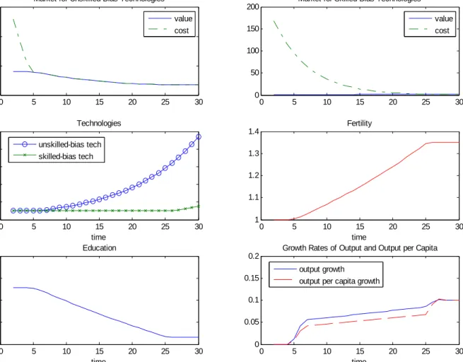
The case we show in Figures 6 and 7 is Economy A - this economy has the relatively high ratio of skilled to unskilled labor of 0.5. For the simulation of Figure 6 we set values for Ωl and

Ωh so that unskilled technologies are the first to develop, and this happens at t = 5. At t=27,

near the end of the simulation, Ωh has grown such thatMh finally begins to grow as well. At this

point both sectors expand the number of machines used, and growth is finally balanced. Notice that during the period of unbalanced growth, fertility rates rise and education rates fall; this is because as unskilled technologies grow, the skill premium falls, and this induces households to respond demographically through Proposition 2. As a result, growth in output per capita is lower than growth in overall output until balanced growth is achieved.14

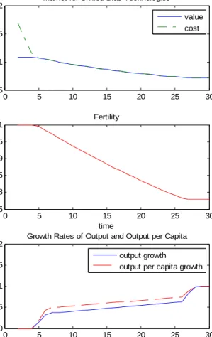
For the economy of Figure 7 we reverse this experiment. That is, we set Ωl and Ωh such that

the skilled sector begins to grow at t=5, and the unskilled sector grows at t=27. This produces

the opposite demographic response - fertility rates fall and education rates rise. In this case then unbalanced growth produces faster per capita growth than overall output growth.

12_{nis normalized to 1 at the start of each simulation to maintain a constant population.}

13_{Again, see the Caselli and Coleman (2006) study for how the data forL andH is constructed.}

14_{Those dissatisfied with such imbalanced growth may do well to recall the words of Abramovitz and David}

(1973): “...economic growth as we have known it is not a balanced steady-state affair in essence...Rather, central features of the historical process of growth since the earliest years of the Republic may be viewed as part of a sequence of technologically-induced traverses, disequilibrium transitions between successive growth paths.”

Thus we see that unskilled growth produces lower per capita growth but affects a larger part of the economy, while skilled growth produces higher per capita growth but affects a smaller part of the economy. In order to judge which unbalanced growth path is superior, we need to compare per capita growth income for each case. In this fashion, we can pit the two growth paths against each other and see which one comes out ahead. The top portion of Figure 8 shows the results of this race. It is clear that for this endowment structure, skilled growth is “better” - the positive capita effects offset the negative composition effects.

However, for economy B where H/L is set to 0.25, we reach a different conclusion. For each kind of technological frontier, we get very similar fertility, education and income paths as Economy A (not shown). However, in this case the positive capita effects of skill-intensive growth tend not to offset the negative composition effects over time - the unskilled sector in this case is simply too large. This is illustrated at the bottom of Figure 8. Here unskill-intensive technological growth is indeed the superior growth path.

The fact that economy A performs better under skill-intensive growth than unskill-intensive growth introduces an alternative interpretation of what is appropriate in technological growth. The strategic complementarity between skill acquisition and skill-biased technical development underscores the possibility of virtuous cycles of technology growth and accumulation. Here skill-biased technologies are inherently superior not because they augment a large portion of the economy (neither for economy A nor B is the skilled sector larger than the unskilled sector) but rather because they provide families with the incentives to accumulate human capital and limit fertility. As such economies which face a technological frontier skewed towards the skilled are likely to benefit from growing skill-intensive techniques even if they are heavily endowed with unskilled labor.

The slower growth prospect for economy A with unskill-bias growth is simply the by-product of

adynamic inefficiency. Agents of each generation do not concern themselves with the long-term

welfare implications of their demographic decisions. The myopia inherent in the inter-temporal structure of the economy is not quite as harmful when skill-biased techniques are developed, for then cross-generational incentives are better aligned. But when unskilled-biased techniques are the first to grow, this myopia can prove to be an anchor for growth; the incentive that spurs the agent to have more children with less human capital leaves the next generation worse off, and gives them little choice but to do the same.

However, we must acknowledge that these dynamic effects may not prove to be so disastrous, depending on the relative size of the unskilled workforce and their current productivity. If for example we consider a skilled worker only those with a college degree or more, then the “skilled sector” may be so small that adopting technologies for this labor type will not produce much benefit. Indeed this is the case of our simulated economy B.

as equally beneficial. A nation thronging in unskilled labor may initially find it in its interest to have a low ΩH_/ΩL _{and thus allow it to develop labor-complementary techniques. But such}

developments may leave individuals with little incentive to invest in education. A country on such a path could find itself in a vicious cycle of rising population and slower output per capita growth, even as it implements new technologies all the while. This may in part explain why poor countries can not seem to alleviate their poverty simply by improving unskilled-intensive techniques.

5

Conclusion

This paper has suggested the existence of low-growth traps. But we have also suggested that these traps can come in various forms. Most developing countries have a great deal of unskilled labor relative to skilled labor. But whether they should adopt unskilled-intensive technologies will depend on more than this. It will partly depend on the structure and composition of the economy (including how effective the skilled and unskilled already are, and how substitutable they are). And it will partly depend on the dynamic consequences of such adoption. This paper has suggested that these considerations make what is appropriate in technology adoption a far more complicated affair than what the current literature on the subject implies.

We also suggest that these considerations are hugely important for today’s developing world; careful country-specific studies can test the various ideas proposed here. For example, the ex-plosive postwar growth enjoyed by Japan and South Korea has continually fueled the debate on objects versus ideas - while empirical studies such as Christensen and Cummings (1981) credit large technological gains for these growth “miracles,” Young (1995) and others highlight the unprecedented role of factor accumulation in these cases. We have stressed here that both may be necessary for robust economic convergence to the developed world; specifically, skill-biased technologies foster both accumulation and technical progress, the twin engines of growth.

On the other hand, population growth in countries such as India and Bangladesh have only recently begun to slow down. We should study how the well-documented world-wide perva-siveness of skill-intensive technologies (Berman and Machin 2000; Berman, Bound and Machin 1998) could have played a role both in these regions’ economic struggles and in their recent de-mographic turnarounds. We should also consider how India’s economic isolation and insistence on an alternative from the “Western” growth path could have exacerbated its divergence from Western living standards.

Of course the story told here is merely one of many possible explanations for low growth traps. Heterogeneities in institutions, geographic fortunes and social capital are but a few of the many determinants for economic divergence. We have focused attention on the proximate sources of growth (factors and technologies), abstracting from deeper differences without dismissing them

as unimportant. But many questions remain, and much work is left to do. Yet surely the relationships between factors and ideas play a prominent role in the riddle; this model should serve as an incremental step towards resolving it.

Bibliography

Abramovitz, Moses and Paul A. David (1973), “Reinterpreting Economic Growth: Parables and Realities,” The American Economic Review, Vol. 63, pp. 428-439.

Acemoglu, Daron (1998), “Why Do New Technologies Complement Skills? Directed Technical Change and Wage Inequality,”The Quarterly Journal of Economics, Vol. 113, pp. 1055-1089. Acemoglu, Daron (2002), “Directed Technical Change,” Review of Economic Studies, Vol. 69, pp. 781-809.

Acemoglu, Daron and Fabrizio Zilibotti (2001), “Productivity Differences,” Quarterly Journal

of Economics, Vol. 116, pp. 563-606.

Aghion, Philippe and Peter Howitt (1992), “A Model of Growth through Creative Destruction,”

Econometrica, Vol. 60, pp. 323-351.

Autor, David, Lawrence Katz and Alan Krueger (1998), “Computing Inequality: Have Comput-ers Changed the Labor Market?” Quarterly Journal of Economics, Vol. 113, pp. 1169-1213. Basu, Susanto and David N. Weil (1998), “Appropriate Technology and Growth,”The Quarterly

Journal of Economics, Vol. 113, pp. 1025-1054.

Barro, Robert J. and Xavier Sala-i-Martin (2003), Economic Growth, 2nd Edition. Cambridge: MIT Press.

Becker, Gary S. and Robert J. Barro (1988), “A Reformulation of the Economic Theory of Fertility,” The Quarterly Journal of Economics, Vol. 103, pp. 1-25.

Becker, Gary S. and H. Gregg Lewis (1973), “On the Interaction between the Quantity and Quality of Children,” The Journal of Political Economy, Vol. 81, S279-S288.

Berman, Eli, John Bound and Stephen Machin (1998), “Implications of Skill-Biased Technological Change: International Evidence,”The Quarterly Journal of Economics, Vol. 113, pp. 1245-1279. Berman, Eli and Stephen Machin (2000), “ Skill-Biased Technology Transfer: Evidence of Factor-Biased Technological Change in Developing and Developed Countries,” unpublished manuscript. Bils, Mark and Peter J. Klenow (2000), “Does Schooling Cause Growth,” The American

Eco-nomic Review, Vol. 90, pp. 1160-1183.

Caselli, Francesco and Wilbur J. Coleman II (2006), “The World Technology Frontier,” The

American Economic Review, Vol. 96, pp. 499-522.

of New Technology,” The Journal of Political Economy, Vol. 99, pp. 1142-1165.

Ciccone, Antonio and Giovanni Peri (2005), “Long-Run Substitutability between More and Less Educated Workers: Evidence from U.S. States 1950-1990.” Review of Economics and Statistics, Vol. 87, pp. 652-63.

Christensen, Laurits R. and Diane Cummings (1981), “Real Product, Real Factor Input, and Productivity in the Republic of Korea, 1960-1973,”The Journal of Development Economics, Vol. 8, pp. 285-302.

DeLong, Bradford J. and Lawrence H. Summers (1991), “Equipment Investment and Economic Growth,” Brookings Papers on Economic Activity, pp. 157-199.

Edwards, Eric and Nina Pavcnik (2005), “Child Labor in the Global Economy,” Journal of

Economic Perspectives, Vol. 19, pp. 199-220.

Galor, Oded and Omer Moav (2000) “Ability-Biased Technological Transition, Wage Inequality and Growth,” The Quarterly Journal of Economics, Vol. 115, pp. 469-498.

Galor, Oded and David N. Weil (2000), “Population, Technology, and Growth: From Malthusian Stagnation to the Demographic Transition and Beyond,” The American Economic Review, Vol. 90, pp. 806-828.

Goldin, Claudia and Lawrence Katz (2007), “Long-Run Changes in the U.S. Wage Structure: Narrowing, Widening, Polarizing,” NBER Working Paper No. 13568.

Grossman, Gene M. and Elhanan Helpman (1991), Innovation and Growth in the Global Econ-omy. Cambridge, MIT Press.

International Labor Organization (2002), Every Child Counts: New Global Estimates on Child

Labor. Geneva: ILO.

Jones, Charles I. (2002), “Sources of U.S. Economic Growth in a World of Ideas.” American

Economic Review, Vol. 92, pp. 220-239.

Katz, Lawrence F. and Kevin M. Murphy (1992), “Changes in Relative Wages, 1963-1987: Supply and Demand Factors.” The Quarterly Journal of Economics, Vol. 107, pp. 35-78.

Kiley, Michael T. (1999), “The Supply of Skilled Labor and Skill-Biased Technological Progress.”

Economic Journal, Vol. 109, pp. 708-724.

Mankiw, N. Gregory, David Romer and David N. Weil (1992), “A Contribution to the Empirics of Economic Growth,” The Quarterly Journal of Economics, Vol. 107, pp. 407-437.

Moav, Omer (2005), “Cheap Children and the Persistence of Poverty,” Economic Journal, Vol. 115, pp. 88-110.

Mokyr, Joel (1999), The British Industrial Revolution - An Economic Perspective, 2nd edition. Westview Press, Boulder, CO.

Redding, Stephen (1996), “The Low-Skill, Low-Quality Trap: Strategic Complementarities be-tween Human Capital and Research and Development,” The Economic Journal, Vol. 106, pp. 458-470.

Romer, Paul M. (1990), “Endogenous Technological Change,”The Journal of Political Economy, Vol. 98, The Problem of Development: A Conference of the Institute for the Study of Free Enterprise Systems, pp. S71-S102.

Stokey, Nancy L. (1988), “Learning by Doing and the Introduction of New Goods,” The Journal

of Political Economy, Vol. 96, pp. 701-717.

Todaro, Michael P. and Stephen C. Smith (2006),Economic Development, Ninth Edition, Pearson Addison Wesley.

Xu, Bin (2001), “Endogenous Technology Bias, International Trade, and Relative Wages,” Uni-versity of Florida Working Paper.

Young, Alwyn (1993), “Substitution and Complementarity in Endogenous Innovation,” The

Quarterly Journal of Economics, Vol. 108, pp. 775-807.

Young, Alwyn (1995), “The Tyranny of Numbers: Confronting the Statistical Realities of the East Asian Growth Experience,” The Quarterly Journal of Economics, Vol. 110, pp. 641-680.

Appendix: The Simulated System

For each time period t, the following ten equations are solved for Ml,new, Mh,new, Al, Ah, wl,

wh,L, H, n, and e. 1 1 +r 1−α α α1−α2 [(A lL)σ + (AhH)σ] 1−σ (1−α)σ _A 1−σ α−1 l L σ−α 1−α ≤ Ml,old+Ml,new Ωl,t φ (21) 1 1 +r 1−α α α1−α2 [(A lL)σ+ (AhH)σ] 1−σ (1−α)σ _A 1−σ α−1 h H σ−α 1−α ≤ Mh,old+Mh,new Ωh,t φ (22) Al = h α1−αα M l,old+α 2α 1−αM l,new i ((AlL)σ + (AhH)σ) (1−σ)α (1−α)σ _A (σ−1)α 1−α l L α(σ−1) 1−α (23) Ah = h α1−αα M h,old+α 2α 1−αM h,new i ((AlL)σ + (AhH)σ) (1−σ)α (1−α)σ _A (σ−1)α 1−α h H α(σ−1) 1−α (24) wl = [(AlL)σ + (AhH)σ] 1−σ σ _Aσ lL σ−1 (25) wh = [(AlL) σ + (AhH) σ ]1 −σ σ _Aσ hH σ−1 (26) wl(1−e) + τ 1 +r ·wh·Θek =wh·βnβ−1(1−e)β (27) wln+wh·βnβ(1 +e)β−1 = τ 1 +r ·wh·kΘek−1 (28) Lt= n n0 ·Lt−1 (29) Ht+1 = Θek (30)

(21) and (22) illustrate the benefits and costs of innovation; (23) and (24) are factor-specific TFP levels as functions of the demand for old and new machines and factors of production; (25) and

(26) are wages; (27) and (28) are the benefits and costs of having children and educating them; (29) and (30) describe how fertility and education choices translate into factors of production. Note that if either of the first two equations holds with strict inequality, the algorithm sets the value ofMnew to zero and simply solves the the rest of the system.

Figures

Figure 1 – Relative Technologies vs. Relative Factors and Output (

σ

= 0.5)

H = primary school completed

ARG AUS BOL BWA BRA CAN CHL CHN COL CRI CYP DOM ECU SLV FRA GHA GRC GTM HND HKG HUN IND IDN ISR ITA JAM JPN KEN MYS MEX NLD NIC PAK PAN PRY PER PHL POL PRT KOR SGP LKA SWE CHE TAI THA TUN GBR USA URY VEN DEU 7 8 9 10 11 ln y 0 1 2 3 4 ln (Ah/Al) ARG AUS BOL BWA BRA CAN CHL CHN COL CRI CYP DOM ECU SLV FRA GHA GRC GTM HND HKG HUN IND IDN ISR ITA JAM JPN KEN MYS MEX NLD NIC PAK PAN PRY PER PHL POL PRT KOR SGP LKA SWE CHE TAI THA TUN GBR USA URY VEN DEU -1 0 1 2 3 4 ln H /L 0 1 2 3 4 ln (Ah/Al)

H = secondary school completed

ARG AUS BOL BWA BRA CAN CHL CHN COL CRI CYP DOM ECU SLV FRA GHA GRC GTM HND HKG HUN IND IDN ISR ITA JAM JPN KEN MYS MEX NLD NIC PAK PAN PRY PER PHL POL PRT KOR SGP LKA SWECHE TAI THA TUN GBR USA URY VEN DEU 7 8 9 10 11 ln y -2 -1 0 1 2 3 ln (Ah/Al) ARG AUS BOL BWA BRA CAN CHL CHN COL CRI CYP DOM ECU SLV FRA GHA GRC GTM HND HKG HUN IND IDN ISR ITA JAM JPN KEN MYS MEX NLD NIC PAK PAN PRY PER PHL POL PRT KOR SGP LKA SWE CHE TAI THA TUN GBR USA URY VEN DEU -4 -3 -2 -1 0 1 ln H/ L -2 -1 0 1 2 3 ln (Ah/Al) H = college completed ARG AUS BOL BWA BRA CAN CHL CHN COL CRI CYP DOM ECU SLV FRA GHA GRC GTM HND HKG HUN IND ISR ITA JAM JPN KEN MYS MEX NLD NIC PAK PAN PRY PER PHL POL PRT KOR SGP LKA SWE CHE TAI THA TUN GBR USA URY VEN DEU 7 8 9 10 11 ln y -4 -2 0 2 4 ln (Ah/Al) ARG AUS BOL BWA BRA CAN CHL CHN COL CRI CYP DOM ECU SLV FRA GHA GRC GTM HND HKG HUN IND ISR ITA JAM JPN KEN MYS MEX NLD NIC PAK PAN PRY PER PHL POL PRT KOR SGP LKA SWE CHE TAI THA TUN GBR USA URY VEN DEU -5 -4 -3 -2 ln H/ L -4 -2 0 2 4 ln (Ah/Al)

Figure 2 – Fertility vs. Education

Fertility vs. Education

Population growth rate (60-85)

A

ve

ra

ge

Y

ear

s of

S

ch

ool

in

g

(8

5)

• Source: Barro and Sala-i-Martin (2003). Observations are sized according to income per capita. The graph illustrates both that a negative relationship exists between cross-country measures of fertility and education rates, and that higher-income countries tend to be those with low population growth and high education rates.

Figure 3 – Child-Labor Participation vs. Income

• Source: International Labor Organization (2002)

MNG MAR MOZ NAM NPL NLD NZL NIC NER NGA NOR PAK PAN PNG PRY PER PHL POL PRT ROURUS RWA SAU SEN SCG SLE SGP SVK SVN SLB ZAF ESP LKA SDN SUR SWZ SWECHE SYR TJK TZA THA TLS TTO TUN TUR TKM UGA

UKR URY GBRUSA

UZB VEN VNM PSE YEM ZMB

0

.2

.4

.6

4

6

8

10

ln GDP per Population

% 10-14

Year-Olds

Economically

Active

Figure 4

• While the actual solutions for n* and e* cannot be conveyed analytically, we can solve them by

numerical simulation. Here we plot the first order conditions solved by households in {et, nt,} space. The dotted lines illustrate the first order condition with Mh = 15, while the solid lines show the first order conditions where with Mh = 20. From this change, we can observe that the foc(n) shifts down, while the foc(e) shifts to the right. Both changes serve to raise e* and lower n*. This relationship is robust to a wide range of parameter values.

• Note that an increase Mh will raise both wh,t and wh,t+1.

• We should further note that a raise in wl will have precisely the opposite effect (That is, the curves will shift so that e* falls and n* rises). We do not illustrate this.

Figure 5

0.1

0.2

0.3

0.4

0.5

0.6

0.7

0.8

0.9

1

5

5.5

6

6.5

7

7.5

8

8.5

9

9.5

10

Reaction Functions for Households and Researchers

et(MHt)

MH

t(

e

t)

• The steeper line represents the level of education per child a parent would choose for a given technological parameter Mh. The flatter curve represents the skill-biased technical coefficient that would result from a given level of education per child. Note that for a very low level of education per child, no resources are devoted to skill-intensive research, in which case the skilled sector remains stagnant.

• For the above-illustrated exercise we set parameter values enumerated at the bottom of Figure 6.

e

(M

)

Figure 6 - Economy A: High (H/L), Low (ΩH/ΩL) Directed Technical Change with Endogenous Factors

0 5 10 15 20 25 30 1 1.5 2 2.5

Market for Unskilled-Bias Technologies value cost 0 5 10 15 20 25 30 0 50 100 150 200

Market for Skilled-Bias Technologies value cost 0 5 10 15 20 25 30 0 10 20 30 40 50 time Technologies unskilled-bias tech skilled-bias tech 0 5 10 15 20 25 30 1 1.1 1.2 1.3 1.4 Fertility time 0 5 10 15 20 25 30 0.2 0.25 0.3 0.35 Education time 0 5 10 15 20 25 30 0 0.05 0.1 0.15

0.2 Growth Rates of Output and Output per Capita

time output growth output per capita growth

• Parameters are set to the following values: σ = 1.5, τ = 0.25, β = 1.8, Θ = 10, k = 0.5, r = 0.25, φ = 1.8, g = 1.02, α = 0.33 (see footnote 11 for motivation). Initial technologies are set as M1L = 10 and M1H = 20 so that the initial skill premium is 2. Other initial conditions are H/L = 0.5 and ΩH/ΩL = 0.1.

• The dotted cost lines are the cost of research functions (the right hand sides of equations 12 and 13). The solid value lines are the value of research functions (the left hand sides of equations 12 and 13). So long as costs exceed values, technological progress cannot occur.

Figure 7 - Economy A: High (H/L), High (ΩH/ΩL) Directed Technical Change with Endogenous Factors

0 5 10 15 20 25 30 0 50 100 150 200 250

Market for Unskilled-Bias Technologies

0 5 10 15 20 25 30

0.5 1 1.5 2

Market for Skilled-Bias Technologies

0 5 10 15 20 25 30 0 10 20 30 40 50 time Technologies 0 5 10 15 20 25 30 0.75 0.8 0.85 0.9 0.95 1 Fertility time 0 5 10 15 20 25 30 0.25 0.3 0.35 0.4 0.45 Education time 0 5 10 15 20 25 30 0 0.05 0.1 0.15 0.2

Growth Rates of Output and Output per Capita

time value cost value cost unskilled-bias tech skilled-bias tech output growth

output per capita growth

Figure 8 – Comparison of Two Economies Economy A (H/L = 0.5)

Low ΩH/ΩL versus High ΩH/ΩL

0 5 10 15 20 25 30 10 20 30 40 50 60 70 time

Income per Capita with Skill-bias Growth Income per Capita with Unskilled-bias Growth

• The dotted line is the simulated income per capita generated by the simulation from Figure 6. The solid line is the simulated income per capita generated by the simulation from Figure 7.

Economy B (H/L = 0.25) Low ΩH/ΩL versus High ΩH/ΩL

0 5 10 15 20 25 30 5 10 15 20 25 30 35 40 45 time Income per Capita with Skill-bias Growth

Income per Capita with Unskilled-bias Growth