NBER WORKING PAPER SERIES
RELATIVE LABOR PRODUCTIVITY AND THE REAL EXCHANGE RATE IN THE LONG RUN: EVIDENCE FOR A PANEL
OF OECD COUNTRIES
Matthew B. Canzoneri Robert E. Cumby
Behzad Diba
NBER Working Paper 5676
NATIONAL BUREAU OF ECONOMIC RESEARCH 1050 Massachusetts Avenue
Cambridge, MA 02138 July 1996
Helpful discussions with JOS6Vinals and generous assistance and numerous suggestions from Peter Pedroni are acknowledged with thanks. This paper is part of NBER’s research program in International Finance and Macroeconomics. Any opinions expressed are those of the authors and not those of the National Bureau of Economic Research.
@ 1996 by Matthew B. Canzoneri, Robert E. Cumby and Behzad Diba. All rights reserved. Short sections of text, not to exceed two paragraphs, maybe quoted without explicit permission provided that full credit, including O notice, is given to the source.
NBER Working Paper 5676 Ju]y 1996
RELATIVE LABOR PRODUCTNITY AND THE REAL EXCHANGE RATE IN THE LONG RUN: EVIDENCE FOR A PANEL
OF OECD COUNTRIES
ABSTRACT
The Balassa-Samuelson model, which explains real exchange rate movements in terms of sectoral productivities, rests on two components. First, for a class of technologies including Cobb-Douglas, the model implies that the relative price of nontraded goods in each country should reflect the relative productivity of labor in the traded and nontraded goods sectors. Second, the model assumes that purchasing power parity holds for traded goods in the long-run. We test each of these implications using data from a panel of OECD countries. Our results suggest that the first of these two fits the data quite well. In the long run, relative prices generally reflect relative labor productivities. The evidence on purchasing power parity in traded goods is considerably less favorable. When we look at US dollar exchange rates, PPP does not appear to hold for traded goods, even in the long run. On the other hand, when we look at DM exchange rates purchasing power parity appears to be a somewhat better characterization of traded goods prices.
Matthew B. Canzoneri Department of Economics Georgetown University Washington, DC 20057 Robert E. Cumby Department of Economics Georgetown University Washington, DC 20057 and NBER Behzad Diba Department of Economics Georgetown University Washington, DC 20057
Changes in real exchange rates-delined as the relative price of national outputs-have been so persistent that they question the very notion of purchasing power parity (PPP). Even the evidence suggesting that deviations from PPP are temporary points to a half life of four to tie years. 1
Explanations of persistent real exchange rate changes have ofien followed the lead of Balassa ( 1964) and Samuelson ( 1964), who divide national output into traded goods and
nontraded goods and explain real exchange rates in terms of sectoral productivity, The ‘~alassa-Samuelson” h~othesis divides real exchange rate movements into NO components. Competitive behavior implies that the relative price ofnontraded goods depends on the ratio of the marginal
costs in the two sectors, and we will show that for a wide class of production technologies the ratio of marginal costs is proportional to the ratio of average labor products in the NO sectors. So, the fist component of the h~othesis is the assumption that the relative price of tradeables is proportional to the ratio of average labor products. The second component is the as-tion of PPP for traded goods.
The two components combine to produce a simple model of real exchange rate movements. ~ for example, the ratio of traded goods productivity to nontraded goods productivity is growiug faster at home than abroad, then the relative price of nontraded goods must be grotig tister at home than abroad, and the price of home national output must be rising relative to the price of foreign national output (since by assumption the prices of traded goods equalize). In other words, if traded good productivity relative to nontraded good productivity is
‘ Frankel and Rose ( 1996) and Lothian ( 1994) report half lives of this magnitude using aggregate price levels as do Wei and Parsley ( 1994) using sectoral prices.
growing faster at home than abroad, then the home country shodd experience a real appreciation. How well does the Balassa-Samuelson model explain real exchange rate movements? In figure 1 we plot four bilateral real exchange rates along with the ratio of labor productivity in the traded and nontraded goods sectors for each country. The Balassa-Samuelson h~othesis clearly fails to explain the short run movements in real exchange rates, and figure 1 suggests that there may also be problems in explaining the long run movements, especially where the U, S. dollar is concerned. Relative traded goods productivity has risen much faster in the United States than in Germany, especially since the mid- 1970s. This shodd have led to a real appreciation of the dollar (a fill in the real exchange rate as plotted in figure 1); instead, the dollar has depreciated. And the negli@ble ~erence between U. S, and Japanese productivity trends has little hope of explaining the real depreciation of the dollar against the yen. The Balassa-Samuelson hypothesis does seem to fare better with the DM. Since the mid- 1970s, relative traded goods producttity has been growing more rapidly in both Italy and Japan than it has in Germany, and both the lira and the yen have appreciated in real terms against the DM.
Figure 1 pornts to some problems with the Balassa-Samuelson hypothesis, but it does not reveal the source of the problems. Nor does it explain why there might be a problem with the dollar real exchange rates. Either component of the hypothesis can be challenged, and the special problem with the dolls-if one exists-could reside in either place.
In this paper we examine the two components of the Balassa-Samuelson hypothesis using a panel of 13 OECD countries. We do not require that either part of the hypothesis holds in the short run. In fact, both theory and a substantial body of erupirical evidence suggest that short run deviations from both can be substantial. hstea~ we focus our tests on the long-run or trend
behavior of the series.
Our work ~ers from the work of others in three important ways:z we use the average product of labor to measure producttity instead of Solow residuals, or total tictor product~ (TFP)~ we employ recently developed time series techniques that aflow us to use panel data; and fially we develop Monte Carlo experiments to explain certain small sample biases that remain. Each of these innovations may need some elaboration.
We use the average product of labor instead of TFP for four reasons: ( 1) The almost exclusive focus on ~ in the recent literature reflects (at least in part) an interest in assessrng the relative importance of supply shocks (as proxied by TFP) and demand shocks (as proxied by government expenditures, etc. ) in explaining real exchange rate movements. Interpreting
movements in Solow residuals as exogenous supply shocks is problematic in and of itse~4 and m any event we think that this is a case of putting the cart before the horse. We do not need to take a stand on the relative importance of supply and demand shocks to test the first corrrponent of the Balassa-Samuelson hypothesis; we will show that in using average labor product~ we are iurplicit~ allowing both supply and demand shocks to affect real exchange rates. We think that a
2 Asea and Corden ( 1994) and Froot and Rogoff ( 1995) provide surveys of the literature. 3 Although Marwon ( 1987) and others have used average labor productivity, most of the recent literature has focused on total factor productfity computed from a Cobb-Douglass
production fimction. See, in particular, Chinn (1995), Chinn and Johnston ( 1996), De Gregorio, Giovannini and Krueger ( 1993), De Gregorio, Giovannini and WOM( 1993), and Froot ad Rogoff (1991).
4 Evans ( 1992), for exqle, shows that measured Solow residuals are Granger caused by money, intere~ rates, and governmmt spending and finds that one fourth to one half of their variation is attributable to variations m aggregate demand, Summers ( 1986) and Mankiw ( 1989) present earlier skeptical views on the erogeneity of total factor productivity.
test of the basic Balassa-Samuelson assumption of marginal cost pricrng should precede any
attempt to assess the relative importance of supply and demand shocks. (2) We don’t need data on sectoral capital stocks, which are likely to be less reliable than data on sectoral employment and value added. (3) Our development of the fist component of the Balassa-Samuelson
hypothesis holds for a broader class of technologies than the Cobb-Douglas production fiction, which is used to compute Solow residuals. (4) Our specification allows a sharper test of the fist component of the Balassa- Samuelson hypothesis; m partictir, we do not need to re& on outside estimates of labor’s share in production.
Two tiortunate facts have combined to plague the time series literature on real exchange rates: we typically only have 20 to 30 years of data on any pair of countries, and unit root tests have notoriously low power in small samples to distinguish between series that are nonstationary and series that are stationa~ but have him persistent dynamics. Recent~ developed techniques aflow us to deal with nonstationary data in heterogeneous panels,5 and in fact combining the data from 13 countries yields substantial benefits. We are able to confirm the existence of a long run (or cointegratkg) relationship between the relative price of nontradeables and the ratio of average labor products, and we are able to estimate its parameters with a surprising degree of precision.
The precision is so great that we are seeminfi able to reject the fist component of Balassa-Samuelson model. This leads us to perform some Monte Carlo experiments to show that the remaining small sample bias is capable of explatig our apparent rejection of the model. We
5 Chinn and Johnston ( 1996) use one of the tests that we use for dealing with
nonstationary panels. The focus of their work is, however, quite different. They use the Balassa-Samuelson model as a broad motivation for .spec@g a number of forecasting equations for the trend in the real exchange rate. In contrast we test the two component hypotheses that makeup the Balassa-Samuelson model
wiU argue that this My establishes the first component of the Balassa-Samuelson hypothesis. We will argue instead that the problems with the Balassa-Samuelson hypothesis lie in the failure of PPP to explain traded goods prices, especially for the U, S, doflar. Once again, using panel data we are able to establish that the appropriate long run (or cointegrating) relationship exists, but our estimates of its parameters are much less precise, and none of the parameter estimates are close to the values implied by PPP. And, as figure 1 would seem to suggest, that the fadwe of PPP to hold for traded goods maybe largely a U.S. dollar phenomenon. we use the DM as numeraire, the retits are much more favorable.
we tid When
The plan of the paper is as foflows. h section 2 we describe our notation and set out the two components of the Balassa- Samuelson hypothesis. We review the econometric methods we use in section 3, we present our empirical results in section 4. h section 5 we offer some
concluding remarks.
2, The Analvtic al Framework
We begin with the link between the relative price ofnontraded goods and the relative productivities in the traded and nontraded goods sectors. The analytical framework we use is quite general; it codd be embedded in a wide class of models. In each country, capital and labor are employed m the production of traded goods, T, and non-traded goods, N. Competition implies that labor is paid the value of its marginal product, and labor mobility implies that the nominal wage rate, W, is equal m the two sectors.
dT/dLT _w/PT=~=
q
Equation (1) states the familiar condition that the relative price of nontraded goods, which we denote as q, is equal to the slope of the production possibility curve.
To measure the marginal products in equation (1), we assume that the marginal product of labor is proportional to the average product of labor in each sector.
dT/dLT . q(T/LT)
dN/dLN ~(N/LN) (2)
With Cobb Douglas technologies, q and ~ are the labor shares in value added in the traded and nontraded goods sectors. But equation (2) will hold under assumptions that are much less restrictive than Cobb Douglas. Average and marginal products will be propofiional if the production functions can be expressed as,
T = F(KT)(LT)Q, N = G(KN)(LN)~ (3)
where F(. ) and G(. ) are arbitrary tictions that may, for example, depend on inputs other than the firms’ choices of labor and capital as in the endogenous growth literature.G Moreover, if labor and capital are both mobile across sectors, then (2) holds in equilibrium even for some technologies that cannot be represented in the form of (3); it is, for example, straightforward to check that CES production fi.ulctions with constant returns to scale satis~ (3) in equilibrium if both factors are mobile.
When average and marginal products are proportiona~ the relative price of non-traded
b The production tictions specified m (3) are the general solutions to the differential equations: dT/~LT = (p(T/LT) and ~N/~LN = $(N/LN). We require only that they sati@ the standard properties of production fictions.
goods, q, is proportional to the ratio of the average products of labor, tin, in the two sectors:
(4)
Adding subscripts to denote country i at date t and taking natural logarithms of both sides of equation (4), we get
(5)
Although the model described above does not distinguish short-run and long-run fluctuations, in our empirical tests we interpret equation (5) as a restriction on the long-run trends in the relative price ofnon-traded goods and relative labor productivity in the two sectors. Thus, in Section 4 we test whether In(q) and ln(x/n) are cointe~ated and whether the cointe~ating slope is one.
We now turn the second part of the Balassa-Samuelson mode~ the assumption that traded goods prices are characterized by purchasing power parity. Let Ei, be the nominal exchange rate of currency i relative to currency 1, the numeraire currency at time t.7 If EL,is expressed in units of the numeraire currency per unit of currency ~ purchasing power parity implies that
Eit Pi;,. = P:. If we detie the PPP exchange rate for country i at date t as
PT1,t rit = —
Pi:
(6)
purchasing power parity implies that the nominal exchange rate is equal to the PPP exchange rate. The interesting question is whether purchasing power parity holds in the long run for traded goods. As is we~ Imown, it fails dramatically in the short run. We therefore test whether h(EL,) is cointegrated with ln(r,,), and whether the cointegrating slope is unity.
3, A Brief Review of the Econometric Methods
Because the tess that we consider focus on the long-run or trend behavior of the relative prices, relative productivities and nominal and PPP exchange rates, we begin by examining the long-run or trend behavior of each of the series and then test the restrictions that the hypotheses
. imply on that long-run behavior. In all of the tests that we implement, we allow the short-run dynamics to be relatively unconstrained and focus only on the long-run behavior of the data.
Before proceeding, we ask whether each of the series is better characterized by stationary deviations from a deterministic trend or by stochastic trends, or possibly by both a deterministic and stochastic trend. We therefore consider a univariate autoregression for each series,
5
Azit = Oi + (~i-l)Zi,_l + ~yij Azi,_j +Vi, j=l
and carry out three tests. The fist is an augmented Dickey FWer (1979) t-test of the hypothesis that pi= 1. We allow the data to determine the number of lags, &, using the general-to-specific procedures suggested by Hall ( 1994) and Ng and Perron ( 1995). The other two tests, proposed by Phillips and Perron ( 1988), set ~ = O when estimating p and ad@st the test statistics using ~
adding a trend to (7).
~ Pesaran and Shin ( 1995) propose te~ing the null hypothesis that Pi m 1 for i =1,..,,N by computing the average t-ratio, ~~ = N-l Z~.l (fii - 1)/&~. They show that the statistic,
[1 iN-~ %.T ‘ 0
r b~
(8)
is distributed asymptotically as a standard normal. The mean and variance of the average t-ratio, a~ and b~ depend only on T and ~ (the average of the ~ ) and are tabulated by @ Pesaran, and Shin.s
,
If the data contain stochastic trends, the Balassa-Samuelson model implies that pairs of series must share the same stochastic trend, that is they must be cointe~ated. We test for cointegration using both standard, residual-based tests for each country and the panel tests
proposed by Pedroni ( 1995). These tests examine the residual from the regression, yi~= Ui+ pi ~, + 6~t.9 We then use the estimated residuals, ~i(>in the autoregression,
8 The asymptotic distribution is obtained by letting N-oD, T+=, and N/T-~ and assuming that the data are generated independently across i. They suggest taking out common time effects by using time dummies or (equivalently) computrng the test statistics using deviations from cross section means to account for correlation across cross section units. Separate values for the constants are tabulated for t-ratios computed from regression with and without a trend. Our cross sections Mer in the number of obsemations that we have available so we use all of the available data to compute the t-ratios for each cross section.
9 In one set of tests y,, is the log relative price ofnontraded goods and A, is the log of the relative average products of labor. In the second set of tests, y~~is the nominal exchange rate of currency i with the numeraire currency and ~~ is the corresponding PPP exchange rate.
A?i
L =(pi- l)~it-l
+ ~
yii
A~i,t-i
‘Vi,t (9) ,=1and test the null h~othesis that pi = 1 using the same three unit root tests that we used on the raw data as suggested by Engle and Granger (1987) and Phillips and Chdiaris (1990). Pedroni ( 1995) proposes a series of tests of cointegration in heterogeneous panels that can be viewed as
extensions of the single-equation tests that we use. 10 Before describing the test statistics, we defie some notation. Let:
~L,be the residual from the autoregression, ~i ~ = pi ~i,t- ~+~i,~,
b? be the estimated long-run variance of ~Lt(2n~(0), where <(o) is the Tectral d~sity of p at frequency (A)), T .2 .2 Si =N-l E P~,t7 1=1 ai = .5(U: - s:),
~i, be the vector of innovations to the process {y,,, ~,}, Qi be the long-run covariance ~tlix of ~L,,
[
)
1/2 Li= Qi(l,l) -@ ~ q(z,z) ‘ ad d~ = N-l~Li-2d~. i=lThe fist of Pedroni’s panel corntegration Perron and P~*Ouliaris) T(~-1) test.
tests is an extension of the semiparametric (Phillips-Pedroni ( 1995) shows that,
10The parameters ai and pi m the cointegrating regression for each cross section are allowed to ~er as are the dynamics of yit and ~l.
(lo)
is asymptotically normal and presents critical values of the distribution for several combinations of N and T. 11 The second test extends the semiparametric t-test. Pedroni ( 1995) shows that,
Zi = (11)
\ 1=1 t=l
)
is asymptotically normal and presents critical values for the distribution for several combinations of N and T. The third tern, which extends the ADF test of cointegration, is similar to Z; but uses the cross moments computed from (9).
The Balassa-Samuelson model not only implies that ptis of variables should be cointegrated, it implies that the slopes, pi, in the corntegrating relationships should have the common value of 1.0. We tes this hypothesis in two ways. First, we impose pi = 1.0 and test for unitroots in the difference y~t- It using the same set of tests (the PhiJlips-Pemon and ADF tests for each cross section along tith the Im-Pesaran-Shin tests for the panel) that we use to test for unit roots in the individual series, Next, we compute the PhiUips-Hansen fidly motied OLS
11~s statistic is a slight modification of Pedroni’s that allows for a tierent number of time series observations in each cross section. Pedroni’s panel tests, like the ~ Pesaran, Shin tests, require cross sectional independence fier remotig common time effects. We account for cross section correlation by using common time dummies to remove shocks common to all cross sections for each year.
estimates of ~ and the corresponding standard error and test the null hypothesis that pi = 1.0. Pedroni ( 1996) proposes two tests of the hypothesis that the (common) cointe~ating slope for heterogeneous panels, ~, is equal to some value, PO,that we also use to test the null that the pi are jointly equal to 1.0.
Again, before describing the tests, we defie some notation.
Yi.t = a~.l + pi ‘1,( + ‘1,1 Axit = ~z,i + <it
The model is,
(12)
where we make no assumptions about the erogeneity of the regressors. Qi n QO,i+ r, + ri’ be the long-run covariance matti of ~L,n (~i,cl
Let:
(,,)’>
[
,)
112
C, be the Cholesky factor of Q, tithCi( 1,1 ) = Qi( 1,1 ) - ~ , C,(2,1)
Yi~ = Y1,~- ?i - — (Axi,, - Axi), c, (2,2)
and ~i H ri(2, 1) + Q0,i(2,1) - (ri(2,2) + Q0,i(2,2)) Ci(2, 1)/Ci(2,2), The fly modified OLS estimate of ~ is,
Ti
and the correspontig standard error is ~i( 1,1 ) / ~ ( Xi,t- =i )2. t=l
Both tests suggested by Pedroni (1996) can be thought of as tests that extend my modiiied OLS to heterogeneous panels in which the intercepts al; and ~,i can differ across i as can the d~amics of qi,. The fist is the group mean t-ratio (as in @ Pesaran, and Shin ( 1995)),
which Pedroni ( 1996) shows is distributed as standard normal under the null hypothesis that pi= POfor all i.
/ \
The second is the t-ratio, t;,
(13)
C,(1, 1) - ei(2,2)
where ~~t = Y,; + (xit–
) ii p..
E,(2, 2) ‘
4.E~irical Re.sultS
Before examining either of the hypotheses of interest, we begin by examining the trend behavior of each of these series. Table 1 contains the reds of tests of the hypothesis that the relative prices ofnontraded goods in the countries in our panel contarn a unit root. There is little evidence agtist the null h~othesis of a unit root. When we look at each country individually, the nd hypothesis is rejected for Germany with one of the three tests and for Denmark with two of the three tests. The panel test yields no evidence against the nkthe mean t-ratio is negative, but its expected value is negative and larger m absolute value. And once we include time the average t-ratio is essentially equal to its expected value.
Because the data may contain deterministic as well as stochastic trends, we also carry out the unit root tests including a time trend. The panel tests of a unit root again yield no evidence against the null. We also carry out an F-test of the nti that pi = 1 and the trend coefficient is zero for each count~ and find evidence of a deterministic trend for Denmark and possibly for Canada. Interestingly, once a time trend is included in the regression for Denmark the evidence against a unit root disappears. On the other hand, when a time trend is included m the regression for Canada, we reject the null of a unit root.
Table 2 contains the unit root tests for relative productivities. Again, we tid little evidence against the n~ hypothesis of a unit root. Regardless of whether we include common time dummies, the panel tests do not come close to rejecting a unit root at conventional
significance levels. Among the individual regressions, only for Japan do we reject a unit root and this is no longer the case once we include a deterministic trend in the regressions. The country-by-count~ F-tests point to evidence of deterministic trends in the regressions for Japan, Great Britain, and Austria. And when we inchde a deterministic trend, we can reject a unit root in the regressions for Great Britain and Austria.
The evidence points overwhelmingly to unit roots m both relative productivities and the relative price of nontraded goods. We therefore proceed with our tests looking at cointegrating relationships, But because the unit root assumption might be questionable for Canada, Great Brita@ and Austria, we will carry out all jornt tests of this fist part of the Balassa-Samuelson hypothesis both inckding and excluding these three countries.
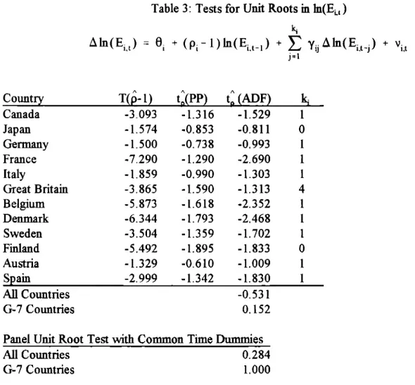
Tables 3 and 4 contain the redts of the unit root tests for nominal exchange rates and the PPP exchange rates, respectively. There is no evidence againm the null of a unit root for either of
the series, both when we consider each country individually and when we use the panel to carry our joint tests. In addition, in no instance do we fid evidence of determini~ic trends at the 5 percent level and in only one instance for each series do we find evidence at the 10 percent level, We therefore proceed assuming that both the nominal exchange rate and the PPP exchange rate for all countries in our panel contain a stochastic trend but no deterministic trend. Now that the preliminary testing is completed, we turn to the hypotheses of interest,
4.1 Relative Prices and Relat ive productivities
We be~ with the h~othesis that, in the long run, the relative price ofnontraded goods reflects relative productivities in the traded and nontraded goods sectors. Table 5 contains the redts of tests of the null hypothesis that the relative prices and the relative productivities are not cointegrated. The tests using data from an individual country yield mixed evidence. me
augmented Dickey-Fuller tests reject the null hypothesis of no cointegration for 7 of the 13 countries at the 10 percent leve~ and 6 of these 7 test statistics are also significant at the 5 percent level. The other NO tests provide less evidence against the n~. The results of the panel tests provide strong evidence that relative prices and relative producttities are, in fact, cointegrated. We reject the nd of no cointegration at the 5 percent level with all three tests, but when common time dummies are inckded only the t-tests yield rejections.
Because there is some evidence that deterministic trends might be in the data for some of the countries, we also carry out the panel corntegration tests rncluding a time trend in the
cointegrating regression. The evidence from these tests is not as strong, but, because only some of the series may have deterministic trends and because the critical values with deterministic trends are higher than those without deterministic trends, the tests are probably overly
consewative. The evidence is weake~ when we include common time dummies. When we exclude the 3 countries (Canada, Great Britain, and Austria) for which the data may not fit the stochastic assumptions that the test rely on, we reject at the 5% level for one of the three tests.
We conclude from table 5 that the relative prices of nontraded goods and the relative productivities in the traded and nontraded goods sectors are cointegrated as the Balassa-Samuelson model predicts. In tables 6 and 7 we turn to the stronger predictions of the Balassa-Samuelson model that the slope in the cointegrating relationship is 1.0. In table 6 we test this implication of the model by testing the nd hypothesis that there is a unit root in the ~erence between the (log) relative price and the (log) relative productivities, Once again the evidence is mixed when we look at the tests carried out on the data for each country individually. We reject the null hypothesis of a unit root in the difference at the 5 percent level for 5 of the 13 countries and at the 10 percent level for one additional country. Once again, however, the gain in power from using joint tests in a panel is clear. We reject the n~ hypothesis of a unit root at the 5 percent level for all three groups of countries that we consider. The evidence horn the tests without a time trend is clearly consistent with the hWothesis that the slope of the cointegrating relationship is 1.0, or, alternatively, that the relative price of nontraded goods is proportional to the relative productivities in the traded and nontraded goods sectors.
Inckding a time trend again weakens the evidence against the nd hypothesis of a unit root. When time common dummies are included, we reject the nd hypothesis of a unit root in the difference ordy when we consider all countries together. There are several interpretations for this haling. It maybe that the tests are overly consemative because ordy some of the series may have deterministic trends. It maybe that relative prices and relative productivities are
proportional in the long run for ordy some of the countries. Or it may be that the added power from using the fi.dl sample is responsible for the rejection when the fi.dl set of coutries is used.
The evidence in table 6 is generally consistent with the long run proportionality of relative prices and relative productivities. An altemat~e means of testing whether the slope of the cointegrating relationship is equal to 1,0 is to estimate the slope directly and do a t-test on the estimated slope. We report the redts of these tests in table 7. With three exceptions, Canada, Denmark, and Sweden, the slope coefficients are generally close to 1,0. The average My motied OLS slope estimate is roughly 0.8, and excluding the three countries with the slope around 0.5, the average is nearly 0.9. The slopes are fairly precisely estimated, however, and we can reject the null hypothesis that the slope is 1.0 at the 5 percent level for 9 of the 13 countries. The panel tests cob these results. When we include common time dummies we obtain at-ratio for the null that ~ = 1.0 of around -8.0 when we use all of the countries in the sample or when we exckde the three countries for which the series are most likely to violate the
assumptions about the stochastic trends,
The results of the formal tests are reflected in figure 2 where we plot the (log of the) relative price of nontraded goods and the (log of the) relative labor produtiivities in traded and nontraded goods for four countries, Germany, Japan, It sly, and the United States. The two series are normalized so that 1970 = O for each country, The ~erences between the two series
generally appear to be transitory although the data for the United States and Italy exhibit a tendency common to many of the countries we examine for the relative productivities to grow by more than the relative price. This tendency is reflected in the slope estimates, which are generally less than one.
4.2Mne ~s
Tables 6 and 7 contain contradictory results. The redts in table 6 are consistat tith a slope of 1.0 while the retit from table 7 are not, One possible explanation for the difference is the small sample properties of the my modi6ed OLS estimators. Phillips and Hansen ( 1990) fid that the FMOLS estimates can exhibit considerable small sample bias when e and ~ (born (12)) are persistent and when they are highly correlated. In order to explore whether small sample problems might be responsible for the ~erences between the results in tables 6 and 7, we conduct a series of Monte Carlo experiments. First we ve@ that the FMOLS estimates perform well even in samples of 25 observations when ~ and ~ are independent and identically distributed. Then we choose three countries: one (the United States) with a slope estimate of around 0.9, one (Belgium) with a slope estimate of around 0.8, and one (Denmark) with a slope estimate around 0.6. For each of the countries we estimate a VAR for q=(~, ()’ and use the parameters and error covanance matrix to generate 15,000 samples of 25 observations in which the true value of ~ is set to 1.0. We also examine the small sample properties of the pooled tests statistics from the corresponding 1,000 samples of 15 countries and 25 observations.
In all three cases we fmd that the FMOLS estimate of the slope is biased and that using the asymptotic distribution wodd lead to rejecting the null hypothesis of ~= 1.0 too frequently. The mean FMOLS estimates of ~ are: 0.90 when we use the U.S. parameters, 0.77 when we use the Belgian parameters, and 0.86 when we use the Danish parameters. Thus for two of the three we find that our point estimate from table 7 is roughly equal to the mean vake estimated from the Monte Carlos in which the true value of ~ is unity. The point estimate in table 7 computed from the Danish data (O.54) is below the average for the third and is significantly different from 1.0 at
the 5 percent level even using the empirical distribution from the Monte Carlo experiments.
The tendency for the FMOLS estimates to reject the nd of ~ = 1.0 too frequently and the downward bias in the estimate of ~ is also reflected in the panel test statistics. As is the case with the individual country tests, the panel tests (especidy the group mean test) reject too frequently. When the U, S. parameters are used to generate the data and all countries are used, the 95 percent critical value from the Monte Carlos is below the value reported m table 7 for all countries. The critical values computed from the Monte Carlos using the other two sets of parameters all exceed the test statistics reported in table 7.
The Monte Carlo evidence suggest that one wotid tend to Iind slope estimates below 1,0 (relative productivity changes outstripping relative price changes) even if the true slope was, in fact, 1.0. Thus the test statistics reported in table 7 should probably not be taken as evidence against the nti h~othesis that ~ is one. 12
Figure 2, the redts in tables 5, 6 and 7, and the Monte Carlo experiments taken together lend support to the first part of the Balassa-Samuelson hypothesis. The relative prices of
nontraded goods and the relative productivities in the traded and nontraded goods sectors appear to be cointegrated and the slope of the corntegrating relationship is close to 1.0 as the hypothesis predicts. Thus relative prices and relative productivities appear to be proportional in the long run
43h” P
~v Do ar N rair
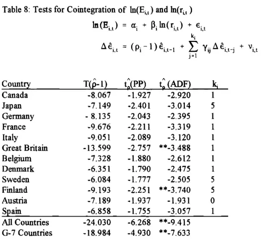
Next we turn to testing long run purchasing power parity in traded goods using the U. S. dollar as the numeraire currency. Table 8 presents the results of tests of the hypothesis that the
12Pedroni ( 1996) presents more extensive evidence on the small sample properties of the panel test statistics.
nominal exchange rate and the PPP exchange rate are not cointegrated, The tests earned out on the data from each individual country yield little evidence against the nu~ of no cointegration. The ADF tests reject the null at the 5 percent level for only two countries, Great Britain and Finland. We fmd no rejections tith either of the other NO tests. The benefit of pooling the data in the panel tests is, once again, clearly apparent. The panel tests provide evidence that the nominal and PPP exchange rates are cointegrated. When we include common time dummies, au three test rejects the nd of no cointegration at the 5 percent level.
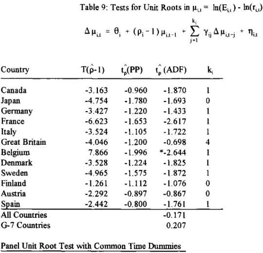
The redts in table 8 suggest that nominal exchange rates and PPP exchange rates are probably cointegrated when the U.S. dollar is the numeraire currency. If purchasing power parity holds for traded goods, they shodd be cointegrated with a cointegrating slope of 1.0. Next we test this stronger restriction of purchasing power parity and report the results in tables 9 and 10. If purchasing power parity holds in the long run for traded goods, the ~erence between the nominal exchange rate and the PPP exchange rate should be stationary. In table 9 we report the results of tests of the nti hypothesis that there is a tit root in the difference. The tests using the data from each country individually provide no evidence against the nd hypothesis of a unit root. The panel test points to a rejection of the null h~othesis when common time dummies are used. 13 Otherwise the panel test yield no evidence against the nd. Athough nominal exchange rates and PPP exchange rates are cointegrated, the ~erence between them appears to be nonstationary.
13This rejection might appear surprising given the tiihue to reject the null of no cointegration on the nominal and PPP exchange rates with the other tests. The reason for this rejection becomes clearer in the next section when we change numeraire currencies. Because changing the numeraire amounts to adding the same log exchange rate to each cross-sectional unit, it ti have no impact on tests computed usrng deviations from cross-section means, at least for large N. As can be seen by comparing the resldts in tables 8 and 12, with N= 12, a change of nmeraire retits in ody minimal changes to the test statistics. See O’Connell ( 1996).
Contrary to the predictions of purchasing power parity in traded goods, the slope of the cointegrating relationship appears not to be 1.0.
In table 10 we present estimates of the slopes of the cointegrating relationships along with tests of the hypothesis that the slope is 1.0. Consistent with the results in table 9, we find that we reject the null hypothesis that the slope is 1.0 for 10 of the 12 countries and the panel test strongly reject the null hypothesis that the slopes are jointly equal to one. We also found a large number of rejections of the null when we looked at the cointegrating slopes for relative prices and relative productivities, but the reason for the large number of rejections is quite ~erent here. There the rejections arise because the slope estimates, which are fairly close to 1,0, are precisely estimated. In contrast, here the point estimates are all far from 1.0 and we reject the nfl despite fairly large standard errors. The wide range of point estimates that we report in table 10 is roughly consistent with previous work that has looked at purchasing power parity. In their survey, Froot and Rogoff (1995) repoti that it is common in the literature to find slopes that vary widely across countries and are frequently far from the value of 1.0 that is implied by purchasing power parity.
4.4 Pure hasinz Power Paritv in Traded Goods :DMast he Numeraire Currency
Do the results on purchasing power parity in traded goods depend on the choice of the U, S. dollar as the numeraire currency?14 In order to shed some light on this question, we now reconsider our tests using the DM as the numeraire currency. In table 11 we present the redts of
‘4Two pieces of existing evidence suggest that it might. Papell ( 1995) tests the null hypothesis of a unit root in real exchange rates computed with consumer prices and fids stronger rejections when the DM is used as the reference currency than when the dollar is used as the reference currency. Similarly, Jorion and Sweeney (1994) find stronger evidence that real exchange rates are mean reverting when the DM is used as the numeraire. On the other hand, Wei and Parsley ( 1995) use prices in 12 tradable sectors and fmd that rates of convergence to purchasing power parity are similar when the DM and the U, S. dollar are used as the numeraire.
tests of the nti hypothesis that nominal exchange rates and PPP exchange rates are not
cointegrated.’s The tests carried out on individual country data reject the null hypothesis only for the three Scandinavian countries. The results of the joint tests are somewhat stiar to those found using the U.S. dollar as the numeraire. The added power derived from using a panel is again apparent and the nd of no cointegration is strongly rejected.
The results in table 11 suggest that nominal and PPP exchange rates relative to the DM (like those relative to the dollar) are cointegrated, Next we turn to tests of the prediction that the cointegrating slope coefficient is one. Again, the fist test inrposes the null hypothesis that the slope is 1.0 and examines whether the ~erence between nominal and PPP exchange rates is stationary. We present the results of these unit root tests in Table 12 and find fairly strong evidence against the nti hypothesis of a unit root in the difference, We reject the null hypothesis with at least two of the three tests for five of the twelve countries taken individually and with one of the tests for a sixth country. The joint tests yield rejections at the 95°/0 level or greater.
Next we estimate the cointegrating slope and report the results in table 13. These resuks provide an interesting contrast to those obtained using the U. S. dollar as the numeraire currency, Although we reject the null hypothesis that the slope is 1.0 for tie of the twelve currencies, the point estimates are fairly close to 1.0, and are much closer to 1.0 than are those obtained with a
15We also test for unit roots in nominal exchange rates and PPP exchange rates (both relative to the DM) but do not report the results. We find no evidence against the null of a unit root in nominal exchange rates and only for Belgium do we fid strong evidence against the null of a unit root in PPP exchange rates. We also reject the m.dl of a unit root in the PPP exchange rates for Sweden and Austria using one of the three tests. Finafly, we do not tid deterministic trends in either the nominal or PPP exchange rates.
dollar numeraire. ‘b the point estimates
Even for the cmencies for which we reject the null hypothesis of a unit slope, are closer to one than are any of the slopes we obtain using the dollar as the numeraire,
The results we report in tables 11-13 lend somewhat favorable support for the h~othetis of purchasing power parity in traded goods when the DM is the numeraire currency. Nominal exchange rates and PPP exchange rates appear to be cointegrated and, although we can fiequentb reject that the two are proportional in the long run, our estimates suggest that they are nearly proportional for the currencies we consider. Interestin@y, the evidence does not indicate that purchasing power parity in traded goods is any more likely to hold for European currencies than
for non-European currencies relative to the DM.
h figure 3 we plot the (logs of the) nominal and PPP exchange rates for the DM and yen relative to the U, S. dollar and the lira and yen relative to the DM. Agarn, each series is
normalized so that 1970 = O. Large and long-lasting deviations from PPP m traded goods are evident for both exchange rates relative to the U.S. dollar. As is consistent with the formal tests, these deviations are smaller and less persistent when we examine the two exchange rates relative to the DM.
5. Concluti~ Remarks
How well does the Balassa-Samuelson model explain the behavior of real exchange rates?
16me one notable exception is the Belgian franc regression where we obtain a negative point estimate and a large standard error. Recall that we rejected the m.dl hypothesis of a unit root in the Belgian franc - DM PPP exchange rate but not for the nominal exchange rate. The two therefore cannot be cointegrated so that the estimate is not particularly bothersome. The slope for the U.S. dollar - DM exchange rate is, of course, identical to that reported in table 10.
The evidence from a panel of 13 OECD countries supports the h~othesis that the relative price ofnontraded goods reflects the relative labor productivities in the traded and nontraded goods sectors. The results suggest that the relative prices of nontraded goods and the relative
productivities in the traded and nontraded goods sectors are corntegrated and that the slope of the cointegrating relationship is generally close to 1.0. For some comtries, groti m relative
productivities appears to outstrip growth in relative prices (or equivalently the slope is less than 1.0), but Monte Carlo evidence suggests that this tierence is within the range of sampling variation in a sample like ours. Thus relative prices and relative produtities appear to be proportional in the long run.
But the Balassa-Samuelson model also assumes that traded goods prices are characterized by purchasing power parity. As is consistent with the evidence presented in Engel ( 1995), we find large and long-wed deviations from PPP in traded goods when we look at U.S. dollar exchange rates. Although nominal exchange rates and PPP exchange rates appear to be cointegrated we fid that the slopes of the cointegrating regressions differ vary widely and ~er substantially from one. But when we examine DM exchange rates the evidence is considerably more favorable to purchasing power parity in traded goods. Nominal and PPP exchange rates appear to be cointegrated and the slopes of the cointegrating regressions are much closer to one than is the case with U.S. dollar exchange rates. This evidence suggests that Engel’s results may well be sensitive to the choice of numeraire currency. hterestin~, apart from the U.S. dollar - DM exchange rates, purchasing power parity does not appear to be a better characterization of DM exchange rates rebtive to European currencies than relative to non-European currencies.
Referaces
Asea, Patrick K and Enrique G. Mendoza ( 1994), “The Balassa-Samuelson Model: A General Equilibrium Appraisa~” Review of International Economics 2, pp. 244-267.
Asea, Patrick K and Max Corden ( 1994), “The Bakssa-Samuelson Model: An Overview,” Review of Internat ional Econom ‘C$2, pp.
Balassa, Bela ( 1964), “The Purchasing Power Parity Doctrine: A Reappraisa~” Journal of Political Economy 72, pp. 584-596.
Chinn, Menzie David ( 1995), ‘Whither the Yen? Implications of an Intertemporal Model of the Yen.iDollar Rate,” working paper, Department of Economics, University of California, Santa C- October 1995.
Chinn, Menzie David, and Louis Johnston ( 1996), “Real Exchange Rate levels, Productivity and Demand Shocks: Evidence from a Panel of 14 Countries,” working paper, Department of Economics, University of CaMornia, Santa C~ January 1996.
De Gregorio, Jose, Alberto Giov- and Thomas Krueger ( 1993), “The Behavior of
Nontradable Goods Prices in Europe: Evidence and Interpretation,” working paper, International Monetary Fund, April 1993.
De Gregorio, Jose, Alberto Giovd and Holger Wolf( 1993), “International Evidence on Tradables and Nontradables Inflation,” working paper, International Monetary Fund, September
1993,
Dickey, David A And Wayne A. Fuller (1979), ‘~stribution of the Esttitors for
Autoregressive Time Series with a Unit Root,” Journal of the American Stat istical Association 74, pp. 427-431.
Enge~ Robert F. and Clive W. J. Granger ( 1987), “Co-rntegration and Error Correction: Representation, Estimation, and Testing,” Econometn “C~55, pp. 251-276.
Engle, Charles ( 1995), “Accounting for U. S. Real Exchange Rate Changes,” NBER working paper no. 5394, December 1995.
Evans, Charles (1992), ‘Productivity Shocks and Real Business Cycles,” Jouma 1 of Monetan EconomiC~ 29, pp. 191-208.
Froot, Kenne@ andKermethRogoff(1991), ‘me EMS, the EMU and the Transition to a
Common Currency,” NBER Macroeconomics Annual 6, pp. 269-317.
Froot, Kemeth, and Kenneth Rogoff ( 1995), ‘Perspectives on PPP and Long-Run Real Exchange Rates,” in Gene Grossman and Kenneth Rogoff (eds. ) Handb ook of International Economics, Volume 3, North Holland.
Hal AlaStair ( 1994), “Testing for a Unit Root in Time Series with Pretest Data-Based Model Selection,” .loumal of Business and Economic Statistic$ 12, pp. 461-470.
~ K~gso, M. Hashem Pesaran, and Yongcheol Shin (1995), “Testing for Unit Roots in Heterogeneous Panels,” working paper, Department of Applied Economics, University of Cambridge, June 1995.
Jorion, Philippe and Richard D. Sweeney ( 1994), ‘Mean Reversion in Real Exchange Rates: Evidence and @lications for Forecasting,” working paper, Georgetown University.
Marston, Richard ( 1987), “Real Exchange Rates and Productivity Growth in the United States and Japan,” in Arndt, Sven and J. David Richardson (eds), Real-Financ ial Linkages amohg Ouen Economies, MIT Press, 1987.
Mankiw, Gregory ( 1989), ‘Real Business Cycles: A New Keynesian Perspective,” Journal of Eco nomic Persoe ctives 3 pp, 79-90.
Newey, Whitney K And Kenneth D. West (1994), “Automatic Lag Selection in Covariance Matrix Estimation,” Review of Economic Stuch“es 61, pp. 631-653.
Ng, Serena and Pierre Perron ( 1995), “Unit Root Tests in ARMA Models with Data-Dependent Methods for the Selection of the Truncation Lag,” Jouma 1 of the American Statistical Association 90, pp.268-281.
O’Conne~ Paul ( 1996), ‘me OverValuation of Purchasing Power Parity,” working paper, Harvard University, April 1996.
Pape~ David H, (1995), “Searching for Stationarity: Purchasing Power Parity Under the Current Float,” working paper, Department of Economics, University of Houston, October 1995.
Pedro~ Peter ( 1995), “Panel Cointegration: Asymptotic and Finite Sample Properties of Pooled Time Series Tests with and Application to the PPP Hypothesis,” working paper, Department of Economics, Indiana University, June 1995.
Pedro~ Peter ( 1996), ‘Tully Motied OLS for Heterogeneous Panels,” working paper, Department of Economics, Indiana University, March 1996.
Phillips, Peter C.B. and Bruce E, Hansen ( 1990), “Statistical Inference in hstrumental Variables Regressions with 1(1) Processes,” Review of Economic Stud “es 57, pp. 99-125,
Phillips, Peter C.B. and Sam Ouliaris ( 1990), “Asymptotic Properties of Residual Based Tests for Cointegration,” Econometric 58, pp. 165-193,
Phillips, Peter C. B. and Pierre Perron ( 1988), ‘Testing for a Unit Root in Time Series Regression,” Biometrik~ 75, pp. 335-346.
Samuelson, Pad ( 1964), “Theoretical Notes on Trade Problems,” Review of Economics and ~ 46, pp. 145-154.
Summers, Lawrence (1986), “Some Skeptical Observations on Real Business Cycle Theory,” Federal Reserve Bank of Minneapolis @arte rlv Review 10, pp. 23-27.
-WeL Shang-Jin and David C. Parsley (1995), “Purchasing Power Dis-Parity During the Floating Rate Period: Exchange Rate Volatility, Trade Barriers, and Other Culprits,” working paper, Kennedy School of Government, March 1995,
Appendix: THE DATA
Nominal exchange rates are from International Financial Statistics. Sectoral price and productivity data for Belgi~ Canada, Denmark, Great Britain, Firdand, France, Germany, Italy, Japan, Sweden, and the US come from the OECD National Accounts. Price and productivity data for Austria and Spain come from national statistics. (Francisco de Castro of the Bank of Spain coflected and documented the data, ) These sources provide annual sectoral data on
nominal value added, real value added and number of employees. The traded sector is made up of the “manufacturing” sector and the “agricdture, hunting forestry and fishing” sector. The non-traded sector is made up of the “wholesale and retail trade, restaurants and hotels” sector, the “trmsport, storage and commtication” sector, the “finance, insurance, real estate and business setices” sector, the “community social and personal services” sector, and the “non-market services” sector; the “non-market services” sector is made up of the “producers of government services” subsector and the “other producers” subsector.
Data consistency is always an issue, We are aware of the foflowing anomahes in the OECD data: (1) The German market services emplo~mt figures do not include the “real estate and business services” sector; value added figures do. (2) The Italian, British and Belgian value added and emplo~ent figures do not include “real estate and busrness services” sector. (3) BritiA value added and employmmt figures consist of the “producers of government setices” sector; they do not rnclude the “other producers” sector.
Table 1: Tests for Unit Roots in ln(~, )
ki
A~(qiL) D Oi + (pi- l)~(qi,t. [) + ~ yij A~(qi,L-j) + ‘it j=l
country T(fi-1) t:(PP) t: (ADF) ~
United States 0.558 0.829 0.801 0 Canada -7.023 -1.669 -0.942 2 Japan -0.785 -1.478 -1.410 0 Germany -1.931 **-3.116 -2.515 1 France -1.180 -1.408 -1.345 4 Italy 0.587 1.220 1.166 0 Great Britain -2.234 -0.949 -1.757 1 Belgium -1.326 -2.406 -2.283 0 Denmark -2.760 **-3.992 **-4.178 3 Sweden -0.096 -0.043 -0.041 0 Finland 1.919 0.847 0.986 2 Austria -0,683 -1.321 -1.259 0 Spain -1,897 -1.264 -0.563 4 All Countries 1.858 G-7 Countries 1.836
Panel Unit Root Test with Common Time Dummies
All Countries 0.060
G-7 Countries 0.064
Joint Tests of Unit Roots Allowing for Deterministic Trends
All Countries -0.808
G-7 Countries -0.746
Panel Unit Root Test with Trends and Common Time Dummies
AU Countries 1.587
G-7 Countries 1.020
Notes: Statistical si~cance at the 95% level or greate{ is signified by **. Significance at the 90% level or greater is siguified by *, The T(6- 1) and tP(PP) statistics are ~ests proposed by Phillips and Perron and are computed from re~essions setting ~=0. The tP(ADF) is the augmented Dickey-Fuller statistic. The jornt tests are the panel unit root tests proposed by @ Peseran, and Shin ( 1995) and are distributed as standard normal.
Table 2: Tests for Unit Roots in ln(~, / %, )
ki
Aln(xi(/ni,,, ) = ei + (pi -1 ) ~(xi~/ni,t) + ~ YijA~(xl,t/ni,l) + ‘i,t j=~ country T(~-1) t:(PP) t: (ADF) ~ United States 0.476 0.717 0.692 0 Canada -1.499 -0.829 0.248 3 Japan **.13 222 **.3,360 **-3.161 3 Germany -2:017 -2.482 -2.400 0 France -0.469 -0.922 -1.061 2 Italy -0.061 -0.123 -0.883 3 Great Britain -2.263 -1.555 -1.476 0 Belgium -0.600 -1.327 -1.259 0 Denmark -2.705 -2.500 -2.402 0 Sweden -0,290 -0.274 0.283 4 Finland 1,496 0.760 0.735 0 Austria 0,327 1.045 1.867 4 Spain -0.569 -1.184 -1,647 4 All Countries 3.574 G-7 Countries 2.441
Panel Unit Root Test wifi Common Time Dummies
All Countries -1.304
G-7 Countries -0.430
Joint Tests of Unit Roots Allowing for Deterministic Trends
All Countries 0.484
G-7 Countries 0.131
Panel Unit Root Test with Trends and Common Time Dummies
All Countries -0.841
G-7 Countries -1.603
Notes: Statistical significance at the 9570 level or greater is signified by **. Significance at the 90% level or greater is si@ed by *. The T(~- 1) and t~(PP) statistics are ~e~s proposed by Phillips and Perron and are computed from recessions setting ~=0. The tP(ADF) is the augmented Dickey-Fder statistic. The joint tests are the panel unit root tests proposed by ~ Peseran, and Shin ( 1995) and are distributed as standard normal.
Table 3: Tests for Unit Roots m In(EL,) 4
A~(Eit)
=
Oi +
(~i-l)~(Ei.t.l)
+ ~
yij
A~(Ei,t-j)+
Vi,t
j=l
country T(J- 1) t:(PP) t:(ADF) &
Canada -3.093 -1.316 -1.529 1 Japan -1.574 -0.853 -0.811 0 Germany -1.500 -0.738 -0,993 1 France -7,290 -1.290 -2.690 1 Italy -1.859 -0.990 -1.303 1 Great Britain -3.865 -1.590 -1.313 4 Belgium -5.873 -1.618 -2.352 1 Denmark -6.344 -1.793 -2,468 1 Sweden -3,504 -1.359 -1,702 1 Ftiand -5.492 -1.895 -1.833 0 Austria -1.329 -0.610 -1.009 1 S~ain -2.999 -1.342 -1.830 1 M Countries -0.531 G-7 Countries 0,152
Panel Unit Root Test with Common Time Dummies
All Countries 0.284
G-7 Countries 1.000
Joint Tests of Unit Roots Allowing for Deterministic Trends
All Countries -2.335
G-7 Countries -1,628
Panel Unit Root Test tith Trends and Common Time Dummies
AU Countries 0.635
G-7 Countries -1.187
Notes: Statistical significance at the 95% leve\or ~eate~ is signified by **. Significance at the 90V0 level or greater is signified by *. The T(p- 1) and tP(PP) statistics are ~ests proposed by Phillips and Perron and are computed horn regressions setting ~=0. The tP(ADF) is the augmented Dickey-F~er ~atistic, The joint tests are the panel unit root tests proposed by k Peseran, and Sti ( 1995) and are distributed as standard normal.
Table 4: Tests for Unit Roots in In(rL,) h
A~(ri,,) =
ei +
(pi- l)~(ri,t)
+ ~ yij A~(ri L) +
Vit
j=l country T(~-1) t:(PP) t: (ADF) ~ Canada -0.310 -0.215 0.091 2 Japan -0.061 -0.037 0.42 0 Ge~y -2.210 -1.022 -1.325 1 France 0.192 0.159 -0.423 0 Italy 0.193 0,275 -0.175 2 Great Britain 0.102 0.110 -0.201 1 Belgium -2.140 -0.971 -0.797 0 Denmark -0.497 -0.542 -0.520 0 Sweden -0.342 -0.382 -0.274 0 Finland -1.094 -1.503 -1.353 2 Austria -2.227 -0,988 -1.583 2 Spain 0.280 0.438 -0.265 1 AU Countries 3.566 G-7 Countries 3.177Panel Unit Root Test with Common Time Dummies
All Countries 0.475
G-7 Countries 1.939
Joint Tests of Unit Roots Allotig for Deterministic Trends
All Countries -0.425
G-7 Countries -0.010
Panel Unit Root Test with Trends and Common Time Dummies
All Countries -1.065
G-7 Countries 1.037
Notes: Statistical significance at the 95% level or greater is sigui.tied by **. Si@cance at the 90% level or greater is signified by*. The T(fi- 1) and t~(PP) statistics are ~ests proposed by Phillips and Perron and are computed from recessions settrng ~=0. The tP(ADF) is the augmented Dickey-F~er statistic. The jornt tests are the panel ti root tests proposed by m Peseran, and Shin ( 1995) and are distributed as standard normal.
Table 5: Tests for Cointegration of ln(~t ) and In(<t / ~, ) h(qit) = ai + pi ln(xiL/ni,t) + Eit
ki ‘
‘ei~ = (Pi- l)ei~-, + X Yij Aei,t-j + ‘i,t j=l country T(~-1) t;(PP) t; (ADF) k United States Canada Japan Germany France Italy Great Britain Belgium Denmark Sweden Finland Austria sDain *-18.106 -11.921 -8.643 -16.084 -8.976 -5.798 -8.277 -12.641 -6.546 -6.851 *-18.637 -11.208 -9.809 **-3.483 -2.856 -3.052 *-3.200 -2.425 -1.650 -2.029 *-3. 184 -1.894 -1.867 **-3.590 *-3. 172 -2.494 *“*-3.367 **-5.446 **-3.521 **-3.946 -2.642 -2,949 -1.732 -3.025 -1.762 **-4.539 **-5.593 -3.021 *-3.356 4 2 3 3 3 3 0 0 2 5 1 0 3 All Countries **-33.906 **-9.421 **-14.606 No C& ~ AU **.29.077 **-8.172 **-13,636 G-7 Countries **.24,841 **.7.220 **-11.621 Panel Tests of Cointegration with Time ~es
All Countries -23.707 -7,494 **-8,889 No CA ~ AU -18.177 **-7,811 **-9.881 G-7 Countries -14.457 **-7.074 **-7.586
Joint Tests of Cornte~ation Allowing for Dete_ic Trends All Countries -36.935 -9.235 **-12.132
No C& ~ AU -33.096 -8.261 **-10.981 G-7 Countries -25.684 -6.614 **-8.488
Panel Tests of Cointegration with Trends and Time Dummies All Countries -31.293 -7.820 -8.996
No CA ~ AU -32.994 -8.306 **-10,878 G-7 Countries -25.380 -5.914 -7.214
Note!: Signi6cance at the 95% and 90% levels are noted by ** and **, respective~. The T(6- 1) and tP(PP) statistics are Phillips-Perron tests applied to the residuals from the first re~ession and are computed with ~=0. The t~(ADF) is the augmented Dickey-Fder statistic. Cfiical values are taken from the tables compiled by P-s and Ouliaris (1990). The panel corntegration tests
country T(fi-1) t;(PP) t; (ADF) ~ United States -9.458 -2,367 -2.287 0 Canada -6.858 -2.437 -2.312 0 Japan -7.996 **-3,307 **-4.21O 3 Germany **-15.327 **-3.075 **-3.208 1 France -4.100 -1.411 -0.451 2 Italy -4.938 -1,775 **-3.060 3 Great Britain -6.467 -2.139 -2.030 0 Belgium 0.046 0.026 1.238 5 Denmark -2,850 -1.650 -1.540 0 Sweden -6.361 -2.079 -2.292 1 Finland **.21.268 **-3.311 **-5.322 1 Austria *-10.391 *-2.841 *-2.709 O spain -8,053 -2.100 **-3.819 3 All Countries **-3,721
Excluding Canada, Great Britain, Austria **-3.473
G-7 Countries **-2.638
Panel Unit Root Test with Common Time Dummies
AU Countries **-4. 114
Excluding Canada, Great Britarn, Austria **-3.703
G-7 Countries **-2.040
Joint Tests of Unit Roots Allowing for Dete-ic Trends
AU Countries ** -4.164
Excluding Canada, Great Brit@ Austria **-4.261
G-7 Countries **-3.281
Panel Unit Root Test with Trends and Common Time Dummies
AJl Countries **-1.977
Excluding Canada, Great Bnt~ Austria -0.403
G-7 Countries -0,512
Notes: Si@cance at the 95% and 90V0 levels is noted by ** and*, respectfie~. The T(c- 1) ~d t~(PP) statistics are tests proposed by Pus and Perron and are computed setting ~=0. The tP(ADF) is the augmented Dickey-Ftier statistic. The jornt tests are the panel unit root tests proposed by h Peseran, and Shin ( 1995) and are distributed as standard normal.
Table 7: Estimates of the Cointegrating Slope Coefficient of ln(~, ) ~d h(<t / ~, )
‘(qi,t) =
ai + Pi‘(xi.~jni,l)+
‘1,1
country~o, s t(p~”l) No. Lags
United States 0.887 0.887 **-3.852 3 Canada 0.455 0.442 **-6.243 2 Japan 1.045 1.006 0.092 2 Germany 1.050 1.037 1.013 2 France 0.771 0.755 **-3.791 2 Italy 0.883 0.892 **-2.007 2 Great Britarn 0.700 0.728 **-2.082 2 Belgium 0,791 0.785 **-8.369 2 Denmark 0.544 0.512 **-10. O29 1 Sweden 0.574 0.537 **-3.929 2 Finland 0.956 0.909 -1.455 5 Austria 0.959 0.929 -1.398 2 Spain 0.895 0.859 **-2. 141 3
Panel Tests of@ = 1
t; @;
All Countries **-10.295 **-12.256
Excluding CA ~ AU **-9.865 **-10.899
G-7 Countries **-5.203 **-6.376
Panel Tests of ~ = 1 with Common Time Dummies
t; @i
All Co~tries **-8.318 **-7,866
Excluding CA ~ AU **-7. 107 **-8.917
G-7 Countries **-3.086 **-2.296
Notes: The second column contains the ordinary least squares estimates of the slope coefficient. Column 3 contains the Phillips-Hansen ( 1990) fi.dly mowed OLS estimates of the slope and column 4 contains the t-ratio formed by subtracting one from the fully modified OLS estimate of the slope and dividing by the corresponding standard error. The number of lags used in
computing the My modified OLS estimate and its standard error is reported in cob 5 and are chosen using the data dependent procedure proposed by Newey and West (1994). The panel tests are those proposed by Pedroni ( 1996),
Table 8: Tests for Cointegration of h(Ei, ) and In(rL,) h(Ei,) = ai + ~iln(ri,,) + ~i,
4’
A~i,t = (pi- l)~i,t-l + ~ yij Agit-j + Vit j=l country T(~-1) t:(PP) t; (ADF) k Canada Japan Germany France Italy Great Britain Bel@um Denmark Sweden Finland Austria -8.067 -7.149 -8.135 -9.676 -9.051 -13.599 -7.328 -6.351 -6.084 -9.193 -7.189 -1.927 -2.401 -2.043 -2,211 -2.089 -2.757 -1.880 -1.790 -1.777 -2.251 -1.937 -2.920 -3,014 -2.395 -3,319 -3.120 **-3.488 -2.612 -2.475 -2.505 **-3.740 -1,931 1 5 1 1 1 1 1 1 5 5 0 Sparn -6.858 -1.755 -3.057 1 All Countries -24.030 -6.268 **-9.415 G-7 Countries -18.984 -4.930 **-7.633 Panel Tests of Cointe~ation ~ Time Dummies All Countries **.33.515 **-8.495 **-9.696 G-7 Countries **-26.054 *.5.956 **-6.759
Notes: Statistical si@cance at the 95V0 leve~or greate~ is si@ed by **. Si@cance at the 90% level or greater is signi.tied by *. The T(p- 1) and tP(PP) statistics are Phillips and Perron tests applied to the residuals from th~ fist regression and are computed from re~essions setting ~=0 in the second regression. The tP(ADF) is the augmented Dickey-Fuller statistic.
Significance levels for these tests are taken from the tables compiled by P~s and Waris (1990). The jornt tests are the panel cornte~ation tests proposed by Pedroni (1995). Si@cance levels for these te~s are computed from tables compiled by Pedroni.
Table 9: Tests for Unit Roots in pit = ln(EL,) - In(rL,)
ki
A ~it z ei + (pi -1 ) ~it.l + ~ Yij A~i,t-j + ~i,t j=l
country T(;- 1) t;(PP) t; (ADF) &
Canada -3.163 -0.960 -1.870 1 Japan -4.754 -1.780 -1.693 0 Germany -3.427 -1.220 -1.433 1 France -6.623 -1.653 -2.617 1 Italy -3.524 -1.105 -1.722 1 Great Britain -4.046 -1.200 -0.698 4 Belgium 7.866 -1.996 *-2.644 1 Denmark -3.528 -1.224 -1.825 1 Sweden -4.965 -1.575 -1.872 1 Finland -1.261 -1.112 -1.076 0 Austria -2.292 -0.897 -0.867 0 spain -2.442 -0,800 -1.761 1 All Countries -0.171 G-7 Countries 0.207
Panel Unit Root Test with Common Time Dummies
All Countries **-2.754
G-7 Couutries -0.651
Notes: Statistical si@cance at the 95% level or greater is signified by **, Significance at the 90% level or greater is signified by *. The T(6- 1) and t~(~P) statistics are tests proposed by Phillips and Perron and are co~uted setting ~=0. The tP(ADF) is the augmented Dickey-Fuller statistic, the t ratio. The jornt tests are the panel unit root tests proposed by ~ Peseran, and Shin (1995) and are distributed as standard normal.
Table 10: Estimates of the Cointegrating Slope Coefficient of In(EL,) and In(ri, ) h(Eilt) = ~i + ~i~(rit) + ‘i,t
country 0,01s OiFMOIS t(pw, “y=1) No. Lags
Canada 0.516 0.483 **-4.853 2 Japan 1.934 1.603 1.450 2 Germany 2.463 2.035 1.566 3 France 0.448 0.302 **-3.734 3 Italy 0.688 0.682 **-3.852 3 Great Britain 0.525 0.496 **-5.243 1 Belgium 0.543 0.103 **-2.247 3 Denmark 0.025 0.019 **-4. 164 3 Sweden 0.557 0.510 **-2.221 3 Ftid 0.264 0.264 **-6.994 3 Austria 2,670 2.235 **1.999 3 spain 0.596 0.562 **-3.395 3 Panel Tests of h = 1 t; fi; All Countries **-11.177 **-9. 184 G-7 Comtries **.7.459 **-5.987
Panel Tests of b = 1 with Common Time Dummies
t; @i
All Countries **-32.277 **-22.448
G-7 Countries **6.458 **6. 148
Notes: The second cob contarns the ordinary least squares estimates of the slope coefficient. Column 3 contains the PhillipsHansen ( 1990) ~ motied OLS estimates of the slope and column 4 contains the t-ratio formed by subtracting one from the ~ modified OLS estimate of the slope and dividing by the corresponding standard error. The number of lags used in
computrng the@ modified OLS estimate and its standard error is reported m cohmm 5 and are chosen using the data dependent procedure proposed by Newey and West (1994). The panel tests are those proposed by Pedroni (1996),
Table 11: Tests for Cointegration of ln(Ei, ) and ln(rL, ), DM Numeraire country T(~-1) t:(PP) t: (ADF) ~ United States -8.135 -2.043 -2.462 1 Canada -9.193 -2,303 -2.663 4 Japan -12.932 -2.886 -2.327 5 France -7.204 -2.285 -2.115 5 Italy -12.547 -2.768 -2.542 5 Great Britain -6.471 -2.073 -2.034 0 Belgium -0.474 -0.462 -0.789 3 Denmark **.21.346 **-5.183 **-4.296 4 Sweden *.18,432 **-3.871 **-5.933 1 Finland *.19,841 **.3.466 **.4.084 1 Austria -11.256 -2.902 -2.849 0 Spain -14.197 -2.983 -2.930 0 AU Countries -21.146 -7.146 **-8.663 European Countries **.31. 187 **.7.962 **-8.874 Panel Tests of Cointe~ation with Time Dummies AU Countries **.32,403 **-8.272 **-10.O18 European Countries **-33, 130 **-8.455 **-10.494
Notes: Stati~ical significance at the 95% level or greater is signified by **, Si@cance at the 90% level of greater is sigili.fied by *. The T(6- 1) and t~(PP) statistics are Pus and Perron tests applied to the residuals from the first regression and are computed from regressions setting &=O in the second regression. The t~(ADF) is the augmented Dickey-Ftier statistic.
Significance levels for these tests are taken from the tables cotupiled by Phillips and Ouliaris (1990). The jornt tess are the panel corntegration tests proposed by Pedroni (1995). Si@cance levels for these tests are computed from tables compiled by Pedroni.
Table 12: Tests for Unit Roots m pi, = ln(EL,) - ln(ri,), DM Nurneraire A~i,t n Oi + (pi-l)Pit-l + $ Y,jA ~i~-j + Ti,,
j=l country T(~-1) t;(PP) tj (ADF) ~ United States Canada Japan France Italy Great Britain Belgium Denmark Sweden Finland Austria sDain -3,427 -7.052 *-10.708 -4.027 -7.718 -6.255 -0.595 **-20.501 -10.110 *-11.470 *-10.843 **-14.185 -1.220 -1.890 *-2.676 -1,826 -2,221 -2.076 -0.475 **-4.304 **-3.043 *-2.669 *-2.862 **-3.016 -1.433 -2.190 -2.545 -1.766 -2.148 -2.008 -0.459 **-4. 128 -0.809 -1.391 *-2.769 *-2.902 1 1 0 0 0 0 0 0 3 3 0 0 All Countries **-2,000 European Countries *- 1,720
Panel Unit Root Test tith Common Time Dummies
All Countries **-2. 194
European **-2.872
Notes: Statistical significance at the 95% level or ~eate~ is si@ed by **. Si@cance at the 90V0 level of greater is signi6ed by *. The T(6- 1) and tP(~P) statistics are tests proposed by Phillips and Perron and are computed setting ~=0. me tP(ADF) is the au~ented Dickey-Fuller statistic, the t ratio. The jornt tests are tie panel unit root tests proposed by @ Peseran, and Shin (1995) and are distributed as standard normal.
Table 13: Estimates of the Cointegrating Slope Coefficient of h(EL, ) and In(rit ), DM Numeraire ln(Ei,) = ai + ~iln(ri,) + ~i,
count ~ t No. La s United States 2.463 2.030 1.559 3 Canada 1.454 1.313 1.831 3 Japan 1.311 1.088 0.376 2 France 1.351 1.264 2.928 4 Italy 1.101 1.072 2.907 4 Great Britain 1.075 0.984 -0,155 4 Belgium -1.064 -0.597 -0.689 4 Denmark 1.058 1.062 2.515 2 Sweden 1.154 1.168 5.107 4 Finland 0.873 0.857 -3.637 2 Austria 1.059 1.021 0.046 4 Spain 1.010 1.000 -0.015 2 Panel Tests of fi = 1 t: fii All Countries **3.360 **2.983 European Countries **2.780 **2. 174
Panel Tests of ~ = 1 with Common Time Dummies
t; fii
All Countries **-7.625 **-8.533
European Countries **-6.152 **-7.676
Notes: The second column contains the ordinary least squares estimates of the slope coefficient. Column 3 contains the PhiJJipsHansen ( 1990) My motied OLS estimates of the slope and coti 4 contains the t-ratio formed by subtracting one from the my motied OLS estimate of the slope and dividing by the corresponding standard error. The number of lags used in
conrputrng the @ modified OLS estimate and its standarderroris reported m column 5 and are chosen using the data dependent procedure proposed by Newey and West (1994). The panel tests are those proposed by Pedroni ( 1996).
,
000000 00
m* mm- N