A robust fuzzy mathematical programming model for the closed-loop supply chain network design and a whale optimization solution algorithm
Javid Ghahremani-Nahr† Ramez Kian‡∗ Ehsan Sabet††
†Academic Center for Education, Culture and Research (ACECR), Tabriz, Iran ‡ Nottingham Business School, Nottingham Trent University, Nottingham NG1 4FQ, UK
‡ Department of Industrial Engineering, University of Tabriz, Tabriz, Iran ††Wolfson School of Mechanical, Electrical and Manufacturing Engineering
Loughborough University, Leicestershire LE11 3TU, UK August 9, 2018
∗
Corresponding author. Tel.: +44 115 84 82939.
E-mail addresses: [email protected] (J. Ghahremani-Nahr), [email protected] (R. Kian), [email protected] (E.Sabet)
A robust fuzzy mathematical programming model for the closed-loop supply chain network design and a whale optimization solution algorithm
Abstract
The closed-loop supply chain (CLSC) management as one of the most significant manage-ment issues has been increasingly spotlighted by the governmanage-ment, companies and customers, over the past years. The primary reasons for this growing attention mainly down to the governments-driven and environmental-related regulations which has caused the overall sup-ply cost to reduce while enhancing the customer satisfaction. Thereby, in the present study, efforts have been made to propose a facility location/allocation model for a multi-echelon multi-product multi-period CLSC network under shortage, uncertainty, and discount on the purchase of raw materials. To design the network, a mixed-integer nonlinear programming (MINLP) model capable of reducing total costs of network is proposed. Moreover, the model is developed using a robust fuzzy programming (RFP) to investigate the effects of uncer-tainty parameters including customer demand, fraction of returned products, transportation costs, the price of raw materials, and shortage costs. As the developed model was NP-hard, a novel whale optimization algorithm (WOA) aimed at minimizing the network total costs with application of a modified priority-based encoding procedure is proposed. To validate the model and effectiveness of the proposed algorithm, some quantitative experiments were designed and solved by an optimization solver package and the proposed algorithm. Com-parison of the outcomes provided by the proposed algorithm and exact solution is indicative of high quality performance of the applied algorithm to find a near-optimal solution within the reasonable computational time.
Keywords: Closed-loop supply chain network design; Modified priority-based encoding; uncertainty; Whale optimization algorithm
1
Introduction
Economic and industrial changes are taking place quicker today than the past. Globaliza-tion of economic activities along with the rapid growth of technology and limited resources has involved the firms in a close competition with one another. Any organization that operates under these conditions has to maintain or increase its margin to survive in the market. The supply chain, which is also referred to as the logistics network, consists of suppliers, manufacturing centers, warehouses, distribution centers, and retail outlets, as well as raw materials, work-in-process inventory, and finished products that flow between the facilities (Simchi-Levi et al. 1999). In this set, the customers are considered as the very last members of a chain. Supply chain networks are classified into two general categories of (1) traditional supply chains as a forward or an open-loop chain and (2) integrated chains that are composed of components such as raw materials, manufacturing facilities, distribution centers, and customers; all of which are connected by the flow of materials and information in forward reverse chains, respectively (Stevens 1989). In contrast with a traditional supply chain where the material flow movements are directed from suppliers to
customers, a reverse supply chain refers to the flow of materials from customers towards the supplier, and the consumed products move from the final consumer to the production centers. The integrity of forward and reverse supply chains result in a CLSC (Guide et al. 2003). One of the most comprehensive strategic decision in supply chain management is the network design problem that requires optimization of the whole supply chain for an efficient long-term operation. Network design determines the number, locations, and capacities of the production facilities and distribution channels in terms of the ingredi-ents for consumption and production to be transferred from suppliers towards customers. Additionally, controlling uncertain parameters is another management task in the CLSC; uncertainties in supply (delays in sending raw materials or products), distribution and production processes, demand estimation, and quantity of the returned products are only a number of the problems in a practical CLSC network design. Hence, the complexity and dynamic nature of any supply chains impose high degrees of uncertainty and considerably affects network and supply chain decision-making process (Ozkır and Ba¸slıgıl 2012¨ ).
Obviously, the effects of uncertainties on strategic decisions are by far more observable on tactical decisions (Pishvaee et al. 2011). Hence, ignoring uncertainties at operational levels incurs costs, but not remarkable costs as the system corrects itself in a short period of time. However, if uncertainties are ignored at strategic levels, the damage to the system is irreversible; as a result, designing a reliable supply chain network that can properly function, even when some parameters shift, seems to be imperative. This paper consists of the following sections: In the next section, the literature review related to the reverse and CLSC is provided. In Section 3, mathematical formulation of the proposed model and RFP are presented. Section 4 presents a modified priority-based encoding and the proposed WOA. Section 5 provides the quantitative outcome for a set of design problems with different sizes. Finally, the conclusions and suggestions for future studies are presented in Section 6.
2
Literature review
Over recent years, regarding the rising importance in both academic and practical attrac-tion of supply chain, especially reverse and CLSC ones, some researchers have focused on publishing a comprehensive review of the existing literature in this field, specifying the observed research gaps, and consequently proposing future research areas and paradigms.
Research related to the (Fleischmann et al. 1997) can be considered as the first work re-viewing the research conducted on reverse logistics networks. They classified the studies into three general categories of distribution planning, inventory, and production plan-ning. Govindan et al. (2015) present a more comprehensive literature review regarding the closed-loop and reverse supply chains. They classify 382 papers published from 2007 to 2013 and propose a more detailed classification based on 10 factors, e.g. the year of release, approaches, objectives, functions, etc. They assert that almost 50% of the total surveys are linked to the CLSC network design, and almost 40% of them are connected to the reverse supply chain network design. Furthermore, their study revealed that 12% and 88% of the published papers are related to the single-objective and multi-objective models, respectively.
Nowadays, network design is considered as one of the most central tactical and strate-gic decisions to be attended to in supply chain management (SCM). In general, supply chain network design decisions include determining the number and locations of facilities (strategic decisions) and the quantity of flow between them (tactical decisions). In recent years, a few of articles have focused on integrated forward/reverse network design. The mentioned type of integration can prevent the sub-optimality and increase the level of network performance and coordination between forward and reverse processes. Further-more, as mentioned above, uncertainty parameters strongly influence the strategic and tactical decisions in CLSC network design. In the following section, some of the articles discussing the reverse and closed-loop supply chain network design are presented.
Inderfurth(2005) studies a CLCS network based on a stochastic programming model. He defines a parameter to measure the uncertainty of quality as demand and return rates of the used products are stochastic. Altiparmak et al.(2006) propose a solution encoding to find the non-dominated set of solutions for a multi-objective supply chain network design problem. The objectives of their model are minimization of the total network costs and maximization of the satisfaction rate of the total customer demands within the access time. They use a genetic algorithm (GA) with priority-based encoding to solve their proposed model. Uster et al.¨ (2007) present a multi-product CLSC network design, in which the location of the collection centers and reproduction centers are discussed by considering the forward and reverse flows. The aim of their model is to minimize the total cost including fixed, transportation, and processing costs. They use the Benders
decomposition technique to approach the problem. Xu et al. (2008) propose a MINLP model for a multi-objective supply chain network design problem, in which a spanning tree-based GA with the pr ¨Ufer number representation is used to design the supply chain network to satisfy the customer demand with maximum customer service and minimum total network costs. Pishvaee et al. (2010b) develop a bi-objective mixed-integer linear programming (MILP) model for a logistics network problem to simultaneously minimize the total cost and maximize accountability. They use a mimetic algorithm to find a set of Pareto-optimal solutions, in which a new dynamic search strategy is used of by employing the priority-based encoding. In addition, they design a fuzzy bi-objective multi-period model for a CLSC network design problem, in which the demand, return rate of the used product, operation costs, transportation costs, and delivery time are considered to be uncertain. Ozceylan et al.¨ (2014) develop an integrated MINLP model to optimize the strategic decisions related to the flow of products in the forward and reverse supply chains along with making tactical decisions to balance the production line in the reverse supply chain. Zohal and Soleimani (2016) design a multi-echelon CLSC network for gold industry. They apply the ant colony optimization algorithm to find a near-optimal solution. The objectives of their proposed model are minimization of both the total network costs and carbon emission rates. Amin and Zhang (2013a) propose a stochastic multi-objective model to design the integrated forward/reverse logistics with regard to accountability and quality levels. In their model, the demand and return rates of the used products are considered uncertain with a minimization objective including transportation, purchasing, and disassembly costs. Talaei et al.(2016) also design a multi-objective MINLP model for a closed-loop green supply chain network to simultaneously minimize both the total network costs and carbon dioxide emission rates. They took advantage of an RFP approach to address the effects of uncertainty parameters on the network designs. Alfonso-Lizarazo et al. (2013) investigate a carbon sensitive supply chain network problem with green procurement. Amin and Zhang (2013b) apply the -constraint approach and used a numerical illustration of Copiers Industry to show the applicability of the proposed model. Among the most recent studies, Amin and Baki (2017) propose a multi-objective MIP by considering global factors like exchange rates and customs duties under an uncertain demand pattern and develop a fuzzy solution approach. Ghahremani Nahr et al. (2018) investigate a CLSC and propose a so called
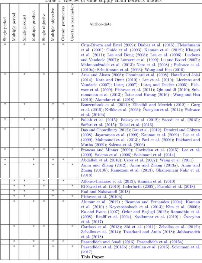
League Champion meta-heuristic algorithm in their solution approach. Alamdar et al. (2018) investigate the optimal decisions in CLSC under a fuzzy price and sales effort-dependent demand. They establish several game theory models to compare the behavior of a manufacturer, a retailer and a collector. Farrokh et al. (2018) use a fuzzy stochastic programming approach to a supply chain design while Jabbarzadeh et al. (2018) use a robust approach to design CLSC under operational and disruption risks. Soleimani et al. (2017) consider a green CLSC design accounting for environmental considerations, as well as lost working days and propose a genetic algorithm for solution method, and Rad and Nahavandi (2018) consider also a green multi objective CLSC whose objective functions are the economic cost, and environmental emissions,and of customer satisfaction. They develop an ant colony optimization solution algorithm for their model. Tosarkani and Amin (2018) conduct a Fuzzy analytic network process in a case study of battery supply chain design, while in another case study, ¨Ozceylan et al. (2017) develop a linear programming model for CLSC of the automotive industry in Turkey. A more detailed classification based on four factors including the certain and uncertain parameters, single and multi-period models, single and multi-product models, and single and multi-objective models is illustrated in Table 1.
Contribution highlights
The above literature review reveals that to the best of our knowledge there is no model in the supply chain network designs that takes into account all uncertain parameters involved in many real-world environments. In order to make the model more applicable, the present study develop a comprehensive model to consider customer demand in each period, transportation costs of raw materials and products, purchase price of the raw materials, shortage costs, and fraction of the returned products as uncertain parameters. Unlike other studies, the selected facilities in each period are capable of getting opened and closed by applying some relevant costs. In addition, the proposed model seeks to minimize the total costs among uncertain parameters. It must be mentioned that the designed model is developed based on RFP. To approach the model, a novel WOA algorithm is proposed using a modified priority-based encoding to find an approximate optimal solution within a reasonable computational time.
Table 1: Review of some supply chain network models Single p erio d Multiple p erio d Single pro duct Multiple pro duct Single ob jectiv e Multiple ob jectiv e Certain parameters Unertain parameters Author-date
* * * * Cruz-Rivera and Ertel (2009); Diabat et al.(2015);Fleischmann et al. (2001); Guide et al.(2003); Kannan et al.(2012);Khajavi et al. (2011); Lee and Dong (2008); Lee et al. (2006); Lieckens and Vandaele(2007);Louwers et al.(1999);Lu and Bostel(2007); Mahmoudzadeh et al.(2013);Neto et al.(2008) ; Pishvaee et al. (2010a);Schultmann et al.(2003);Wang and Hsu(2010)
* * * * Aras and Aksen(2008);Chouinard et al.(2008);Hatefi and Jolai (2014); Kara and Onut (2010) ; Lee et al. (2010); Lieckens and Vandaele (2007); Liste¸s(2007); Liste¸s and Dekker (2005); Pish-vaee et al.(2009);Pishvaee et al.(2011);Qin and Ji(2010); Sub-ramanian et al.(2013);Uster and Hwang¨ (2016) ;Wang and Hsu (2010);Alamdar et al.(2018)
* * * * Bouzembrak et al. (2011); Elhedhli and Merrick (2012) ; Garg et al.(2015);Krikke et al.(2003);Ozceylan et al.¨ (2014);Pishvaee et al.(2010b)
* * * * Fallah et al. (2015); Paksoy et al. (2012); Saeedi et al. (2015); Saffari et al.(2015);Talaei et al.(2016)
* * * * Das and Chowdhury(2012);Dat et al.(2012);Demirel and G¨ok¸cen (2008);Jayaraman et al.(1999);Kannan et al.(2009) ;Lee et al. (2009);Mahmoudi et al.(2013); Pati et al.(2006);Pokharel and Mutha(2009);Salema et al.(2006)
* * * * Francas and Minner (2009); Govindan et al. (2015); Lee et al. (2009);Salema et al.(2006);Soleimani et al.(2014)
* * * * Abdallah et al.(2010);Uster et al.¨ (2007);Wang et al.(2011) * * * * Amin and Zhang (2012); Amin and Zhang (2013a); Amin and
Zhang(2013b); Ramezani et al. (2013); Ghahremani Nahr et al. (2018)
* * * * Alfonso-Lizarazo et al.(2013);Kannan et al.(2010)
* * * * El-Sayed et al.(2010);Inderfurth(2005);Farrokh et al.(2018) * * * * Rad and Nahavandi(2018)
* * * * Pishvaee et al.(2010b)
* * * * Alumur et al. (2012) ; Beamon and Fernandes (2004); Kannan et al. (2010) ; Keyvanshokooh et al. (2013); Kim et al. (2006); Ko and Evans(2007);Ozkır and Ba¸slıgıl¨ (2012);Ramudhin et al. (2008); Realff et al.(2004); Sasikumar et al. (2010) ; Ozceylan¨ et al.(2017)
* * * * Cardoso et al. (2013); Shi et al. (2011); Zeballos et al. (2012); Zeballos et al. (2014); Tosarkani and Amin (2018); Jabbarzadeh et al.(2018)
* * * * Pasandideh and Asadi(2016);Pasandideh et al.(2015a)
* * * * Pasandideh et al.(2015b) ;Subulan et al.(2015);Soleimani et al. (2017)
This Paper
3
Problem definition and mathematical formulation
In this problem, a multi-product, multi-period, multi-echelon CLSC network is designed under discounts, shortage, and uncertainty. Our research was first motivated from a local automotive manufacturer in Iran. However, we state it as a general problem without speaking of a specific product since the model is capable of addressing different
manufac-turing sectors with similar frameworks with slight customization as already have also been discussed in the literature for several other industries. Among those are, electronics and digital equipment (Rad and Nahavandi 2018; Amin and Baki 2017); battery (Tosarkani and Amin 2018); tire (Amin et al. 2017; Sahebjamnia et al. 2018); e-commerce in an Indian firm (Prakash et al. 2018); yarn, fabric, and apparel (Kim et al. 2018); glass (Hajiaghaei-Keshteli and Fard 2018); washing machine (Jeihoonian et al. 2017).
The description of our supply chain network is given as follows. The forward flow net-work includes raw-material suppliers, production centers, warehouses, distribution cen-ters, and customer zones. The reverse network includes collection cencen-ters, repair cencen-ters, recycling and disposal centers, as well as all facilities with limited capacities. As it is il-lustrated in Figure1, in the forward flow network, the raw-material suppliers ship the raw materials needed to produce the new products in the production centers. The raw ma-terials are sent to the warehouses after being processed in the production centers. Then, distribution centers deliver them to final customers. In the reverse flow, a proportion of the products returned from the customers is collected by the collection centers, where fixable products are sent to repair centers after inspection. The rest is sent to a recycling center. The repaired products at the repair centers, as new ones, are sent back to the distribution centers and the potential warehouses. In addition, recyclable products after disassembly at recycling centers are sent to the production center for reuse (if they could be reused); otherwise, they are sent to disposal centers.
S S S S M W E M W E L U R C C C C C Figure 1: A multi-echelon CLSC network
To specify the study scope, the following assumptions are made to formulate the problem:
• The discount offered by the raw material supplier is of a quantity discount type.
• The location of all centers has to be determined.
• Unmet demand of customers (shortage) is back-ordered.
• Customer demand of each product must be satisfied until the last time period.
• Distribution and collection centers are considered as hybrid centers.
• The customer demand, fraction of returned product, transportation cost between facilities, purchase cost, and shortage cost are considered as uncertainty parameters. With consideration of the above-mentioned assumptions, the most important issues addressed in this paper are as follow:
• To locate the raw material supplier, production centers, warehouses, hybrid distri-bution/ collection centers, repair centers, recycling centers, and disposal centers
• To determine the optimal flow between the located centers
• To find an appropriate level of discount.
The following subsections define the notations used the formulation of our proposed model.
3.1 Sets
Symbol Definition index
S Set of raw-material suppliers ∀s∈S
M Set of production centers ∀m∈M
W Set of potential warehouses ∀w∈W E Set of distribution/collection centers ∀e∈E
C Set of customer zone ∀c∈C
R Set of repair centers ∀r∈R
U Set of recycling centers ∀u∈U
L Set of disposal centers ∀l∈L
T Set of periods ∀t∈T
P Set of products ∀p∈P
I Set of raw-materials ∀i∈I
H Set of discount levels ∀h∈H
The following sets are also defined to offer definitions of the model parameters and the decision variables: G1 =S∪M∪W ∪E∪C A0 ={(i, j)|(i∈M, j ∈W)∪(i∈W, j ∈E)∪(i∈E, j ∈C)} A00 ={(i, j)|(i∈S, j ∈M)} G2 =C∪E∪R∪U ∪L A000 ={(i, j)|(i∈C, j ∈E)∪(i∈E, j ∈R)∪(i∈E, j ∈U)∪(i∈R, j∈E)∪(i∈R, j ∈ W)} A0000 ={(i, j)|(i∈U, j ∈L)∪(i∈U, j ∈M)} G= (G1 ∪G2)\C A1 =A00∪A0000 and A2 =A0∪A000. 3.2 Parameters
fjt The fixed cost of facilityj ∈Gin period t opjt The opening cost of facility j ∈G in period t cljt The closing cost of facility j ∈Gin period t tc1
ijj0n Unit transportation cost of raw-material i between facilities (j, j0) ∈ A1 with
transportation mode n
tc2pjj0n Unit transportation cost of product p between facilities (j, j0)∈A2 with
trans-portation moden
himt Unit inventory holding cost of raw-materialiby production centerm in period t
h0pwt Unit inventory holding cost of productm by potential warehouse w in period t
prisht Unit purchase cost of raw-material iby raw-material supplier s with discount level h in period t
vaisht Lower limit on the business volume of raw materiali by raw-material supplier s that corresponds to the discount interval h in period t (vai,s,1,t = 0,∀s, i, t) c1
pmt Unit production of productp by production center m in period t c2
pet Unit distribution cost of productpby distribution/collection centerein period t
c3
pet Unit collection cost of returned product p by distribution/collection center e in period t
c4
prt Unit repair cost of product p by repair center r in period t c5
put Unit recycling cost of product p by recycling center u in period t c6ilt Unit disposal cost of raw-material iby disposal center l in period t
πpct Unit shortage cost of product p in supplying demand of customer zone c in period t
δip The number raw-material i needed to produce a unit of product p dempct Demand of product p of customer zone cin period t
αpct Fraction of returned product pfrom customer zone cin period t βpt Fraction of repairable product p in period t
γpt Fraction of repaired productpin periodtthat sends to distribution/collection center
θit Fraction of usable raw-material i in period t cap1
si Capacity of supplier s for raw-materiali cap2
mi Capacity of production center m of raw-material i cap3
mp Capacity of production center m of product p cap4wp Capacity of potential warehouse w of product p cap5ep Capacity of distribution center e of product p cap6
wp Capacity of distribution center e of product p cap7
rp Capacity of repair center r of product p cap8
up Capacity of recycling center u of product p cap9
li Capacity of disposal center l of raw-material i
3.3 Decision variables
X1
ijj0nt Quantity of raw-material i shipped between facilities (j, j0) ∈ A1 with
transportation mode n in period t X2
ijj0nt Quantity of product p shipped between facilities (j, j0)∈ A2 with
trans-portation mode n in period t
Qist Total quantities ordered for raw material i from supplier s in period t over the planning horizon
IQpwt Quantity of productp stored at potential warehouse w in period t U Dpct Quantity of non-satisfied demand of product p of customer cin period t Yjt 1 if facility j ∈Gis opened in periodt; 0 otherwise.
Aisht 1 if the quantity purchased of raw material i from supplier s in period t falls in the discount intervalh; 0 otherwise
3.4 Deterministic modeling
The deterministic mathematical model of the problem can be presented as follows.
minZ =X t∈T X j∈G (fjtYjt+opjtYjt(1−Yj,t−1) +cljtYjt(1−Yj,t+1)) + X n∈N X i∈I X (j,j0)∈A 1 tc1ijj0nXijj1 0nt+ X p∈P X (j,j0)∈A 2 tc2pjj0nXpjj2 0nt +X i∈I X j∈M hijtV Qijt+ X p∈P X j∈W h0ijtIQpjt+ X p∈P X j∈C πpjtU Dpjt +X i∈I X j∈S X j0∈M X h∈H X n∈N
prijhtAijhtXijj1 0nt
+X p∈P X n∈N X j∈M X j0∈W c1pjt+X j∈E X j0∈C c2pjt+X j∈C X j0∈E c3pj0t+ X j∈E X j0∈R c4pj0t + X j∈E X j0∈U c5pj0t Xpjj2 0nt+ X i∈I X j∈U X j0∈L X n∈N c6j0itXijj1 0nt (1) s.t.
Aijhtvaijht ≤Qijt, ∀j ∈S, h∈H, i∈I, t ∈T (2)
X h∈H Aijht =Yjt, ∀j ∈S, i∈I, t∈T (3) Qijt= n∈N X j0∈M Xijj1 0nt, ∀j ∈S, i∈I, t ∈T (4) X j∈S X n∈N Xijj1 0nt+ X j∈U X n∈N Xijj1 0nt+V Qij0,t−1− X p∈P X j∈W X n∈N Xpj20jntδip =V Qij0t, ∀j0 ∈M, i∈I, t∈T (5) X j∈M X n∈N Xpjj2 0nt+ X j∈R X n∈N Xpjj2 0nt+IQpj0,t−1− X j∈E X n∈N Xpj20jnt =IQpj0t, ∀j0 ∈W, p∈P, t∈T (6) X j∈W X n∈N Xpjjnt2 +X j∈R X n∈N Xpjj2 0nt = X j∈C X n∈N Xpj20jnt, ∀j0 ∈E, p∈P, t∈T (7)
X j∈E X n∈N Xpjjnt2 −U Dpj0,t−1+U Dpj0t =dempj0t, ∀j0 ∈C, p∈P, t∈T (8) αpj0t X j∈E X n∈N Xpjj2 0n,t−1 = X j∈E X n∈N Xpj20jnt, ∀j0 ∈C, p∈P, t∈T (9) βpt X j∈C X n∈N Xpjj2 0nt = X j∈U X n∈N Xpj20jnt, ∀j0 ∈E, p∈P, t∈T (10) (1−βpt) X j∈C X n∈N Xpjj2 0nt = X j∈U X n∈N Xpj20jnt, ∀j0 ∈E, p∈P, t∈T (11) γpt X j∈E X n∈N Xpjj2 0nt = X j∈E X n∈N Xpj20jnt, ∀j0 ∈R, p∈P, t∈T (12) (1−γpt) X j∈E X n∈N Xpjj2 0nt = X j∈W X n∈N Xpj20jnt, ∀j0 ∈R, p∈P, t∈T (13) θit X p∈P X j∈E X n∈N Xpjj2 0ntδip= X i∈I X j∈M X n∈N X11j0jnt, ∀j0 ∈U, i∈I, t ∈T (14) (1−θit) X p∈P X j∈E X n∈N Xpjj2 0ntδip = X p∈P X j∈L X n∈N XIj10jnt, ∀j0 ∈U, i∈I, t∈T (15) X j0∈M X n∈N Xijj1 0nt ≤cap1jiYjt, ∀j ∈S, i∈I, t∈T (16) V Qijt ≤cap2jiYjt, ∀j ∈M, p∈P, t∈T (17) X j0∈W X n∈N Xpjj2 0nt ≤cap3jpYjt, ∀j ∈W, p∈P, t∈T (18) IQpjt ≤cap4jpYjt, ∀j ∈W, p∈P, t∈T (19) X j∈W X n∈N Xpjj2 0nt+ X j∈R X n∈N Xpjj2 0nt ≤cap5j0pYj0t, ∀j0 ∈E, p∈P, t∈T (20) X j∈C X n∈N Xpjj2 0nt ≤cap6j0pYj0t, ∀j0 ∈E, p∈P, t∈T (21) X j∈E X n∈N Xpjj2 0nt ≤cap7j0pYj0t, ∀j0 ∈U, p∈P, t∈T (22) X j∈E X n∈N Xpjj2 0nt ≤cap8j0pYj0t, ∀j0 ∈R, p∈P, t∈T (23) X j∈U X n∈N Xijj1 0nt ≤cap9j0iYj0t, ∀j0 ∈L, p∈P, t∈T (24) V Qim,0 = 0, ∀i∈M, t= 1 (25) IQpw,0 = 0, ∀j ∈W, t=T (26) U Dpc,0 = 0, ∀j ∈P, t=T (27)
Xijj1 0nt, V Qimt, Qist ≥0, ∀(j, j0)∈A1, i∈I, n∈N, t∈T, s∈S, m∈M (28)
Xpjj2 0nt, IQpmt, U DP Ct ≥0, ∀(j, j0)∈A2, p∈P, n∈N, t∈T, w∈W, c∈C (29)
The objective function (1) intends to minimize the total supply chain network costs including the annual fixed costs, costs of opening and closing the facilities (first row), transportation costs of raw materials and manufactured products (second row), holding costs of raw materials and finished products, as well as the shortage penalty cost (third row), raw material cost associated with the discount (fourth row) operational costs asso-ciated with the facilities as the cost of producing, distributing, collecting, repairing and recycling, respectively (in the fifth row), and finally disposal of products. The constraint in inequality (2) represents the total amount of raw materials purchased from the suppli-ers at their expressed discount levels. Constraint (3) ensures that the selected supplier purchases the raw materials at only one discount interval. Constraint (4) sends the total raw materials purchased from the suppliers to the production centers. Constraint (5) presents the volume of raw materials sent by the supplier and recycling centers to the plant, where a portion is stored in the warehouse of the factory after production. Con-straint (6) controls the input and output volumes of the warehouse. Equation (7) is a balance constraint on the distribution center and ensures that the input flow from the repair center and warehouse to the repair center is equal to the output flow from the distribution center to the customers. Constraint (8) guarantees that customer demand must be met till the last moment. Constraint (9) presents a percentage of products which are returned a period after being bought by customers. Constraints (10)–(11) indicate that the proportion of repairable goods which are sent from collection centers to the re-pair center and the proportion of irreparable ones to the recycling centers after inspection in the collection centers. Constraints (12) indicates that a portion of repaired items are returned back to the distribution centers while (13) shows that the rest of the repaired items is sent to warehouses. Similarly, constraints (14) shows the portion of recycled raw material which are re-sent to the manufacturing centers after inspection and disassembling the products while (15) shows the rest of them that are sent to the the disposal centers. Constraints (16)-(17) are related to the capacity of the network facilities, i.e. the capacity of the supplier in raw material procurement, the amount of storage of each raw material in the warehouse, and the production capacity of each product for created factories, re-spectively. Constraint (19) ensures that if a warehouse is established, its capacity cannot exceed the predetermined capacity. Constraints (20)–(21) state that if dual collection and recycling centers are created, the amount of distribution and collection does not exceed
the capacity of the facility while constraint (22) shows the maximum ability for recycling the products at the recycling center. Constraint (23) indicates the maximum capacity of the repair centers in terms if number of products and similarly, Constraint (24) restricts disposal amount of unusable raw materials. Constraints (25)–(27) set the initial value of raw material, finished product and back orders. Finally, constraints (28)–(30) define the type of decision variables and their range.
3.5 Uncertainty modeling
3.5.1 Trapezoidal fuzzy programming model
To tackle uncertainty parameters in the objective function and constraints, some fuzzy models such as chance constraint fuzzy programming (FP) have been developed. It is a well-recognized method that relies on profound mathematical concepts such as the expected value of a fuzzy number in the objective function and possibility and the necessity measure in the constraints. Inuiguchi and Ramık (2000) propose various fuzzy number forms such as triangular and trapezoidal fuzzy number to support uncertain model. Here we use the trapezoidal fuzzy distribution to show the basic FP model and the necessity measure to control the conservatism level of satisfying the constraints. Consider the following mathematical model as the base:
(FP1) minZ =ax+f y (31a)
s.t.
bix≥ci, ∀i= 1, ..., l (31b)
dix=eiy, ∀i= 1, ..., m (31c)
x, y ≥0. (31d)
Suppose vectora(variable costs),c(customer demand), and coefficient matrixd (frac-tion of the returned product) are the uncertain parameters of the problem. So, to con-struct its FP counterpart model and tackle the uncertainty parameters, the expected value and necessity measure are made use of in the objective function and constraints, respectively. The necessity measure is used to convert fuzzy chance constraints into their equivalent crisp ones. Eq. (32) expresses the membership function of a trapezoidal fuzzy
number, ˜a, by four sensitive points (i.e. ˜a(p),a˜(rp),˜a(ro),a˜(o)) shown on Figure 2. µ˜a(x) 0, x < p x−ap arp−ap, p≤x≤rp a0−x a0−aro, ro≤x≤o 0, x≥o. (32) ˜ a 1 ˜ a(p) ˜a(rp) a˜(ro) ˜a(o)
Figure 2: Fuzzy parameter ˜a
Therefore, the following model which all fuzzy parameters defined as trapezoidal ones is considered as the FP counterpart expression for (31a–31d):
(FP2) minZ = ˜atx+f y (33a)
s.t.
N EC(bix≥ci)≥ϑn, ∀i= 1, ..., l (33b) N EC( ˜dix=eiy)≥ϑn, ∀i= 1, ..., m (33c)
x, y ≥0. (33d)
Knowing that uncertainty parameters of the constraints must be formed with a satisfaction level of at least ϑn, the equivalent crisp parametric model of (33a–33d) can be written as follows: (CFP) minEV[Z] = ap+arp +aro+ao 4 x (34a) s.t. bix≥(1−ϑn)ciro+ (ϑn)coi, ∀i= 1, ..., l (34a) [(ϑn)d rp i + (1−ϑn)d p i]x≤eiy, ∀i= 1, ..., m (34b)
[(ϑn)doi + (1−ϑn)droi ]x≥eiy, ∀i= 1, ..., m (34c)
x, y ≥0, 0≤ϑn ≤1. (34d)
According to the above-presented descriptions, the equivalent auxiliary crisp model of the CLSC network design model, given in (1–30), can be formulated as follows:
minEV[Z] =X t∈T X j∈G (fjtYjt+opjtYjt(1−Yj,t−1) +cljtYjt(1−Yj,t+1)) + X (j,j0)∈A 1 X i∈I X n∈N 1 4
tc1ijjp0n+tc1ijjrp0n+tc1ijjro0n+tc1ijjo0n
Xijj1 0nt + X (j,j0)∈A 2 X p∈P X n∈N 1 4
tc2ijjp0n+tc2ijjrp0n+tc2ijjro0n+tc2ijjo0n
Xpjj2 0nt + X j∈W X p∈P h0ijtIQpjt+ X j∈M X i∈I X t∈T hijtV Qjit +X j∈C X p∈P 1 4 πpjtp +πpjtrp +πpjtro +πpjto U Dpct +X j∈S X j0∈M X i∈I X n∈N X h∈H 1 4
prpijht+prrpijht+prroijht+proijhtAijhtXijj1 0tn
+X p∈P X n∈N X j∈M X j0∈W c1pjt+X j∈E X j0∈C c2pjt+X j∈E X j0∈C c3pjt+X j∈E X j0∈R c4pjt + X j∈E X j0∈U c5pjt Xpjj0nt+ X j∈U X j0∈L X i∈I X n∈N c6ij0tXijj0nt s.t. X j∈E X n∈N Xpjj0nt−U Dpj0,t−1+U Dpj0t≥(1−ϑ1)demro pj0t+ (ϑ1)demopj0t, ∀j0 ∈C, p∈P, t∈T (35) h (ϑ2)αrppj0t+ (1−ϑ2)αppj0t i X j∈E X n∈N Xpjj2 0n,t−1 ≤ X j∈E X n∈N Xpj20jnt, ∀j0 ∈C, p∈P, t∈T (36) h (ϑ2)αopj0t+ (1−ϑ2)αropj0t i X j∈E X n∈N Xpjj2 0n,t−1 ≤ X j∈E X n∈N Xpj20jnt, ∀j0 ∈C, p∈P, t∈T (37) 0.5≤ϑ1, ϑ2 <1 (38) (10)–(30).
3.5.2 The proposed robust fuzzy programming
Now, we present the robust formulation of the obtained fuzzy mathematical model. As-suming again that only vectors a, c, and the coefficient matrix d are the uncertain pa-rameters, according to the (CFP) model, the (RFP) model is formulated as follows:
(RFP) minE[Z] =EV[Z] +ω(Zmax−Zmin) +ρ[coi −(1−ϑn)croi −(ϑ)c o i] +τ[droi + (ϑn)drpi + (1−ϑn)dip−(ϑn)doi −(1−ϑn)droi −d p i] (39a) s.t. bix≥(1−ϑn)ciro+ (ϑn)coi, ∀i= 1, ..., l (39b) [(ϑn)drpi + (1−ϑn)dpi]x≤eiy, ∀i= 1, ..., l (39c) [(ϑn)doi + (1−ϑn)droi ]x≥eiy, ∀i= 1, ..., m (39d) x, y ≥0, 0≤ϑn ≤1. (39e)
Similar to (CFP) model, the first term in the objective function is the expected value of Z, which results in minimization of the expected total network costs. The second term, i.e., ω(Zmax−Zmin), indicates the difference between the two extreme possible values of Z where ω represents the weight of this term against the three other terms in objective function. Moreover, Zmax and Zmin can be defined as follows:
Zmax =aox+f y (40a)
Zmin =apx+f y (40b)
Therefore, the existence of the second term results in controlling the optimality robustness of the solution vector under the expected optimal value of Z. The third and fourth terms determine the confidence level of each chance constraint. ρ and τ are the unit penalty of possible violation of each constraint, and [coi −(1−ϑn)croi −(ϑn)coi] and [droi + (ϑn)drpi + (1−ϑn)dpi −(ϑn)doi−(1−ϑn)droi −d
p
i] indicate the difference between the worst case value of uncertainties parameters in chance constraints. Therefore, the proposed robust fuzzy programming model for CLSC network design is as follows:
+X c∈C X p∈P X t∈T nh
democpt −(1−ϑ1)demrocpt−(ϑ1)democpt
i +τhαropct+ (ϑ1)αrppct+ (1−ϑ1)αpctp −(ϑn)αpcto + (1−ϑ1)αropct−α p pct io (41) s.t. Zmax = X t∈T X j∈G (fjtYjt+opjtYjt(1−Yj,t−1) +cljtYjt(1−Yj,t+1)) (42) + X n∈N X i∈I X (j,j0)∈A 1 tc1ijjo0nXijj1 0nt+ X p∈P X (j,j0)∈A 2 tc2pjjo 0nXpjj2 0nt +X i∈I X j∈M hijtV Qijt+ X p∈P X j∈W h0ijtIQpjt+ X p∈P X j∈C πpjto U Dpjt +X i∈I X j∈S X j0∈M X h∈H X n∈N
proijhtAijhtXijj1 0nt
+X p∈P X n∈N X j∈M X j0∈W c1pjt+X j∈E X j0∈C c2pjt+X j∈C X j0∈E c3pj0t+ X j∈E X j0∈R c4pj0t + X j∈E X j0∈U c5pj0t Xpjj2 0nt+ X i∈I X j∈U X j0∈L X n∈N c6j0itXijj1 0nt (43) Zmin = X t∈T X j∈G (fjtYjt+opjtYjt(1−Yj,t−1) +cljtYjt(1−Yj,t+1)) (44) + X n∈N X i∈I X (j,j0)∈A 1 tc1ijjp0nXijj1 0nt+ X p∈P X (j,j0)∈A 2 tc2pjjp 0nXpjj2 0nt +X i∈I X j∈M hijtV Qijt+ X p∈P X j∈W h0ijtIQpjt+ X p∈P X j∈C πpjtp U Dpjt +X i∈I X j∈S X j0∈M X h∈H X n∈N
prpijhtAijhtXijj1 0nt
+X p∈P X n∈N X j∈M X j0∈W c1pjt+X j∈E X j0∈C c2pjt+X j∈C X j0∈E c3pj0t+ X j∈E X j0∈R c4pj0t + X j∈E X j0∈U c5pj0t X 2 pjj0nt+ X i∈I X j∈U X j0∈L X n∈N c6j0itXijj1 0nt (45) (10)–(30),(35)–(38).
The proposed RFP model is a MINLP model. The NP-hardness of supply chain network design problem has been proved in a good number of studies (e.g., Jayaraman et al. 2003). They consist of two different parts, i.e. facility location problem and quantity flow optimization among facilities and therefore, they are reducible to facility location problems which have been proved to be NP-complete by Davis and Ray (1969). So the discussed CLSC network design problem is considered as NP-hard in the present
study. Approaching this problem in large sizes by exact solutions is very time-consuming and sometimes impractical. Therefore, several meta-heuristic algorithms with different representations have been developed to obtain near-optimal solutions; though all the proposed algorithms are not efficient. In the present study, a WOA algorithm based on modified priority-based encoding was applied, which will be described in the following section.
4
Solution approach
While exact methods used to be a good way for solving problems, ranging from linear problems to non-linear problems, the recent decades have seen an increase in the number of heuristic and meta-heuristic approaches to solve very complex problems. Using exact approaches to solve problems which have a large scale seems not to be the best way therefore, researchers have inclined to use heuristic and meta-heuristic approaches to solve complex problems. In other words, the exact solution methods are ineffective to find the optimum solution for large scale problems so, it has set the stage for solving problems by heuristic and meta-heuristic approaches. Here we present a new population-based meta-heuristic optimization algorithm inspired from animal behavior, called WOA using modified a new priority-based encoding in order to cover the feasible search space. On the other hand we present the corresponding decoding approach for solving the designed CLSC network.
4.1 Solution representation (priority based encoding)
The debate about solution presentation is both timely and crucial. The path towards encoding and decoding may be steep and strewn with challenges, which affect the algo-rithms to find the optimum solution in the feasible solution space. Tree-based solution is one way of representing supply chain network design problems. Gen and Cheng (2000) introduced three ways of encoding tree, contains edge-based encoding, vertex-based en-coding, and edge-vertex enen-coding, however, there are several other ways of encoding tree. In this paper, we have used vertex-based encoding which is modified in order to solve the CLSC network problem. Furthermore, a priority-based encoding developed is based on the work of Gen and Cheng (2000). The most noticeable about this encoding is that it can solve the quantity flow optimization, facility location problem and proper amount
shortage in each period simultaneously. We consider two-level supply chain network as shown in Figure 3 with (|K|) sources and (|J|) depots. The length of this solution is equal to|K|+|J|and the location of each cell represents the priorities in each period. We regard two different procedures for decoding the solution, ranging from forward to reverse supply chain. The variation between these two procedures are related to the potential sources that must be located. The shortage of demand in the forward supply chain, may lead to less number of source location than that of the time at which all demand must be satisfied. On the other hand, all the returned products, must be collected in forward supply chain, which means that the number of sources should be such that capacity of located sources be able collect all returned products. In the following we explained the decoding procedures of solutions for forward and reverse supply chain.
Transportation cost 4 3 1 6 2 5 3 1 3 7 5 2 Source 1 220 2 210 3 240 Depot 1 120 2 150 3 130 4 180
Figure 3: Sample of two-level supply chain network
4.1.1 The decoding of the solutions for forward supply chain
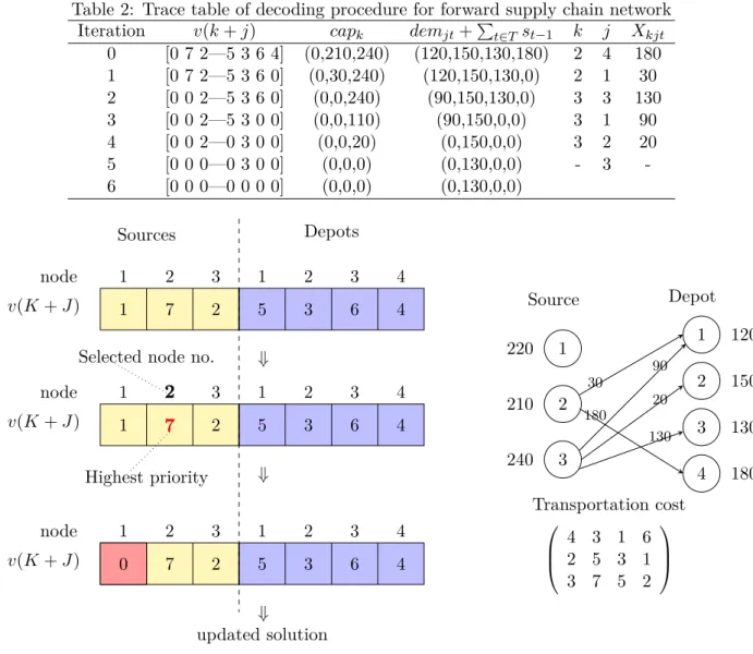
In the first stage of the process, we select the cell number with the highest priority among sources as a number of sources that must be opened. Then, we select the highest prior-ities among sources and reduce the other priorprior-ities to zero. The next stage is updating the solution, in which before connecting to a node (source or depot) with the minimum transportation cost, select the node (depot or source) with the highest priority. Subse-quently, determining the amount of shipment between the selected nodes by calculating minimum of the total demand and the shortage of previous periods, and capacity. Next, the priority of depot or source is reduced to zero. If total demand of depots is greater than total capacity of the selected sources, the amount of shortage for each depot is calcu-lated. This process is repeated until all priorities are equal to zero. Table 2 presents the trace table for the forward supply chain network, and Figure 4 shows how this modified priority-based encoding is obtained.
Table 2: Trace table of decoding procedure for forward supply chain network Iteration v(k+j) capk demjt+Pt∈T st−1 k j Xkjt
0 [0 7 2—5 3 6 4] (0,210,240) (120,150,130,180) 2 4 180 1 [0 7 2—5 3 6 0] (0,30,240) (120,150,130,0) 2 1 30 2 [0 0 2—5 3 6 0] (0,0,240) (90,150,130,0) 3 3 130 3 [0 0 2—5 3 0 0] (0,0,110) (90,150,0,0) 3 1 90 4 [0 0 2—0 3 0 0] (0,0,20) (0,150,0,0) 3 2 20 5 [0 0 0—0 3 0 0] (0,0,0) (0,130,0,0) - 3 -6 [0 0 0—0 0 0 0] (0,0,0) (0,130,0,0) Source 1 220 2 210 3 240 Depot 1 120 2 150 3 130 4 180 30 180 90 20 130 Transportation cost 4 3 1 6 2 5 3 1 3 7 5 2 Sources Depots 1 2 3 1 2 3 4 1 7 2 5 3 6 4 ⇒ node v(K+J) 1 2 3 1 2 3 4 1 7 2 5 3 6 4 ⇒ node v(K+J) 1 2 3 1 2 3 4 1 7 2 5 3 6 4 ⇒ node v(K+J) 0 7 Highest priority 2
Selected node no.
updated solution
Figure 4: Sample of two-level supply chain network
This decoding process is conducted in the specific framework; its decoding algorithm as well as calculation table in the first period is illustrated in Algorithm 1.
4.1.2 The decoding of the solutions for reverse supply chain
Once again, consider the two-level supply chain network that shown in Figure3. To decode the solution, in the first section, the cell with the highest priority among source nodes is selected, then if capacity of the selected source is less than total returned products the next highest priority is also selected. This procedure will continue while the total capacity of sources is less than total returned products of depots. In the next stage, the priorities of the nodes which are not selected are decrease to zero. Then, select the node (depot or source) with the highest priority and connect it with the node which has the minimum transportation cost. After that, the amount of shipment between the selected
Algorithm 1 Decoding algorithm of forward supply chain network
Require: Sets of K, J, T; The demand, capacity and transportation costs; encoded solution
v(K+J)
Ensure: Xkjt: Quantity of shipment between source kand depotj Sjt: Shortage of depot j in periodt Ykt: Opening of a center at locationk in periodt
1:
2: fort= 1 to T do
3: Select a node onl= arg max{v(k),∀k∈K}, so that P
k∈KYkt=l 4: while|d|< l do
5: Select a node ond= arg max{v(k), k∈K} 6: if |d|=l then v(k−l) = 0,∀k∈K, l∈L 7: tr(k−l),i=∞,∀j∈ |J|, k∈K, l∈L 8: cap(k−l)=0, ∀k∈K,l∈L 9: end while 10: whilev(|k|+j)6= 0,∀j∈J do 11: Xkjt= 0, Sjt = 0,∀j∈J, k∈K, t∈T
12: Select a node based on l= arg max{v(t), t∈ |K|+|J|},∀j ∈J, k∈K
13: if l∈K a source is selectedk∗ =l then
14: j∗ = arg min{trkj|v(j)6= 0}∀j∈J select a depot with minimum cost 15: else if l∈j a depot selected j∗ =l then
16: k∗= arg min{trkj|v(j)6= 0}∀k∈K select a source with minimum cost 17: end if
18: Update demands and capacities:
19: Xk∗j∗t= min(capk∗, demj∗t+Sj∗t)
20: capk∗ =capk∗−Xk∗j∗t
21: demj∗t=demj∗t+S(j∗t−1)−X(k∗j∗t)Step 8.
22: if capk∗ = 0 then v(k∗) = 0
23: if demj∗t= 0 then v(j∗) = 0
24: end while 25: if P
jXkjt>0 then Ykt= 1
26: if demjt>0 then Sjt =Sj,t−1+demjt 27: end for
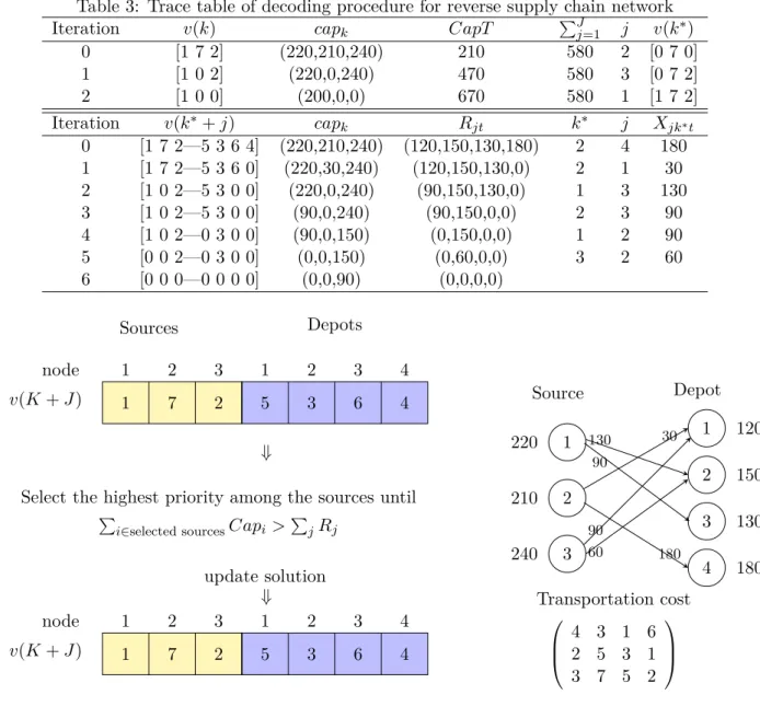
nodes is determined by taking the minimum of returned products and capacity. Then the priority (depot or source) is reduced to zero and this process is repeated until all priorities equal to zero. Table 3 presents the trace table for the reverse supply chain network, and Figure5demonstrates how its modified priority-based encoding is obtained. The decoding algorithm of solution for a reverse supply chain network is also given in Algorithm 2.
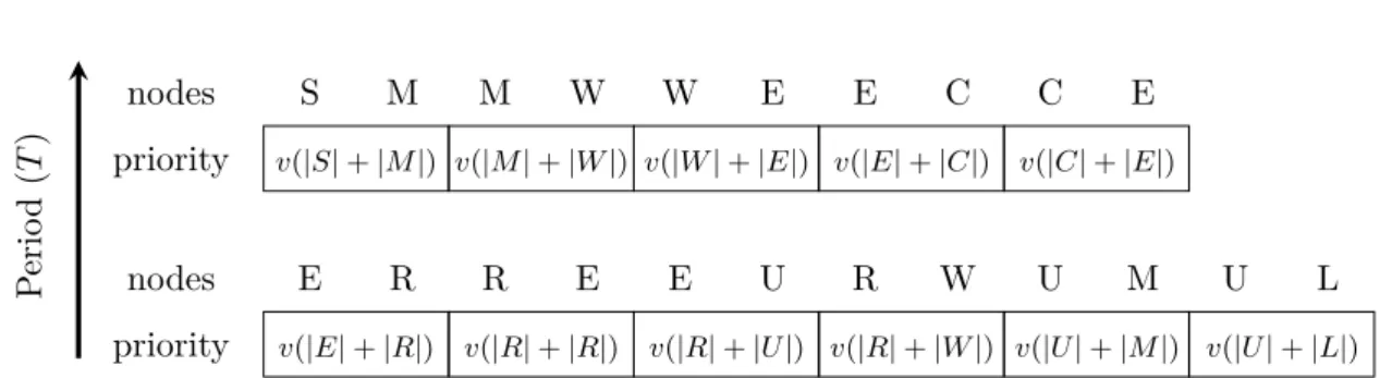
In this paper, as mentioned before, the problem is a level, product, multi-period CLSC network design, and the proposed solution should consider these items. Therefore, as illustrated in Figure 6, the priority based encoding is represented by a matrix, where T is a number of time periods, P is a number of products,S is a number of raw material supplier, M is a number of production centers, W is a number of potential warehouses, E is a number of hybrid distribution/collection centers, R, U, L are the numbers of repair centers, recycling centers, and disposal centers, respectively.
Algorithm 2 Decoding algorithm of reverse supply chain network
Require: Sets of K, J, T; The returned product, capacity and transportation costs; encoded solution v(K+J)
Ensure: Xkjt: Quantity of shipment between source kand depotj Ykt: Opening of a center at locationk
1: Step1.
2: fort= 1 to T do 3: whilecapT =PJ
j=1Rjt do
4: Select a node onl= arg max{v(k), k∈K} 5: capT =PK l=1capl 6: if capT <PJ j=1Rjt then 7: v(k−l) = 0,∀k∈K, l∈L 8: trj,(k−l) =∞ ∀j∈J, k∈K, l∈L 9: end if 10: end while 11: whilev(|k|+j)6= 0,∀j∈J do 12: Xkjt= 0, Sjt = 0,∀j∈J, k∈K
13: Select a node based on l= arg max{v(t), t∈ |K|+|J|},∀j ∈J, k∈K
14: if l∈K a source is selectedk∗ =l then
15: j∗ = arg min{trkj|v(j)6= 0}∀j∈J select a depot with minimum cost 16: else if l∈j a depot selected j∗ =l then
17: k∗= arg min{trkj|v(j)6= 0}∀k∈K select a source with minimum cost 18: end if
19: Update demands and capacities: 20: Xk∗j∗t= min(capk∗, Rj∗t) 21: capk∗ =capk∗−Xk∗j∗t 22: Rj∗t=Rj∗t−X(k∗j∗t) 23: if capk∗ = 0 then v(k∗) = 0 24: if Rj∗t= 0 then v(j∗) = 0 25: if P jXkjt >0 then Ykt= 1 26: end while 27: end for
4.2 The whale optimization algorithm (WOA)
We have applied a WOA , mimicking the hunting behavior of Humpback whales. This algorithm was first presented by Mirjalili and Lewis (2016). This algorithms is based the hunting behavior of humpback whales using a spiral to bubble-net attacking mecha-nism and the best search agent to chase the prey. The most intriguing thing about the humpback whales is their interesting hunting method. This foraging behavior is called bubble-net feeding method (Watkins and Schevill 1979). It is worth noting that bubble-net feeding is a unique behavior that can only be characterized with humpback whales. In this respect, the spiral bubble-net feeding maneuver is mathematically modeled in order to perform optimization. This novel meta-heuristic algorithm has been applied in several recent optimization studies which deal with large scale problems. Aljarah et al. (2018) employ it to solve a wide range of machine learning optimization problems; Oliva et al.
Table 3: Trace table of decoding procedure for reverse supply chain network Iteration v(k) capk CapT PJj=1 j v(k∗)
0 [1 7 2] (220,210,240) 210 580 2 [0 7 0] 1 [1 0 2] (220,0,240) 470 580 3 [0 7 2] 2 [1 0 0] (200,0,0) 670 580 1 [1 7 2] Iteration v(k∗+j) capk Rjt k∗ j Xjk∗t 0 [1 7 2—5 3 6 4] (220,210,240) (120,150,130,180) 2 4 180 1 [1 7 2—5 3 6 0] (220,30,240) (120,150,130,0) 2 1 30 2 [1 0 2—5 3 0 0] (220,0,240) (90,150,130,0) 1 3 130 3 [1 0 2—5 3 0 0] (90,0,240) (90,150,0,0) 2 3 90 4 [1 0 2—0 3 0 0] (90,0,150) (0,150,0,0) 1 2 90 5 [0 0 2—0 3 0 0] (0,0,150) (0,60,0,0) 3 2 60 6 [0 0 0—0 0 0 0] (0,0,90) (0,0,0,0) Source 1 220 2 210 3 240 Depot 1 120 2 150 3 130 4 180 130 90 30 180 90 60 Transportation cost 4 3 1 6 2 5 3 1 3 7 5 2 Sources Depots 1 2 3 1 2 3 4 1 7 2 5 3 6 4 node v(K+J) 1 2 3 1 2 3 4 1 7 2 5 3 6 4 node v(K+J)
Select the highest priority among the sources until
P
i∈selected sourcesCapi >PjRj
⇒
⇒
update solution
Figure 5: The decoding of the solution for two-level reverse supply chain network
(2017) use it for parameter estimation of photovoltaic cells; while Sahu et al. (2018) apply WOA for the power system stability enhancement problem. Various other applications in image segmentation, feature selection, wireless route optimization, fault estimation in power systems, wind speed forecasting and etc. exist in very recently published studies in the literature.
In the following, the mathematical model of encircling prey, spiral bubble-net feeding maneuver, and search for prey provided and then, the WOA algorithm is presented. The reader may also refer to Mirjalili and Lewis (2016) for more details.
S M v(|S|+|M|) M W v(|M|+|W|) W E v(|W|+|E|) E C v(|E|+|C|) C E v(|C|+|E|) nodes priority E R v(|E|+|R|) R E v(|R|+|R|) E U v(|R|+|U|) R W v(|R|+|W|) U M v(|U|+|M|) U L v(|U|+|L|) nodes priority Product (P) P erio d ( T )
Figure 6: The solution encoding for multi-echelon multi-period multi-product CLSC network
4.2.1 Encircling prey
Humpback whales identify the location of prey and spin around them. However, the position of the optimal solution (i.e, prey) in the optimization search space is not certain, so the algorithm assumes that the current best candidate solution is the target prey and repeatedly, updates and defines the best search agent as represented in the following equations: ~ Y = ~ DX~t∗+1−X~t (46) ~ Xt+1 =X~t∗−C~ Y~ (47) where |.|
indicates the element-wise absolute values of a vector, and denotes the
element-wise (Hadamard) product of two vectors. C~ and D~ are coefficient vectors while ~
X∗ is the position vector of the best solution obtained in the corresponding iterations t and t+ 1. The vectors C~ and D~ are calculated as follows:
~
C = 2~a~r−~a (48)
~
D= 2~r (49)
where~ais linearly reduced from 2 to 0 over during the iterations and~ris a random vector in [0,1].
4.2.2 Bubble-net attacking method
The mathematical model for the bubble-net behavior of humpback whales is designed in two ways:
Shrinking encircling behavior: it is modeled by reducing the value of ~a in the Eq. (48) which decreases the fluctuation range ofC, as well. Therefore,~ C~ is confined to the interval [−a, a]. By assigning random values to C~ in [−1,1], the new position of a search agent is obtained anywhere within the original position of the agent and the position of the current best agent.
Spiral updating position: This approach calculates the distance between the whale and prey, and provides a spiral shaped equation between them as given below.
~ Xt+1 =eblcos(2πl). ~Y0+X~t∗ (50) whereY~0 = ~ Xt∗−X~t
denotes the distance of the whale from prey (i.e, the best solution
obtained so far); the constant b defines the shape of the logarithmic spiral and l is a random number from the interval [−1,1]. Since humpback whales swim around the prey within a shrinking circle and along a spiral-shaped path, it is assumed that the shrinking encircling mechanism and the spiral model P e% and 1-P e% in the position updating of whales„ respectively. Hence, the mathematical model is as follows:
~ Xt+1 = ~ Xt∗−C~ Y~ if p < P r ebl.cos(2πl). ~Y0 +X~∗ t if p≥P e (51)
where p is a random number drawn from [0,1]. 4.2.3 Search for prey
Humpback whales search randomly according to the position of each other. Thereby, here ~
C with the random values greater than 1 or less than -1 are used to push the search agent to move away from the reference. The new position is obtained by Eq. (53)Contrary to the attacking phase, the position of a search agent is updated according to a randomly chosen search agent rather than the current best search agent. This procedure and|C~|>1 facilitate the WOA algorithm to run a global search.
~ Y = ~ D. ~Xrand−X~ (52) ~ Xt+1 = ~ Xrand−C.~~ Y (53)
where X~rand is a random position vector chosen from the current population. The WOA initiates with a series of random solutions in which, search agents update their posi-tions with respect to either a randomly chosen search agent or the current best solution. Throughout the iterations for updating the position of the search agents, if |C~| > 1 a random search agent is chosen, while if |C~| <1 the best solution is selected. Given the value of p, WOA is able to alternate between either a spiral or circular movement. The pseudo code of the WOA is given in Algorithm 3.
Algorithm 3 The pseudo code of the WOA algorithm 1: Initialize the whales populationXi(i= 1,2, ..., n) 2: T := maximum number of iterations
3: P e:= The possibility of the behavior of whales 4: Calculate the current fitness of each search agent 5: X1∗ = the best search agent
6: fort= 1 to T do
7: foreach search agent do 8: Updatea, C, D, l, p
9: if p < P e then
10: if |C|<1then
11: Update the location of the current agent by Eq.(46) 12: elseif |C| ≥1
13: elect a random search agent (Xrand)
14: Update the location of the current fitness by Eq.(53)
15: end if
16: elseif p≥P e then
17: Update the location of the current search by Eq.(50) 18: calculate the new fitness of each search agent
19: end if
20: if new fitness<current fitnessthen Xt∗ =Xt 21: end for
22: end for
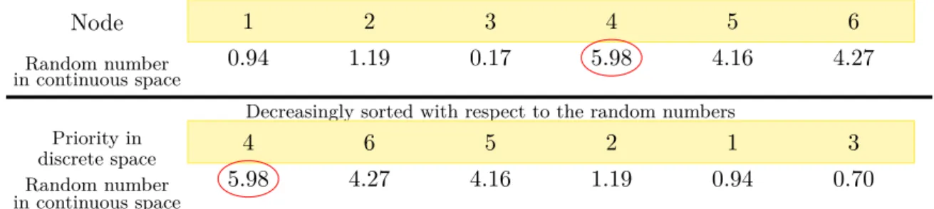
The search space in the solution of the designed CLSC network is discrete, which means that components of each individual from the population cannot have an arbitrary amount, and allowable values are limited only to natural numbers from 1 to N. Hence, the continuous search space has to be changed in WOA algorithm to discrete search space. An example of change in the solution search space is shown in Figure 7.
5
Numerical results
5.1 Sample problems
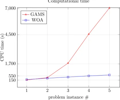
In this section several numerical experiments are generated to validate the developed RFP model and also to assess the performance of the proposed WOA algorithm in terms of the