Using LASSO to Calibrate Non-probability
Samples using Probability Samples
by
Kuang Tsung Chen
A dissertation submitted in partial fulfillment of the requirements for the degree of
Doctor of Philosophy (Survey Methodology) in The University of Michigan
2016
Doctoral Committee:
Professor Michael R. Elliott, Chair Professor Fred M. Feinberg
Probability Samples
N O
N
P
R O
B
A
B I
L I
T
Y
S A M
P L
E S
© Kuang Tsung Chen 2016
ACKNOWLEDGEMENTS
I first would like to express my deepest gratitude to my adviser, Dr. Michael Elliott, for his excellent guidance, patience, and confidence in my ability to complete my research. The trajectory of my life had taken an unexpected yet fulfilling turn more than ten years ago, when Mike offered me a chance to enroll in the post-graduate Biostatistics program at the University of Michigan. While studying in this program, I first met Lucy Huang, a fellow classmate who would later become my wife. And while pursuing my degree in Survey Methodology, our little family has grown from two to four with the births of Aiden and Evelyn, our dearest son and daughter. Mike, you are the ”Moon-Grandpa” in Chinese mythology (like Cupid in classical mythology), who has drawn the fateful connection between my wife and I.
I am grateful to Dr. Rick Valliant, whose casual mention of a research approach has given me the direction for my dissertation. The potential practical application of my research would not have been fully realized in the dissertation, if Dr. Sunghee Lee had not introduced me to an election-polling data. And thanks to Dr. Fred Feinberg, although being a Bayesian at heart, has graciously agreed to read through these frequentist-based materials.
I would not have been able to complete my research without the generous support from the Health and Retirement Study (HRS) at the University of Michigan. I would like to thank its director, David Weir, for giving me an opportunity to work in the HRS while pursuing my degree. And to Mary Beth Ofstedal, the most amazing super-visor a person can hope for, a simple ”thank you” just cannot express this profound
grateful feelings in my heart for you. Your caring friendship, warm understanding, and steadfast support have helped me and my family through some difficult personal as well as professional challenges. You truly are one of the guardian spirits in my life. I am forever indebted to the support I have received from my family throughout the years. To my mother, Shuan-Hwa Chen, who has always been my soul’s spiritual and emotional anchor. To my sister, Victoria Chen, who has taught me the importance of distinguishing between skepticism and cynicism at work and in life. To my mother-in-law, Helen Hsieh, whose boundless energy and love have inspired me to be a better husband and father. To my father-in-law, Ken Huang, for trusting me with your amazing daughter. To aunt Amy Tung, the world’s best baby-sitter, for making it possible for me to focus all my time to complete the final stretch of my dissertation. And last but not least, I would like to thank my wife, Lucy Huang, who is by far the most exuberant and optimistic person I have ever met. Your constant encouragement and unconditional support have given me great strength to continue on our life’s journey. If a man’s fortune is measured by the happiness that surrounds him, you have made me the luckiest person in the world.
TABLE OF CONTENTS
DEDICATION . . . ii
ACKNOWLEDGEMENTS . . . iii
LIST OF FIGURES . . . viii
LIST OF TABLES . . . ix ABSTRACT . . . x CHAPTER I. Introduction . . . 1 1.1 Objective . . . 1 1.2 Non-probability samples . . . 4 1.2.1 Convenience Sampling . . . 5
1.3 Weighting adjustments for non-probability samples . . . 8
1.4 Calibration and model-assisted calibration . . . 10
1.4.1 Traditional calibration . . . 10
1.4.2 Model-assisted calibration . . . 13
1.5 LASSO . . . 15
1.5.1 Definition and notations . . . 16
1.5.2 Oracle property and adaptive LASSO . . . 17
1.6 Outline of chapters . . . 20
II. Calibration with LASSO . . . 22
2.1 Introduction . . . 22
2.2 Calibration . . . 25
2.2.1 Traditional calibration . . . 25
2.2.2 Model-assisted calibration . . . 27
2.3 LASSO . . . 29
2.3.2 Oracle property . . . 29
2.3.3 Determining parameter values and estimates . . . . 31
2.4 LASSO calibration . . . 32
2.4.1 Point estimate: ˆTLASSO y . . . 33
2.4.2 Asymptotic estimator of total . . . 34
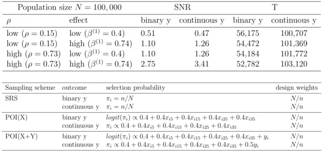
2.4.3 Asymptotic design variance of ˆTLASSO y . . . 38 2.5 Simulation setup . . . 39 2.5.1 Population . . . 41 2.5.2 Sampling schemes . . . 42 2.5.3 Evaluation metrics . . . 44 2.6 Simulation results . . . 45
2.6.1 LASSO relative to ORACLE . . . 46
2.6.2 HT relative to calibration-based estimators . . . 46
2.6.3 LASSO relative to GREG under POI(X) and POI(X+Y) 47 2.6.4 Variance estimates . . . 49
2.7 Application to National Health Interview Survey (NHIS) . . . 59
2.7.1 NHIS and ACS Data . . . 59
2.7.2 Estimators . . . 60
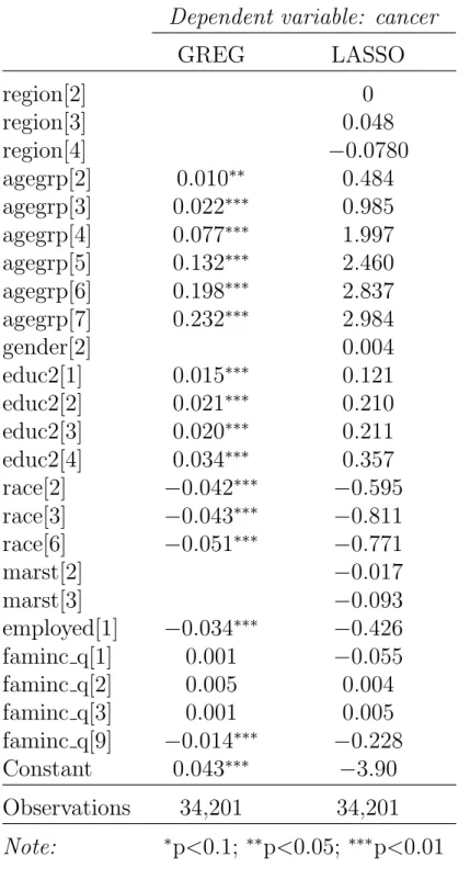
2.7.3 Working models . . . 61
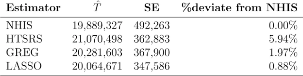
2.7.4 Results . . . 62
2.8 Conclusion . . . 65
III. Calibration with LASSO to Estimated Control . . . 67
3.1 Introduction . . . 67
3.2 Weighting non-probability samples . . . 70
3.2.1 Propensity-score weighting . . . 70
3.2.2 Traditional calibration . . . 72
3.3 Model-assisted calibration . . . 75
3.3.1 Background and notations . . . 75
3.3.2 Assisting model - LASSO . . . 78
3.4 Estimated control LASSO calibration . . . 82
3.4.1 Point estimate: ˆTECLASSO y . . . 83
3.4.2 Asymptotic estimator of total . . . 84
3.4.3 Asymptotic design variance of ˆTECLASSO y . . . 93
3.5 Simulation design . . . 96
3.5.1 Estimators . . . 96
3.5.2 Data and experimental groups . . . 97
3.5.3 Working models . . . 99 3.5.4 Sample generation . . . 101 3.5.5 Evaluation metrics . . . 103 3.6 Simulation results . . . 107 3.6.1 Point estimates . . . 107 3.6.2 Variance estimates . . . 109 3.7 Conclusion . . . 116
IV. Application to Online Political Poll . . . 117 4.1 Introduction . . . 117 4.2 Outcome of interest . . . 119 4.3 Estimation . . . 120 4.4 Weight construction . . . 122 4.4.1 STATEWT . . . 122 4.4.2 PSCORE . . . 124 4.4.3 ECGREG . . . 126 4.4.4 ECLASSO . . . 126 4.5 Variance estimates . . . 128 4.6 Data description . . . 129
4.6.1 Election polling data . . . 129
4.6.2 Analytical sample . . . 130
4.6.3 Benchmark sample . . . 130
4.6.4 Final sample . . . 131
4.7 Variables and working models . . . 131
4.7.1 Variables . . . 131
4.7.2 Working models . . . 133
4.7.3 ECGREG adjusted weights . . . 136
4.8 Results . . . 139
4.8.1 Direction and error . . . 139
4.8.2 Root-mean-square-error . . . 142 4.8.3 Coverage . . . 145 4.9 Discussion . . . 148 4.10 Conclusion . . . 150 V. Conclusion . . . 151 5.1 Summary . . . 151 5.2 Limitations . . . 153 5.3 Future research . . . 155 APPENDICES . . . 157 A.1 Proofs . . . 158
A.1.1 Lemma II.2 . . . 158
A.2 R Code . . . 163
LIST OF FIGURES
Figure
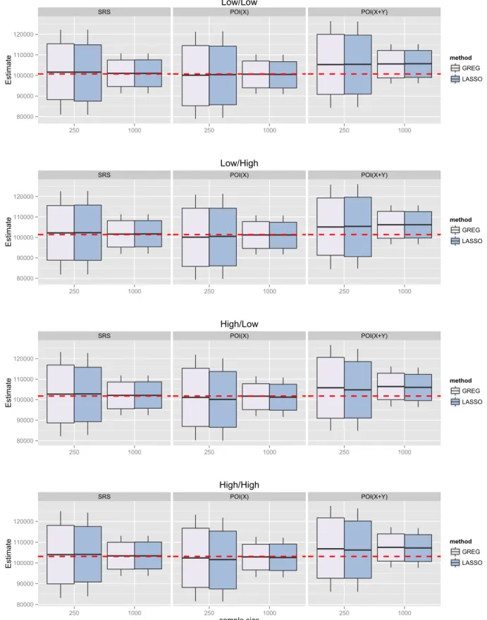
2.1 Boxplot continuous outcome . . . 53
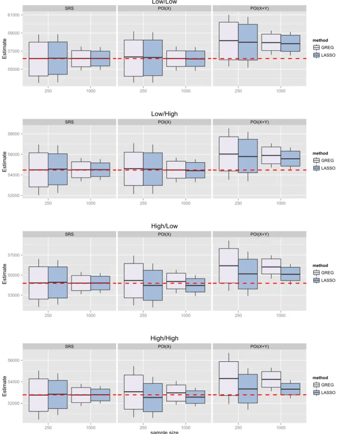
2.2 Boxplot binary outcome . . . 54
3.1 Relative Mean Square Errors . . . 112
4.1 Voting spread for governor race . . . 148
LIST OF TABLES
Table
2.1 Simulation parameters . . . 43
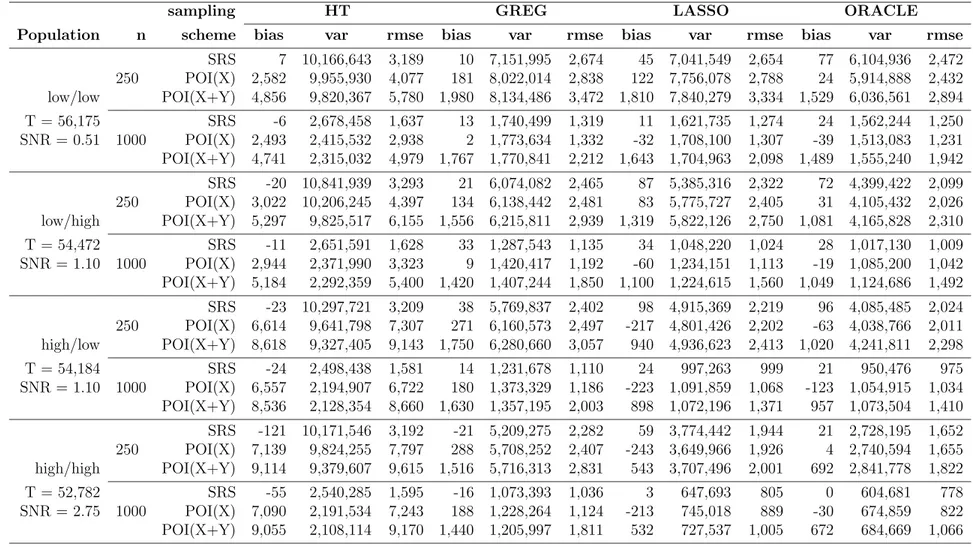
2.2 Simulation summary for continuous outcome . . . 50
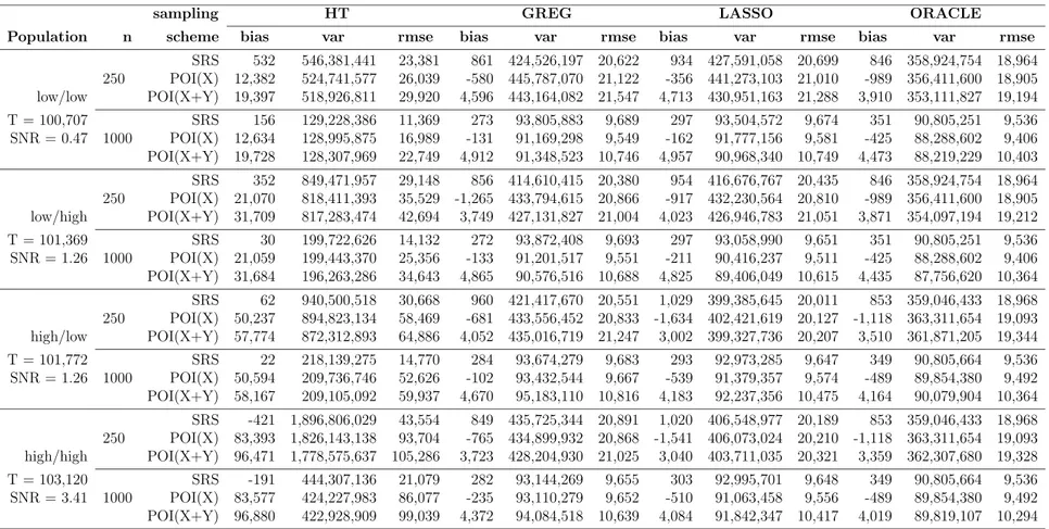
2.3 Simulation summary for binary outcome . . . 51
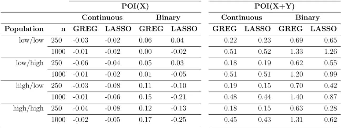
2.4 Bias ratio of LASSO and GREG under POI(X) and POI(X+Y) . . 52
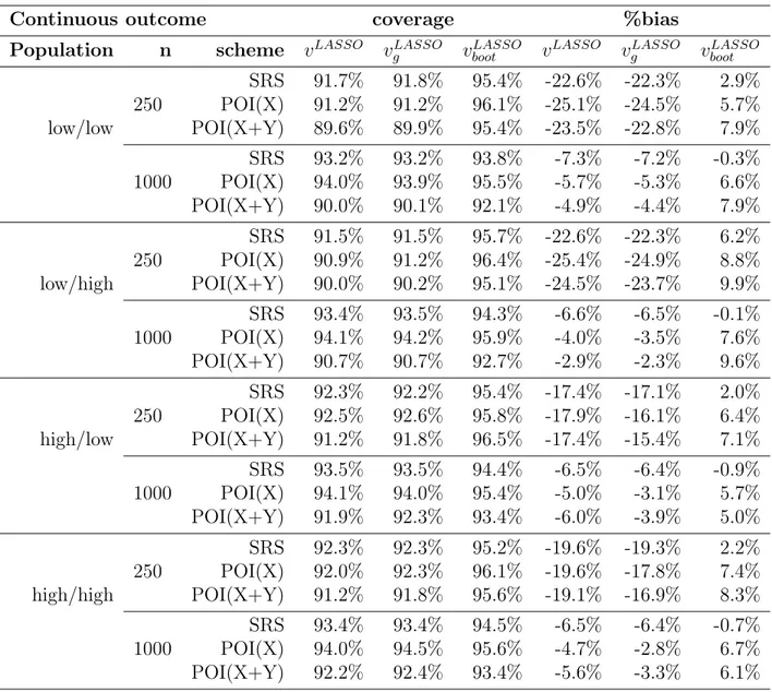
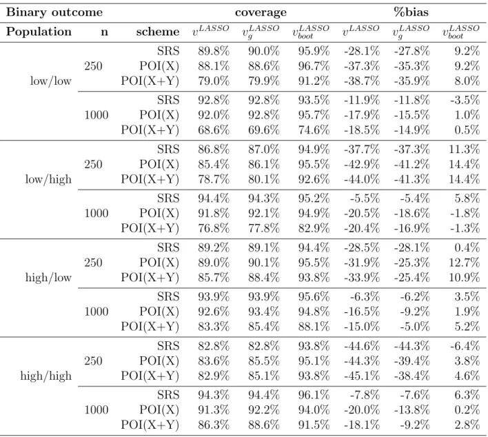
2.5 Relative RMSE of LASSO to GREG under POI(X) and POI(X+Y) 52 2.6 95% nominal coverage and %bias of variance estimates for LASSO . 57 2.7 95% nominal coverage and %bias of variance estimates for LASSO . 58 2.8 Calibration variables . . . 63
2.9 Working model parameter estimates . . . 64
2.10 Results for estimating total number of individuals with cancer . . . 65
3.1 Variables used in the working models . . . 98
3.2 Working models fit on population . . . 102
3.3 Selection probabilities model . . . 104
3.4 Outcome totals by selection probability quintile groups . . . 105
3.5 Simulation parameter summary . . . 105
3.6 Simulation summary . . . 110
3.7 Percentage of times variables are selected by LASSO across 1,000 simulation samples . . . 111
3.8 Variance estimates 95% nominal coverage and %bias . . . 114
3.9 Bootstrap variance estimates and 95% nominal coverage . . . 115
4.1 Governor election covariates and outcome variables . . . 134
4.2 Senate election covariates and outcome variables . . . 135
4.3 U.S. 2014 midterm election governor voting spread estimates and direction . . . 140
4.4 U.S. 2014 midterm election senate voting spread estimates and direction141 4.5 U.S. 2014 governor race RMSE . . . 143
4.6 U.S. 2014 senate race RMSE . . . 144
4.7 U.S. 2014 governor race 90% CI coverage . . . 146
ABSTRACT
Using LASSO to Calibrate Non-probability Samples using Probability Samples by
Kuang Tsung Chen
Chair: Professor Michael R. Elliott
Amidst declining response rates and rapidly increasing costs of probability-based sampling, the resurgence of more cost-effective non-probability sampling has prompted survey researchers to explore different adjustment methods for non-probability sam-ples. The current approach attempts to create one single set of survey weights to correct all imbalances within a non-probability sample. One scheme is to generate estimated selection weights by combining the non-probability sample with a large probability-sampling-based dataset with all variables related to propensity of a re-spondent being in the non-probability sample. In practice, obtaining an appropriate probability sample is costly, and usually there is no way to determine the correct probability of selection for the non-probability sample, or even if all variables are available in the non-probability data to do so. An alternative approach is to adjust the non-probability sample so that the weighted sample totals of a set of variables, known as calibration variables, equal to their Census benchmark totals. Although the method does not require specialized probability-sampling-based data, the result-ing calibrated weights can only correct the imbalance with respect to the limited
of a non-probability sample. To date, no method has shown to be effective in helping researchers make unbiased inference from non-probability samples.
This dissertation addresses the growing demand for making proper inference from non-probability samples. Instead of generating a single set of weights to fix all errors in a non-probability sample, we focus on constructing weights to enable unbiased in-ference for a specific outcome of interest. We introduce the Least Angle Shrinkage and Selection Operator, LASSO, to the framework of model-assisted calibration. The pro-posed method, LASSO calibration, determines the set of variables with the strongest relation to the outcome variable, then calibrates to expected outcome in a probability benchmark sample. The estimator of population total based on LASSO calibrated weights can be unbiased, regardless of how samples are generated. The theoretical framework is developed and evaluated through simulations. An application of LASSO calibration to a large-scale internet-based non-probability sample shows the proposed method can make more accurate and precise inference than existing methods.
CHAPTER I
Introduction
1.1
Objective
Probability-based sampling has dominated survey research for the greater part
of the past century (Stephan, 1948; Frankel and Frankel, 1987). Given complete
measures on sampled units with known selection probabilities, randomization theory removes selection bias by generating representative samples of the target population. On the other hand, non-probability samples that are generated without selection probabilities are automatically at risk for selection bias as samples can easily differ
from the target population on key statistics (Groves, 2006). Well-documented failures
in 1936 and 1948 presidential election polls highlight the potential downfalls in
mak-ing population inference from non-probability samples (Mosteller, 1949). Although
probability-sampling-based framework provides survey practitioners analytical tools to assess and correct sampling errors, declining response rates among all traditional data collection methods — mail, telephone, and face-to-face — are raising concerns
over the potentially high nonresponse bias of probability samples (Curtin et al., 2005;
Holbrook et al., 2007; Groves, 2011; Kohut et al., 2012; Brick and Williams, 2013). Faced with increasing cost to conduct probability-based surveys, many researchers are turning to cheaper and more convenient non-probability sampling methods to achieve
ing will be allocated to online data collection, a platform without a universal sampling
frame to conduct probability-based sampling (Terhanian and Bremer, 2012). With
non-probability sampling quickly on the rise, the demand for practical and effective post-survey adjustment methods of non-probability samples has also increased dra-matically.
Current approach to adjusting non-probability samples is met with limited suc-cess, mainly because researchers attempt to generate one set of sample weights that can work for all variables in the non-probability sample. While the one-size-fit-all is a desirable property of sample weights in public-release surveys, the highly skewed nature of non-probability samples makes it extremely challenging to construct a single set of weights capable of correcting all sample imbalance. This dissertation focuses on making proper inference from a non-probability sample for a specific outcome of
in-terest. We construct weights under the framework of model-assisted calibration (Wu
and Sitter, 2001). The framework uses a model to estimate expected total of the out-come in the population, then calibrates the non-probability sample with respect to the outcome variable. Unlike traditional weighting schemes, model-assisted calibration aims to reduce root-mean-square-error for the weighted estimate of a specific outcome rather than creating a general set of weights that applies to all variables. We employ
the Least Angle Shrinkage and Selection Operator (Tibshirani, 1996), LASSO, as the
assisting model in model-assisted calibration. LASSO performs estimation and vari-able selection simultaneously, which can determine the set of auxiliary information that is most strongly related to the outcome variable to improve calibration weighted estimates for the outcome of interest. The dissertation has two main objectives: (1) Establish the theoretical framework for LASSO calibration in constructing weights
to make inference on a population total, given auxiliary benchmark information on the population.
given a small auxiliary benchmark sample.
We develop and evaluate an estimator based on the LASSO calibrated weights, as well as variance estimation methods for the estimator. We make the following as-sumptions:
(1) There exists a model, ξ, such that the expected value of the outcome variable,
y, can be obtained given a set of covariates X and a vector of parameters β:
Eξ
yi
xi,β = µ(xi,β). Furthermore, the variance of yi is a function of xi or
µ(xi,β): Vξ yi
xi=νiσ2, νi =f(µ(xi,β)) or νi =f(xi).
(2) The full-range of X in the population has non-zero probability of being observed
in the non-probability sample.
Assumption (1) relates the outcome variable to the data through a superpopulation
model ξ. Together with assumption (1), assumption (2) ensures that the model
parameters can be estimated correctly in the non-probability sample because the
relationship betweenyandXcan be fully captured in the sample. If, for example, the
outcome of interest is associated with age 65+, a sample without any respondent age 65+ would violate assumption (2). These two assumptions are the key to successful model-assisted calibration: From the non-probability sample, we can train a model that will accurately predict the expected values of the outcome variable. Then we apply the trained model to a probability-based benchmark sample to recover the distribution of Eξ
h yk
xk,βˆi in the population. Calibrating non-probability sample
yi against population total of Eξ
h yk
xk,βˆi will result in calibrated weights to give unbiased estimate of the outcome. Note that we make no assumption about how non-probability sample respondents participate.
Section 1.2 gives an overview of non-probability samples. Section 1.3 reviews existing post-survey adjustment methods for non-probability samples and their
lim-LASSO regression. Section 1.6 outlines the content for the remaining chapters in the dissertation.
1.2
Non-probability samples
The American Association for Public Opinion Research (AAPOR) categorized non-probability sampling into three broad categories of non-probability sampling:
(1) sample matching, (2) network sampling, and (3) convenience sampling (Couper
et al., 2013). Sample matching is a technique in which respondents are recruited to match characteristics of a target population. A well-known sample matching method is quota sampling, which can produce proper inference if the outcome of interest is associated with quota categories. In 1936 election polls, the Literary Digest collected 2.3 million returned surveys from mostly middle-to-upper income respondents, and predicted the wrong winner with a 17% of error. At the same time, based on a quota sample of 3,000 respondents filling various income by gender quota categories, George Gallup of the American Institute of Public Opinion accurately predicted the winner
with only a 5% of error (Squire, 1988). Quota sampling then was at the forefront
of data collection methods, but did not enjoy the same success in the 1948 election polls. Since then, survey research has shifted to full probability-based sampling.
While sample matching can be viewed as a top-down approach, where desired characteristics of a sample are determined a priori to data collection, network sam-pling takes the bottom-up approach, where a sample starts with an initial set of respondents and gradually builds up through the respondents’ social network given
certain recruitment protocols (Coleman, 1958). An early example of networking
sam-pling is multiplicity samsam-pling (Sirken, 1970), used to enumerate households through
an initial set of household rosters and expanded to households with related members on the rosters. Network sampling also has the potential to collect more data on rare populations than other sampling methods (e.g., an initial H.I.V. positive respondent
can lead to a group of H.I.V. positive patients). It is a popular sampling technique in qualitative sociological research, such as the studies of drug addicts and marijuana
smokers (Lindesmith, 1947; Biernacki and Waldorf, 1981). Given proper conditions
(e.g., random selection of friends in referral procedures, known number of persons connected to a sampled person in their social network), we can draw population inference from network samples based on the theory of respondent-driven sampling (Heckathorn, 1997).
The last type of non-probability sampling, convenience sampling, is probably the most prevalent type of non-probability sampling method in practice. By definition, convenience sampling is a method where “the ease with which potential participants
can be located or recruited is the primary consideration” (Couper et al., 2013). While
survey researchers can determine the types of respondents in quota and, to a lesser extent, network samples, there is little control over the characteristics of respondents in convenience samples. We provide more details on the common types of convenience samples and their potential errors in the following section.
1.2.1 Convenience Sampling
There are four common types of convenience samples in practice.
1. Snowball samples. Snowball sampling starts with a set of participants, then asks them to suggest other people who might be willing to join the study. The sample size grows quickly with each iteration of referrals, like a snowball rolling down the hill. Snowball sampling, while it is sometimes considered as a special type of network sampling, is formally categorized as convenience sampling in this work. The main difference is that, in network sampling, there is a selection and referral policy in place to establish the network, while snowball sampling recruits anyone out of convenience. It is common to observe a snowball sample of respondents with similar characteristics because they share the same
interests, activities, and remain in close contacts. Due to the selective nature of snowball sampling, it is difficult to generalize the results to the population outside of its network. Early sampling literature categorizes snowball sampling
as network sampling, or chain referral sampling (Goodman, 1961; Frank and
Snijders, 1994). We make the subtle point that if the network referral rule is less rigorous and more out of convenience, then the resulting sample is a snowball sample under convenience sampling.
2. Mall intercepts. As the name suggests, mall intercepts are collected at shop-ping centers to gather responses in a short amount of time. At one point, mall-intercept was the second most used data collection method, trailing only
telephone surveys (Nowell and Stanley, 1991). In addition to missing the
cov-erage on the population that does not have access to or go to shopping centers, selection bias can easily occur in mall intercepts when recruiters prefer specific types of shopping malls over others. For example, when recruiters only visit shopping malls at more affluent neighborhoods, measurements on shoppers’ av-erage income and spending can be much higher than those at shopping centers in a low-income neighborhood. Although certain level of probability sampling can be implemented (e.g., selecting shopping centers proportional to size,
ap-proaching everynthperson through the door), the typical goal of mall intercepts
is to collect as many responses as possible with less emphasis (if any) on sample representativeness.
3. River sample. River sampling places survey invitations at designated websites to “intercept” web visitors who are willing to join the study. The method is akin to mall intercept, except the recruitment is carried out online. People who do not have internet access are not covered by river sampling. Since website contents vary greatly to attract readership of different demographics, the choice
of websites to recruit participants can greatly influence sample representation, even more so than the choice of shopping malls in mall intercept. Even if a website generates traffic for all types of web users, there can still be significant selection bias because internet users tend to be younger, more educated, and
with higher income (pewinternet.org, 2015).
4. Volunteer panel. Respondents of volunteer panels actively seek and sign up to participate in a survey or study. Taking the stochastic view of nonresponse (Groves, 2006), we can treat each person as having a propensity to be a volun-teer. From this perspective, the coverage error of volunteer panel is a function of the survey instrument. People without internet access, for instance, can-not volunteer for web surveys. A unique source of error in volunteer panel is self-selection bias. Respondents’ purposeful intent to participate can result in highly skewed measures relative to the general population. For example, people with difficulty sleeping may be much more inclined to participate in a sleep be-havior study. As a result, if sleep duration is an outcome of interest, the sample average hours of sleep can be much shorter than the population’s. While in clinical settings, researchers can recruit from a pool of participants with diverse sleeping patterns, there is no such control in a volunteer sample. A special type of volunteer panel is web volunteer panel. Respondents of web volunteer panel join an online survey company and respond to questionnaires periodically sent out by the survey agency. Researchers in the fields of medicine, sociol-ogy, and psychology have already begun to conduct research with web opt-in
panels (see, for examples, Declercq, Sakala, Corry, and Applebaum, 2007;Butt,
Peipert, Webster, Chen, and Cella, 2013; Popova and Ling, 2014).
While there are many types of non-probability samples, convenience samples are the most prevalent for the obvious reason - they can be obtained the quickest with
tion of convenience samples, making post-survey adjustments of convenience samples particularly challenging. In the following section, we review the common weighting adjustment methods for non-probability samples in practice.
1.3
Weighting adjustments for non-probability samples
The most recent development for adjusting non-probability samples is propensity-score weighting. Propensity-propensity-score adjustment combines the non-probability sample with a probability sample and constructs a propensity model predicting the
proba-bility of a respondent being in the non-probaproba-bility sample (Lee, 2004;Hill and Shaw,
2013). Within the same propensity class, the non-probability sample respondents are matched with probability-selected respondents on all known characteristics that are used in the model. Inverse of the propensity scores serve as pseudo-selection weights for the non-probability sample. For propensity score weights to effectively remove sample bias of an outcome measure, the model covariates must be correlated to both the participation propensity in the non-probability sample and the outcome variable. Large online survey agencies that supply non-probability samples, including Harris Interactive and Toluna, conduct expensive probability-based parallel surveys as refer-ence samples to construct propensity models. Included in their propensity models is a set of “webographic” variables, lifestyle or attitudinal measures that should theoret-ically correlate with both survey measures and respondent participation propensity (Taylor, 2000). These specialized reference surveys have small sample sizes due to high data collection cost, which can result in highly variable propensity-score weights that can inflate variances of the weighted analysis. Furthermore, there are mixed findings on the effectiveness of propensity score adjustments when used as the only
weighting adjustment method. Schonlau et al.(2004) found that propensity score was
more effective at removing bias for categorical variables with two or more categories, but not effective in other types of measures regardless of whether they were factual
or personal. With a longitudinal dataset that allowed for more in-depth analyses of
webographic variables,Schonlau et al.(2009) concluded that propensity-score
weight-ing with webographic variables was effective in reducweight-ing bias in health measures, but not successful for wealth-related variables. The many possibilities of a respondent to participate in non-probability samples present challenges for constructing propensity models. Thus it is common that propensity weights are only successful for a subset of the variables.
To improve propensity-score weighting, Boboth et al. (2007) recommended that
sample calibration, i.e., using weights to “calibrate” samples such that the weighted sample matches the population on key demographic statistics and internet-use, should
always accompany propensity-score adjusted weights. A simulation study by
Beth-lehem (2010) demonstrated that post-stratification, a special case of calibration, was effective in removing selection bias, provided that: (1) the benchmark data is sufficiently large, and (2) the outcome variable is similar for probability and non-probability respondents within the post-stratification cells. The latter case matches the requirements for adjustments of missing at random (MAR) in nonresponse
adjust-ment of probability samples. Through another simulation study, Valliant and Dever
(2011) suggested that such calibration alone can potentially achieve better bias
reduc-tion than propensity-score weighting. We are reminded byValliant and Dever (2011),
however, that if the outcome variable is highly correlated with propensity to be a non-probability sample respondent, no amount of weighting adjustment can completely remove sample bias. This situation falls under not missing at random (NMAR), or non-ignorable nonresponse in the probability framework. For NMAR, only models that strongly predict missing responses under the correct missigness mechanism can improve the analysis.
Both weighting adjustment methods in practice – propensity-score weighting, and calibration to benchmark totals, aim to construct one set of weights such that the
weighted distributions of key statistics in the sample match those in a probability sample or in the population. Many non-probability samples are convenience samples with skewed distributions on many statistics. Thus it is unlikely that one single set of weights can achieve the goal. One major limitation in propensity-score weighting is the quality and size of the probability-based reference sample. It is costly to obtain a large reference sample, and small reference samples can result in unstable propensity weights. Furthermore, there is no systematic way to determine which variables to be included in the propensity models. In calibration weighting, we are limited by the available information on the benchmark data, which can consist of just basic demographics from large-scale government surveys. In that case, variables outside of demographics likely remain skewed. Instead of addressing overall error of the non-probability sample, we focus on improving the inferential property of a specific outcome variable, i.e. bias and variance of a weighted estimate. We choose an alternative approach with calibration, model-assisted calibration, that allows for post-survey adjustment targeting specific outcome of interest. The details of model-assisted calibration are given in the following section.
1.4
Calibration and model-assisted calibration
1.4.1 Traditional calibration
For an analytical sample sA (the sample which requires weight calibration) of
size nA drawn from sample design A, S¨arndal and Deville (1992) defined the term
“calibrated weights”, w
nA×1
, as the adjusted weights that are as close as possible, on
average, to the original design weights, d
nA×1
, with respect to a distance measure
g(wi, di)/qi, under the constraints that wTX =
P
i∈sAwix
T
i = TX, where qi is a
totals of auxiliary variables in X. Formally, wis the solution that minimizes: EA " X i∈sA g(wi, di)/qi # (1.4.1.1)
under the constraint:
X
i∈sA
wixTi =TX (1.4.1.2)
We require that g(wi, di) be differentiable with respect to wi, strictly convex on an
interval containing di (this ensures that the local minimum of the distance function
equals the solution when first derivative is zero), and g(di, di) = 0. The expectation
in equation (1.4.1.1) is taken over sample design A. The most common distance
measure used in practice is the chi-square distance function with qi = 1: g(wi, di) =
(wi−di)2/di. With chi-square distance, letDbe the diagonal matrix of design weights,
the calibrated weights are:
w=d+DX XTDX−1 TX−dTXT (1.4.1.3)
The estimate of population total based on calibrated weights:
ˆ
T =wTy
=dTy+ TX
−dTX XTDX−1XTDy
=dTy+ TX−dTXβˆ (1.4.1.4)
whereβˆis the weighted least square estimate of the linear regression: y=Xβ, given
weights D. Thus there is an implicitly assumed linear relationship between y and
X for traditional calibration. The calibrated weights defined in equation (1.4.1.3) do
variables in the survey. The calibrated weights correspond to generalized regression estimator (GREG) weights, and the weighted total expressed in equation (1.4.1.4)
corresponds to the GREG estimate of total. The linear model, Eξ
yi
xi,β =xT i β,
is referred to as the working model for GREG.
Calibrated weights have four attractive properties: (1) They ensure that for a set of variables in the sample, the sample weighted totals match known population quantities. (2) The weights correct under-coverage of the sub-groups defined by cells
in X. (3) If there are unit non-response in the data, and the missing mechanism is
missing at random (MAR) given X, i.e. respondents and non-respondents with the
same values of X have the same means, then calibrated weights can correct
non-response bias (Kott, 2006). (4) If a survey outcome variable y has a strong linear
relationship with X, then the design-based variance of weighted estimates of y, such
as varA Pi∈s
Awiyi
, is smaller than the design variance with initial design weights,
varA Pi∈s
Adiyi
.
There are also three side-effects from calibration: (1) Weighted estimates based on calibrated weights are no longer unbiased, but they are approximately design unbiased given large population and sample sizes and that the initial design weights
are probability-based. (2) If the relationship between yandX is non-linear, variance
of weighted estimates of y can be larger than the variance of corresponding
pure-design based estimate. (3) The chi-square distance function can lead to negative weights, which do not make sense in many settings.
S¨arndal and Deville (1992) explored a set of distance measures and derived their calibrated weights, for which some are strictly positive. This dissertation focuses on weighted estimates rather than properties of the weights. Thus we focus on calibration
with chi-square distance with qi = 1. Throughout this dissertation, we will compare
our proposed method with estimates from traditional calibration, GREG, since it is widely used in practice. The next section details model-assisted calibration, which
forms the basis of our proposed method.
1.4.2 Model-assisted calibration
In model-assisted calibration (Wu and Sitter, 2001), we assume a relationship
between an outcome y with X through first two moments:
Eξ(yk|xk) = µ(xk,β), Vξ(yk|xk) =νk2σ
2 (1.4.2.1)
whereβ = (β1, . . . , βp)T and σ are unknown superpopulation parameters, µ(xk,β) is
a known function ofxkandβ,νk is a known function ofxkorµ(xk,β). Eξ andVξ are
expectation and variance with respect to the modelξ. LetBbe the finite population
(or census) estimate ofβ (i.e., the quasilikelihood estimator of β based on the entire
finite population), and ˆµi =µ(xi,Bˆ), where ˆB is an estimate ofB based on a sample
of the finite population, the model-assisted calibration weightswminimize a distance
measure: EA " X i∈sA g(wi, di)/qi #
under the constraints:
X i∈sA wi =N X i∈sA wiµˆi = X k∈U ˆ µk (1.4.2.2)
The main conceptual difference between traditional calibration and model-assisted calibration is that in model-assisted calibration, the constraints are based on two
quantities: (1) population total, and (2) population total of predicted values ˆµk.
equation (1.4.1.2)). Define TM = N,P k∈Uµˆk
and M = [d,(ˆµi)i∈sA], under
chi-square distance measure with qi = 1, the model-assisted calibration weights are:
w=d+DM MTDM−1 TM −dTMT (1.4.2.3)
The estimate for population total based on model-assisted calibrated weights are:
ˆ T = (w)Ty =dTy+ TX −dTX XTDX−1XTDy =dTy+ X k∈U ˆ µk− X i∈sA diµˆi ! BM C (1.4.2.4)
where BM C is the calibration slope to satisfy the calibration constraints (different
from the model parameter estimates Bˆ):
BM C = P i∈sAdi(ˆµi−µˆ¯)(yi−y¯) P i∈sAdi(ˆµi−µˆ¯) 2 ˆ¯ µ=X i∈sA diµˆi X i∈sA di ¯ y=X i∈sA diyi X i∈sA di
It is important to note that when the model in equation (1.4.2.1) is linear, i.e.,
Eξ(yk|xk) = xTkβ, then we do not need individual auxiliary xk values from the
pop-ulation. Instead, we can apply Bˆ to the sum of xk in the population to calculate
the constraint in equation (1.4.2.2). Thus when only population totals are available, model-assisted calibration is still possible under a linear model.
When the relationship betweenyandXis closely captured by the superpopulation
model, the resulting calibrated weights are very efficient for estimating a population
re-quiresy, thus model-assisted calibration weights depend on an outcome variable. The weights are constructed specifically to lower the root-mean-square error of weighted
estimates of y, and rely on how well ˆµi approximates the true µi. This dissertation
employs a modern statistical model commonly used in predictive modeling as the
assisting model to capture the relationship between y and X through µ. The
result-ing calibrated weights can improve root-mean-square-error of weighted estimates of
y over traditional calibration estimates. We describe the assisting model in the next
section.
1.5
LASSO
Introduced byTibshirani (1996), LASSO is the acronym for “least absolute
shrink-age and selection operator.” LASSO falls under the general framework of regularized regression, where the solution path to regression coefficients is subject to additional constraints. The early use of mathematical regularization can be found in numerical analysis when solving for a system of equations with more unknowns than the number
of equations (Tikhonov, 1943). There is also a vast literature in image processing and
sound wavelets decoding which apply regularization techniques to filter and de-noise
signals (Donoho and Johnstone, 1994a,b; Abramovich and Benjamini, 1996; Fuchs,
1998; Cand`es et al., 2006; Foucart and Rauhut, 2013). In statistics, the main
ob-jective of regularization is to prevent model over-fitting, so that the same operator (regressors) can produce reliable estimates from different samples of the same
popula-tion (Bickel and Li, 2008). In the past decade, the amount of research on regularized
regression has grown exponentially, driven by the availability of high-dimensional
data in fields such as genetics, medicine, and marketing (see, for examples: Butler
and Denham, 2000; Li, Sung, and Liu, 2007; Goldstein and Osher, 2009; Witten and Tibshirani, 2009; Wang and Zhu, 2010). LASSO regression, in particular, has been widely used as a model selection technique in analyses involving hundreds or
thousands of regressors (Wu et al., 2009; Jagannathan and Ma, 2003), as well as a
predictive model for forecasting (Kamarianakis et al., 2012;Kato and Uemura, 2012).
A wide range of applications and studies have demonstrated that LASSO regression is effective in preventing model over-fitting because it automatically selects more ac-curate and parsimonious models.
The capability of a model trained under a sample to make reliable estimates on a different dataset is a key feature that we need for model-assisted calibration. In the constraint equation of model-assisted calibration, equation (1.4.2.2), the sample predicted values are calibrated against predicted values in the population. If the model is prone to over-fitting in the sample, predicted values in the population would be inaccurate, resulting in unreliable calibrated weights. Thus we employ LASSO as our assisting model as it can simultaneously prevent model over-fitting through variable selection and perform parameter estimation.
1.5.1 Definition and notations
Linear LASSO is a regression of yn×1 onXn×p , where the regression coefficients βp×1 are subject to the constraint:
p−1
X
j=1
|βj| ≤s (1.5.1.1)
The intercept coefficient, β0, is not part of the constraint. Mathematically, linear
LASSO regression coefficients minimize the sum of squares plus the Lagrange multi-plier of the constraint (1.5.1.1):
ˆ β= argmin β X i∈sA yi−xTi β 2 | {z } L +λn p−1 X j=1 |βj| | {z } P (1.5.1.2)
The L term of equation (1.5.1.2) denotes a Loss function, and P is known as the Penalty term. In LASSO, we try to find parameter estimates that minimize the Loss function subject to a penalty. Therefore LASSO is also called a penalized regression
method (Fu, 1998).
Because we are restricting the absolute value of βj (instead of squared or other
powers of βj) in equation (1.5.1.1), LASSO falls under L-1 regularization. When the
penalty isPpj=1−1β2
j instead, it is under L-2 regularization, and the ˆβ is the solution to
the regularized regression known as ridge regression. The parameter λn is a penalty
parameter that optimizes a model-fitness measure (e.g., AIC, BIC), and is often
calculated by cross-validation. The subscriptnemphasizes thatλndepends on sample
size. When sample size is small, λn tends to be large to prevent model over-fitting
by setting coefficients to zero. When sample size is large, there is less chance of
model over-fitting, thus λn tends to 0, and βˆresembles ordinary least square (OLS)
solutions. Since the solution of β in LASSO regression may contain zero(s), LASSO
is also used as a variable selection method. In logistic LASSO (with binary outcome
y), we try to find β that minimizes the negative log-likelihood function:
ˆ β= argmin β X i∈sA [−yix′iβ+ln(1 +exp(−x′iβ))] | {z } L +λn p−1 X j=1 |βj| | {z } P (1.5.1.3)
1.5.2 Oracle property and adaptive LASSO
Suppose the parameters in a full regression model have both zero and non-zero
components, without loss of generality, let the firstp be non-zero and the lastq zero:
βF = β(1)(p×1) β(2)(q×1)=0
The model has the oracle property if it meets the two following criteria (Fan and Li, 2001):
The probability of estimating 0 for zero-valued parameters tends to one:
P rβˆ(2) =0→1.
The estimates of non-zero parameters are as good as if the true sub-model is
known:
√
nβˆ(1)−β(1)→N(0,C)
where C = Σ(β(1)) is the covariance matrix of β(1) under linear model, and C =
I−1(β(1)
) is the inverse of Fisher information matrix of β(1) under generalized linear
model. With the oracle property, a model not only “selects out” zero-valued param-eters by setting them to 0, it also provides accurate estimates to the non-zero model parameters.
While LASSO performs both estimation and variable selection, it has been shown that in order for LASSO to have the oracle property, the regression design matrix has
to satisfy fairly strict conditions, called “Irrepresentable Condition” (Zhao and Yu,
2006). The condition requires that covariates corresponding to the zero components of the regression parameters not contributing meaningfully to the estimation of the non-zero parameters. An example of a regression matrix satisfying irrepresentable
condition is a matrix where the correlation between covariates are constant r, and
there exists a constant c > 0 such that 0 < r ≤ 1/(1 +cq), where q is the number of zero-valued parameters. In practice, data gathered from surveys seldom have a set of covariates with well-defined structures to satisfy irrepresentatble condition. Thus from model consistency point view, LASSO is not practical in survey research.
specified models, even without the irrepresentable condition (Zhao and Yu, 2006). The adaptive LASSO regression coefficients are obtained by adding a weight param-eter, αj, to the penalty term:
ˆ β =argmin β X i∈sA yi−xTi β 2 +λn p X j=1 αγj |βj| ! (1.5.2.1)
Similarly for adaptive logistic LASSO:
ˆ β=argmin β X i∈sA −yi xTi β +log 1 +exp xTi β +λn p X j=1 αγj |βj| ! (1.5.2.2)
The role of the weight parameter, αj, is to prevent LASSO from selecting covariates
with large effect sizes in favor of lowering prediction error when the sample size is small. Thus the weights are inversely proportional to effect sizes of regression
parameters: αj ∝ 1 |βj|. Common choices of αj: αj = 1 βˆjM LE , where ˆβjM LE is
the maximum likelihood estimate of βj, or αj = 1 βˆjRIDGE
, where ˆβjRIDGE is the
ridge regression estimates ofβj mentioned in Section 1.5.
The power of the weight parameter, γ, is a constant greater than 0 that interacts
with αj to control LASSO from selecting or excluding parameters. For example, if
we still want LASSO to favor large effect covariates when the sample size is small, we
should set γ small. If we want to de-emphasize effect sizes further, we should set γ
large. Zou (2006) has shown that the oracle property is satisfied only when:
λn √ n/(√n)γ → ∞ and λn √ n→0
The conditions require thatλn grow at least at the rate of √n
(√n)γ, but not faster
than √n. In practice, we do not observe the theoretical rate of growth ofλn, unless
a large number of samples with different sample sizes are collected from the same
implementation (Friedman et al., 2010), a range ofλn is determined by the following
scheme:
(1) Set γ = 0.
(2) Determine λmax
n by finding the smallestλn that sets all coefficients to 0.
(3) If sample size n is larger than the number of parameters in the regression model,
setλmin
n = 0.0001λmaxn . If sample sizenis smaller than the number of parameters,
set λmin
n = 0.01λmaxn (to set parameters to 0 sooner).
(4) Generate a grid ofλn, typically 100 equally spaced points betweenλminn andλmaxn .
The initial range of values of λn is determined independently of γ. With an
ini-tial range of values of λn, a modeler can use data-driven techniques, such as
cross-validation, to find λn given a γ. Choices of γ are less data-driven. Some modelers
choose one of γ = 0.1,0.5,1,2. We can also perform cross-validation for each pair
of (λn, γ), given a model-fitness metric (e.g. mean-absolute-error, area under curve,
etc.).
1.6
Outline of chapters
The organization of the dissertation is as follows: Chapter II establishes the the-oretical framework for LASSO-assisted calibration, given population auxiliary data. We derive the estimator of population total with LASSO calibrated weights, and asymptotic expectation and variance estimators for the total. The estimator and variance estimates are evaluated through simulation under different types of popula-tions and sampling schemes. The root-mean-square of the estimator is compared with an unadjusted estimator as well as traditional calibration estimator of totals for both continuous and binary outcome variables. In Chapter III, we extend LASSO calibra-tion to cases where the benchmark data is a probability-based sample. We introduce
the estimated-control LASSO calibration estimator, ECLASSO, to estimate popula-tion totals. Asymptotic expectapopula-tion and variance estimates are derived. We evaluate ECLASSO under simulation with National Health Interview Survey 2013 data as the population, given different levels of sample and benchmark sizes. The root-mean-square error of ECLASSO is compared to traditional calibration estimator, GREG, estimated-control generalized regression estimator, ECGREG, and the propensity-score weighted estimates of total, PSCORE. In Chapter IV, we apply ECLASSO to an actual non-probability internet-based election polling data. Given the actual elec-tion results, we compare root-mean-square error of elecelec-tion forecasts by unweighted estimate, UNWT, ECLASSO, ECGREG, and PSCORE. The final chapter, Chapter V, provides the summary, implications, and limitations of current research, as well as potential extensions for future research.
CHAPTER II
Calibration with LASSO
2.1
Introduction
For many survey agencies, adjusting survey weights to known auxiliary
informa-tion is the final and most crucial step in the weight construcinforma-tion process. S¨arndal and
Deville (1992) introduced the term “calibrated weights” as the adjusted weights that are as close as possible to the original design weights while adhering to a set of con-straints. The constraints are known population totals for a set of auxiliary variables in the survey. The calibrated weights ensure that the weighted sum of each auxil-iary variable equals to its corresponding total in the population. Calibration plays an important role in official statistics because it can generate weights such that the weighted demographic estimates across different surveys are consistent. Examples of large-scale surveys producing calibrated weights include Consumer Expenditure
Survey (Jayasuriya and Valiant, 1996), Canadian Labour Force Survey (Singh et al.,
2001), and Survey of Health Aging and Retirement in Europe (B¨orsch-Supan et al.,
2013).
In probability samples, when design weights equal to the inverse of selection prob-abilities, weighted estimates of totals are design-unbiased for the population total. A main objective of calibration is to correct sample undercoverage by adjusting
sub-calibrated weights can be applied to all variables in the survey, because they main-tain the unbiased property of original design weights. In non-probability samples, however, there are no selection probabilities to construct initial design weights that can produce unbiased estimates. Thus there is no guarantee that the traditional cal-ibrated weights can work for all variables in the non-probability sample. To make inference from non-probability samples, one practical approach is to construct a set of weights that can lower the root-mean-square error (RMSE) of weighted estimates with respect to a specific outcome of interest. Model-assisted calibration provides the framework to construct calibrated weights targeting an outcome variable, given
a model that can approximate the expected values of the outcome (Wu and Sitter,
2001). The key to successful model-assisted calibration is a model with strong predic-tive properties: model parameters estimated from one sample can be used to reliably predict values in a different sample of the same population.
The Least Angle Shrinkage and Selection Operator, LASSO, is a regularized
re-gression that can perform both variable selection and parameter estimation (
Tibshi-rani, 1996). Kamarianakis et al. (2012) found success with LASSO in predicting
average traffic speed in the presence of severe multi-collinearity due to aggregated
area-level regressors. Kato and Uemura (2012) applied LASSO to predict the signal
of a star being observable in the sky, given a large set of periodic amplitude val-ues. The non-signal amplitudes are considered as noise, and LASSO was successful in filtering out noise to detect the true signal. In the fields of genetics and finance, LASSO is also used in prediction modeling given hundreds or thousands of
predic-tors (Wu et al., 2009; Wang and Zhu, 2010). A wide range of applications have
demonstrated that LASSO is effective in preventing model over-fitting by automat-ically selecting more accurate and parsimonious models. In survey research, under
traditional calibration, McConville (2011) has developed the theoretical framework
esti-mator of total for a continuous outcome variable, given LASSO regression parameter
estimates. More recently, McConville et al. (2015) examined the use of LASSO
un-der the model-assisted calibration framework in a simulation study that can extend LASSO calibration to estimating totals of non-continuous outcomes, and showed em-pirically (not theoretically) that model-assisted LASSO calibration can result in much smaller RMSE than traditional calibration. Although model-assisted calibration with LASSO holds great promise in constructing a set of weights that can result in small RMSE of weighted estimates for an outcome variable in a non-probability sample, there is no theoretical framework established for the bias and consistency properties of model-assisted LASSO calibration estimators. The main objectives of this chapter are:
(1) Develop the theoretical framework for model-assisted calibration with LASSO for both continuous and binary outcome variables: derive the point estimate of total, its asymptotic expectation, and asymptotic theoretical variance estimate.
(2) Investigate relative performances, in terms of root-mean-square-error, of LASSO calibration to traditional calibration under different outcome types, sampling schemes, sample sizes, and calibration variable covariance structures. The aim is to understand the situations where LASSO calibration can work well.
The framework for non-probability-based sampling is equivalent, except we as-sume the initial design weights are obtained under simple-random-sampling (SRS) regardless of how the samples are formed. The theoretical framework of LASSO cal-ibration allows for estimating population totals from a non-probability sample with small root-mean-square-error. When the outcome of interest is binary, the LASSO calibration estimator of the total can have large gains in RMSE relative to traditional calibration estimator of the total, because traditional calibration assumes a linear relationship between the outcome and calibrated auxiliary variables. Many variants
of LASSO have been developed since LASSO’s introduction nearly two decades ago.
The adaptive LASSO (Zou, 2006), in particular, has shown to have model-consistency
properties, i.e., selecting the correct variables and providing unbiased estimates of pa-rameters under mild conditions. Thus we employ the adaptive LASSO as the assisting model in model-assisted calibration. To simplify naming, we refer to adaptive LASSO simply as LASSO for the remainder of this chapter.
The organization of the chapter is as follows: Sections 2.2 and 2.3 provide the definition and notations of calibration and LASSO regression. Section 2.4 develops the LASSO calibration estimator of population total, its asymptotic estimator, and asymptotic variances. Sections 2.5 and 2.6 describes the simulation and results for
evaluating the root-mean-square-error and variance estimates of ˆTLASSO
y . The chapter
ends with Section 2.8 summarizing the findings.
2.2
Calibration
2.2.1 Traditional calibration
For an analytical sample sA (the sample which requires weight calibration) of size
nA drawn from sample design A with design weights d
nA×1
, and the diagonal matrix
of design weights D, calibrated weights w
nA×1
minimize a distance measure:
EA " X i∈sA g(wi, di)/qi # (2.2.1.1)
under the constraint:
X
i∈sA
wixTi =TX (2.2.1.2)
weight di. We focus on the most common distance measure used, the chi-square
distance: g(wi, di) = (wi−di)2/di with qi = 1. Under this distance measure:
wGREG =d+DX XTDX−1 TX−dTXT (2.2.1.3)
where TX is a row vector of known population totals of sample calibration variables
X. The estimate of population total of outcome y based on calibrated weights:
ˆ TyGREG =w T y =dTy+ TX −dTX XTDX−1XTDy =dTy+ TX−dTXβˆ (2.2.1.4)
where βˆ = XTDX−1XTDy is the weighted least square estimate of the linear
regression y = Xβ, given weights D. The calibrated weights defined in equation
(2.2.1.3) do not rely on any outcome variable. Thus the same set of weights can be applied to all variables in the survey. The weighted total expressed in equation (2.2.1.4) corresponds to the generalized regression estimator (GREG) of total, thus
we denote the weightswGREG and the estimator ˆTGREG
y . In GREG, an implicit linear
relationship is assumed. The linear model, Eyi
xi,β = xT
i β, is referred to as the
working model for GREG. Although ˆTGREG
y is asymptotically design-unbiased for
Ty, when the relationship between y and X is non-linear, such as in the case when
y is binary, the variance of ˆTGREG
y can be larger than the variance of pure-design
based estimator of total (an estimator not using auxiliary totals). Model-assisted
calibration estimators can have significant advantage over ˆTGREG
y in reducing variance
of estimates of totals, because model-assisted calibration allows for non-linear models to assist in the construction of calibrated weights. In the next section, we briefly describe the framework for model-assisted calibration.
2.2.2 Model-assisted calibration
In model-assisted calibration, we assume a relationship between an outcome y
and X through first two moments (Wu and Sitter, 2001):
Eξ(yk|xk) = µ(xk,β), Vξ(yk|xk) =νk2σ
2 (2.2.2.1)
whereβ = (β1, . . . , βp)T and σ are unknown superpopulation parameters, µ(xk,β) is
a known function ofxkandβ,νk is a known function ofxkorµ(xk,β). Eξ andVξ are
expectation and variance with respect to the modelξ. LetBbe the finite population
(or census) estimate ofβ (i.e., the quasilikelihood estimator of β based on the entire
finite population), and ˆµi =µ(xi,Bˆ). The model-assisted calibrated weights w then
minimize a distance measure:
EA " X i∈sA g(wi, di)/qi #
under the constraints:
X i∈sA wi =N X i∈sA wiµˆi = N X k=1 ˆ µk (2.2.2.2)
The main conceptual difference between traditional calibration and model-assisted calibration is that in model-assisted calibration, the constraints are based on two
quantities: (1) population total, and (2) population total of predicted values ˆµk.
In traditional calibration, the constraint is a vector of population totals of X (see
model-assisted calibrated weights are: wM C =d+DM MTDM−1 TM −dTMT (2.2.2.3) where TM = hN,PN k=1µˆk i
and M = [d,(ˆµi)i∈sA]. The estimate for the population
total based on model-assisted calibrated weights is then:
ˆ TyM C = w M CT y =dTy+ TX −dTX XTDX−1XTDy =dTy+ N X k=1 ˆ µk− X i∈sA diµˆi ! ˆ BM C (2.2.2.4)
where ˆBM C is the calibration slope to satisfy the calibration constraints (different
from the model parameter estimates Bˆ):
ˆ BM C = P i∈sAdi(ˆµi−µˆ¯)(yi−y¯) P i∈sAdi(ˆµi−µˆ¯) 2 ˆ¯ µ=X i∈sA diµˆi X i∈sA di ¯ y=X i∈sA diyi X i∈sA di
Unbiasedness and small variances of ˆTM C
y both rely on how well the ˆµi approximates
2.3
LASSO
2.3.1 Definition and parameters
The adaptive LASSO regression coefficients are obtained by solving a penalized
regression equation. For linear adaptive LASSO regression (Zou, 2006):
ˆ β =argmin β X i∈sA yi−xTi β 2 +λn p X j=1 αγj |βj| ! (2.3.1.1)
Similarly for logistic adaptive LASSO:
ˆ β=argmin β X i∈sA −yi xTi β +log 1 +exp xT i β +λn p X j=1 αγj |βj| ! (2.3.1.2)
Given λn and γ, we can calculate βˆ through some iterative procedures.
The role of the weight parameter, αj, is to prevent LASSO from selecting
co-variates with large effect sizes in favor of lowering prediction error when the sample size is small. Thus the weights are inversely proportional to effect sizes of regression
parameters: αj ∝ 1 |βj|. A common choice of αj: αj = 1 βˆjM LE , where ˆβjM LE
is the maximum likelihood estimate of βj. The power of the weight parameter, γ,
is a constant greater than 0 that interacts with αj to control LASSO from
select-ing or excludselect-ing parameters. For example, if we still want LASSO to favor large
effect covariates when the sample size is small, we should set γ small. If we want to
de-emphasize effect sizes further, we should set γ large.
2.3.2 Oracle property
An important concept in measuring the performance of a model selection and estimation method is called the “oracle property”. The optimal method selects the correct variables and provides unbiased estimates to selected parameters. Suppose the parameters in a full regression model have both zero and non-zero components,
without loss of generality, let the first p be non-zero and the lastq zero: βF = β(1)(p×1) β(2)(q×1) =0
A regression model has the oracle property if it satisfies the following conditions Fan
and Li (2001):
The probability of estimating 0 for zero-valued parameters tends to one:
P rβˆ(2) =0→1.
The estimates of non-zero parameters are as good as if the true sub-model is
known:
√
nβˆ(1)−β(1)
→N(0,C)
where C = Σ(β(1)) is the covariance matrix of β(1) under linear model, and C =
I−1(β(1)
) is the inverse of Fisher information matrix of β(1) under generalized linear
model. For finite-population inference, suppose ν indexes a population with size Nν,
let B be the quasilikelihood estimates of β in population ν, and Bˆ is the estimate of
Bbased on a sample with size nν ≤Nν, the finite-population equivalent of the oracle
property is: P rBˆ(2) =0→1 √n ν ˆ B(1)−B(1)→N ν(0,Cν) B →β as ν → ∞
where Cν = Σ(B(1)) is the covariance matrix of B(1) under linear model, and C =
model. For convenience, we omit ν from the notations. It is assumed that N and n
are sequences of numbers, both grow to infinity asν → ∞. We writeB→βto mean
that B approaches β as both sample and population sizes grow.
Zou (2006) has shown that if:
λn
√
n/(√n)γ → ∞ and λn
√ n→0
then the adaptive LASSO satisfies the oracle property. The conditions require that
λn grow at least at the rate of √n
(√n)γ, but not faster than √n. We discuss the
choice of λn and γ in the next section.
2.3.3 Determining parameter values and estimates
In practice, we do not observe the theoretical rate of growth ofλn, unless we have
obtained many samples of the same population with various sample sizes. Given a
sample, the choices ofλn andγ depend on the modeler. In Rglmnetimplementation
(Friedman et al., 2010), a range of λn is determined by the following scheme:
(1) Set γ = 0.
(2) Determine λmax
n by finding the smallestλn that sets all coefficients to 0.
(3) If sample size n is larger than the number of parameters in the regression model,
setλmin
n = 0.0001λmaxn . If sample sizenis smaller than the number of parameters,
set λmin
n = 0.01λmaxn (to set parameters to 0 sooner).
(4) Generate a grid ofλn, typically 100 equally spaced points betweenλminn andλmaxn .
The initial range of values of λn is determined independently of γ. Choices of γ is
less data-driven. Some modelers choose one of γ = 0.1,0.5,1,2. In this chapter, we determine (λn, γ) through cross-validation as follows:
Step 1. Obtainαj = 1 βˆjM LE
Step 2. Determine 100 equally spaced values ofλn based on R glmnet’s
implemen-tation.
Step 3. For each pair (λn, γ),λn from Step 2, andγ = 0.1,0.5,1,2, split data into 5
folds. Use 4 folds to obtain βˆ.
Step 4. Applyβˆto the last fold not used to estimate βˆand calculate a metric. For
continuousy, we calculate the mean-absolute-error (MAE),Pi∈s
A(k)|µˆi−yi|.
For binary y, we calculate the area under curve (AUC) (calculated through
Rglmnet::auc function).
Step 5. Average the 5 metrics for each pair of (λn, γ), and choose the pair with the
best average metric: minimum MAE for continuous y, maximum AUC for
binary y.
The adaptive LASSO coefficient estimates are then obtained by solving (2.3.1.1) or
(2.3.1.2) given the selected (λn, γ). The R code used to perform cross-validation in
this dissertation is in Appendix A.2.
2.4
LASSO calibration
This section develops the main theoretical framework of this chapter. We derive the analytical formula for LASSO estimator of total, its asymptotic expectation, and asymptotic linearized variance estimates. We make the following assumptions in the theoretical framework:
A. The samples are drawn from a single-stage sample design A, allowing for unequal
probabilities of selection. The selection probability for unit i is denoted by πA
i ,
and the joint selection probability of units i and j is denoted byπA
the design weight for unit i by dA
i = 1/πiA, the vector of design weights by dA,
and the diagonal matrix of design weights by DA.
B. Population-level auxiliary data are known, denoted by X= (xT
k), k= 1,· · ·, N.
C. A superpopulation model is assumed, as is described in section 2.3.3:
Eξ(yi|xi) =µ(xi,β)
Vξ(yi|xi) =νi2σ2
D. The true superpopulation parameters are a subset of the full regression model
for LASSO: βF = β(p×1) β(2)(q×1)
E. The full-range of Xin the population has non-zero probability of being observed
in the analytical sample.
2.4.1 Point estimate: TˆLASSO
y
The LASSO calibration estimate of total can be obtained following the steps:
Step 1. Obtain LASSO regression coefficients Bˆ as described in section 2.3. We
use R packageglmnet (Friedman et al., 2010) to obtain LASSO coefficients
for both linear and glm models, given a pair of (λn, γ) selected by
cross-validation. Linear LASSO:
ˆ B=argmin β X i∈sA yi−xTi β 2 +λn p X j=1 αjγ|βj| ! Logistic LASSO: ˆ B=argmin β X i∈s −yi xTi β +log 1 +exp xT i β +λn p X j=1 αγj |βj| !
Step 2. UseBˆ to calculate ˆµi =µ(xi,Bˆ) in the sample and the population. Step 3. Define TM = N,PN k=1µˆ and M = dA,(ˆµ i)i∈sA
, under chi-square
dis-tance measure with qi = 1:
wLASSO=dA+DAM MTDAM−1 TM −(dA)TMT (2.4.1.1)
Step 4. LASSO calibration estimator of total:
ˆ TLASSO y = w LASSOT y = (dA)Ty+ TX−(dA)TX XTDAX−1XTDAy = (dA)Ty+ N X k=1 ˆ µk− X i∈sA dAi µˆi ! ˆ BM C (2.4.1.2)
where ˆBM C is the calibration slope to satisfy the calibration constraints
(different from the model parameter estimates Bˆ):
ˆ BM C = P i∈sAd A i (ˆµi−µˆ¯)(yi−y¯) P i∈sAd A i (ˆµi−µˆ¯)2 ˆ¯ µ= X i∈sA dA i µˆi X i∈sA dA i ¯ y= X i∈sA dAi yi X i∈sA dAi
2.4.2 Asymptotic estimator of total
Wu and Sitter (2001) established the conditions to derive asymptotic model-assisted calibration estimator. We state the conditions here with slight
modifica-tion in notamodifica-tions to be consistent with the current research. Let β be the true
superpopulation parameter for the model defined in equation (2.2.2.1), andB be the
deriving LASSO calibration asymptotic estimator of total:
(2.4.2.i) Bˆ = B + Op(1/√n), B is the finite-population regression slope of β,
B →β.
(2.4.2.ii) For each xi, ∂µ(xi,t)/∂t is continuous in t, and maxi|∂µ(xi,t)/∂t| ≤
h(xi,β) for t in a neighborhood of β, and N−1
P
i∈Uh(xi,β) =O(1).
(2.4.2.iii) For eachxi,∂2µ(xi,t)/∂t∂tT is continuous int, andmaxj,k|∂2µ(xi,t)/∂tj∂tk| ≤
k(xi,β) fort in a neighborhood of β, and N−1
P
i∈Uk(xi,β) =O(1).
(2.4.2.iv) The Horvitz-Thompson estimators of certain population means are
asymp-totically normally distributed.
(2.4.2.v) λn (√n/(√n)γ) → ∞ and λn √ n→0.
Remark II.1. The certain means in condition (2.4.2.iv) are means of first and second derivatives of µ(xi,t) in the Taylor series expansion ofµ(xi,t) evaluated at a
neigh-borhood aroundB, which is a vector of values ifBhas more than one parameter. The
condition requires that the Horvitz-Thompson estimates of the means are bounded element-wise.
Lemma II.2. Assume the superpopulation model:
Eξ(yk|xk) = µ(xk,β), Vξ(yk|xk) =νk2σ2
LetBbe the finite-population quasilikelihood estimate ofβ,B →β. Under conditions (2.4.2.i)-(2.4.2.vi), the model-assisted asymptotic estimator of population total is:
ˆ TM C y = X i∈sA dA i (yi−µiBM C) + N X i=1 µiBM C+op N √n (2.4.2.1)