Total activation: fMRI deconvolution through spatio-temporal regularization

(1)

Total activation: fMRI deconvolution through spatio-temporal regularization

Fikret I

_şı

k Karahano

_ğ

lu

a,b,

⁎

_{, César Caballero-Gaudes}

b,c

_{, François Lazeyras}

b

_{, Dimitri Van De Ville}

a,b a

Institute of Bioengineering, Ecole Polytechnique Fédérale de Lausanne (EPFL), Switzerland b

Department of Radiology and Medical Informatics, University of Geneva, Switzerland c_{Basque Center on Cognition, Brain and Language, Donostia-San Sebastian, Spain}

a b s t r a c t

a r t i c l e i n f o

Article history:

Accepted 22 January 2013 Available online 4 February 2013 Keywords: fMRI BOLD Deconvolution Sparsity Total variation Spatio-temporal regularization Paradigm-free mapping Resting state

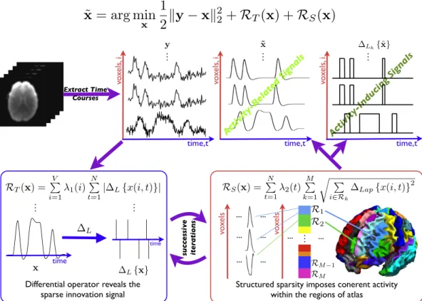
Conﬁrmatory approaches to fMRI data analysis look for evidence for the presence of pre-deﬁned regressors modeling contributions to the voxel time series, including the BOLD response following neuronal activation. As more complicated questions arise about brain function, such as spontaneous and resting-state activity, new methodologies are required. We propose total activation (TA) as a novel fMRI data analysis method to explore the underlying activity-inducing signal of the BOLD signal without any timing information that is based on sparse spatio-temporal priors and characterization of the hemodynamic system. Within a variation-al framework, we formulate a convex cost function—including spatial and temporal regularization terms—

that is solved by fast iterative shrinkage algorithms. The temporal regularization expresses that the activity-inducing signal is block-type without restrictions on the timing nor duration. The spatial regulariza-tion favors coherent activaregulariza-tion patterns in anatomically-deﬁned brain regions.

TA is evaluated using a software phantom and an event-related fMRI experiment with prolonged resting state periods disturbed by visual stimuli. The results illustrate that both block-type and spike-type activities can be recovered successfully without prior knowledge of the experimental paradigm. Further processing using hierarchical clustering shows that the activity-inducing signals revealed by TA contain information about meaningful task-related and resting-state networks, demonstrating good abilities for the study of non-stationary dynamics of brain activity.

Introduction

Conventional analysis of functional magnetic resonance imaging (fMRI) data heavily relies on approaches based on general linear models (GLMs) where prior knowledge about the experimental paradigm; i.e., onsets and durations of stimuli, is used to construct tempo-ral regressors, which are thenfitted to the time course of every voxel. The subsequent statistical hypothesis testing, for a given contrast of_fitted weights, is a mass univariate approach leading to an“activation map” that highlights brain regions for which sufficient evidence is present to be related to the experimental paradigm. The relationship between the measured blood oxygen level dependent (BOLD) and the experimental paradigm can be modeled as a linear shift-invariant system with the he-modynamic response function (HRF) as an impulse response. In standard GLM approached (Friston et al., 1998), the HRF is predefined using gamma functions; moreflexible techniques estimate HRF components in a subject- or time-dependent way in order to deal with inter- and intra-subject variability (Aguirre et al., 1998). More notably,

parcel-based HRF estimation methods through joint detection estimation (JDE) framework are studied based on Bayesian approaches (Chaari et al.,

2013; Makni et al., 2008; Vincent et al., 2010). Recently, an adaptive parcel

identiﬁcation driven by the hemodynamics is proposed using JDE (Chaari

et al., 2012; Thirion et al., 2006). These HRF identiﬁcation methods are

mainly combined with GLM analysis to explore the parcel/subject/ group/task speciﬁc hemodynamic models.

Not all brain activity can be modeled beforehand using stimulus functions; e.g., interictal epileptic discharges occur spontaneously. In addition, mere resting-state, which was neglected before as back-ground noise, is known (Raichle, 2006) to produce characteristic patterns of brain activity referred to as resting-state networks. Such unpredictable activity cannot be inferred from traditional GLM analy-sis approaches (Gusnard and Raichle, 2001). Therefore, there is an increasing need for methodologies that enable the exploration of hemodynamic brain activity without predeﬁned responses (Cole et

al., 2010). Data-driven methods have been proposed for that purpose

such as fuzzy clustering (Baumgartner et al., 2000), temporal cluster-ing analysis (TCA) (Liu et al., 2000; Morgan et al., 2008), seed correla-tion analysis (Biswal et al., 1995), or subspace decomposition methods such as independent component analysis (ICA) (Beckmann

and Smith, 2004; Calhoun and Adali, 2006), canonical correlation

analysis (CCA) (Afshin-Pour et al., 2012) and agnostic canonical vari-ates analysis (agnostic-CVA) (Evans et al., 2010). ICA is probably the

⁎ Corresponding author at: Institute of Bioengineering, Ecole Polytechnique Fédérale de Lausanne (EPFL), Switzerland.

Contents lists available atSciVerse ScienceDirect

NeuroImage

(2)

most commonly used data-driven method. It provides a bilinear decom-position of the data into components that consist out of a spatial map with an associated time course. Its application to fMRI typically relies on (a surrogate for) spatial statistical independence between the com-ponents. However, such criterion is not directed speciﬁcally to identify “activation like_”components since no knowledge is taken into account about the hemodynamics or about the type of activity-driven signal (e.g., spikes versus sustained activity).

fMRI deconvolution methods have been proposed to uncover the underlying activity-inducing signal at the fMRI timescale of seconds. Initially,Glover (1999)introduced Wiener deconvolutionﬁltering that is optimal for Gaussian sources and thus results in very smooth activity-inducing signals. This work was generalized byGitelman et

al. (2003)to study the psychophysiologic interactions at the

neuro-nal level. Following recent advances in convex optimization theory, these methods can be made more sophisticated by adding sparse priors on the underlying signal and solve maximum a posteriori estimation rather than naive maximum likelihood estimation. They have been exploited as an extension to standard GLM analysis by deﬁning spatial priors on spatial activation maps (Flandin and Penny, 2007; Harrison et al., 2008; Smith and Fahrmeir, 2007;

Vincent et al., 2010). Within a temporal fMRI deconvolution

framework, while the linear system assumption on the hemodynam-ic model is retained, regularization terms use‘1-norm to favor sparse solutions in time; i.e., a limited number of spike-like activations. For

example, Hernandez-Garcia and Ulfarsson (2011) use the

majorization–minimization scheme,Gaudes et al. (2011, 2013)rely on ridge-regression and sparsity-promoting estimators, and

(Khalidov et al., 2007, 2011) impose sparsity in the

activelet-domain, a wavelet basis that is tailored to the hemodynamic proper-ties. These methods do not require any knowledge on the timing and exploit temporal properties of the HRF. Promising results have been demonstrated for local event detection (Gaudes et al., 2011), espe-cially in epilepsy (Lopes et al., 2012), but also for resting-state anal-ysis (Petridou et al., 2012). Recently, non-linear models have also attracted a lot of attention for blind deconvolution to explore the network dynamics. These methods solve non-linear state-space model in continuous time, which bring along high resolution solu-tions, and access both hidden states and (non)dynamic parameters related to the neuronal activity via Bayesian filtering, Cubature Kalmanfiltering and Local Linearizationfilters (Friston et al., 2008,

2010; Havlicek et al., 2011; Riera et al., 2004). These methods,

how-ever, have high computational cost compared with linear models and are mostly applied for uncovering the hemodynamics of a priori regions of interest.

Here we propose a novel deconvolution method for fMRI data analysis, for which we coin the term“total activation”(TA). TA in-cludes some unique features to go beyond the limitations mentioned above:

1.Express temporal properties of the activity-inducing signal. The deconvolution identiﬁes the“innovation”signal (which is spike-type) as the sparse driver of the BOLD signal. However, the activity-inducing signal can be moreﬂexible such as block-type signals (Karahanoglu et al., 2011).

2.Structured sparsity for combined temporal and spatial regularization. Spatial regularization is incorporated using mixed-norms based on anatomical priors of brain regions (Baritaux et al., 2011); i.e., time courses of voxels in the same brain regions are favored to be coherent.

3.Take advantage of efﬁcient optimization schemes. We employ the

ef-ﬁcient generalized forward–backward splitting algorithm (Raguet

et al., 2012), which is a fast iterative shrinkage algorithm that

al-ternates between temporal and spatial domain solutions until con-vergence to theﬁnal estimate of the underlying activity-inducing signal.

The paper is organized as follows. Weﬁrst introduce the TA theo-retical framework. Next, the feasibility of TA is demonstrated on both synthetic and experimental data. The simulation study allows vali-dating the performance for block-type activity-inducing signals with different block durations. The experimental study is based on fMRI data acquired in three healthy subjects while being at rest but with several (unexpected) visual stimuli. The TA deconvolved sig-nals indicate strong and short periods of activity in the primary visu-al regions that match with the experimentvisu-al timing. The dynamic “activation maps”show coordinated activation (and“de-activation”) in large-scale networks, mostly with much larger average block lengths. We also show that resting-state networks can be retrieved using hierarchical clustering of the region-averaged activity-inducing signals.

Total activation

fMRI signal model

We represent the BOLD response following neuronal activation as the convolution of the activity-inducing signalu(t) with the HRFh(t). In model-based approaches, the activity-inducing signal corresponds to the stimulus function according to the experimental paradigm. Hence, for every voxeli it can be modeled by a weighted sum of shifted and dilated box functionsb(t) as

u ið Þ ¼;t ∑

k

ckð Þib tð=ak−tkÞ; ð1Þ whereb(t) = 1, 0≤t≤1 and 0 otherwise;ck(i) is the amplitude of

thek-th block;akis the block length;aktkis the onset timing of

ac-tivity. We then deﬁne the innovation signalus(i,t) as the

deriva-tive of the activity-inducing signal. In particular, for block-type signals, the innovation signal will be sparse and contain many zeros as D u if ð; ⋅Þgð Þ ¼t ∑ k c′kð Þiðδðt−aktkÞ−δðt−akðtkþ1ÞÞÞ; ¼∑ k′ ck′ð Þiδt−tk′ ¼usð Þi;t; ð2Þ

where D is the derivative operator and δ(t) is the Dirac-delta function. We have reparameterized the innovation signal to clear-ly reﬂect its sparse nature; i.e., a train of Dirac impulses. Hence,

us(i,t) represents the timing when the activity inducing signal

u(i,t) changes its amplitude. We further assume the following linear-system relationship between the activity-inducing signal

u(i,t) and the activity-related signalx(i,t):

x ið Þ ¼;t u ið Þ ;t h tð Þ; ð3Þ whereh(t) is the hemodynamic response function (HRF). The canonical HRF used in SPM (Friston et al., 1998) is characterized by two gamma functions. An alternative formulation is theﬁrst-order Volterra series approximation of the Balloon model for fMRI BOLD (Friston et al.,

2000; Khalidov et al., 2011). Here we use the linear differential operator

Lhdeﬁned inKhalidov et al. (2011), which inverts the hemodynamic

system; i.e., we have

Lhf ghð Þ ¼t δð Þt : ð4Þ

Then, we recover the activity-inducing signal as

Lhfx ið Þ;⋅gð Þ ¼t u ið Þ;t ; ð5Þ and, given the link between innovation and activity-inducing signal, we also haveL{x(i,⋅)}(t) =D{u(i,⋅)}(t) =us(i,t), where the operator

L=DLhcombines Lh with the regular derivative. More speciﬁcally,

(3)

the differential operatorLhis deﬁned by its zerosαi(i= 1,…,M1) and polesγj(j= 1,…,M2) as follows Lh¼∏ M1 i¼1ðD−αiIÞ ∏ M2 j¼1 D−γjI !−1 ;

whereIis the identity operator andM1>M2. InFig. 1, we illustrate our fMRI signal model and its underlying sparse structure.

In practice, the activity-related signalx(i,t) is corrupted by differ-ent noise and artifactual sources, such as non-neurophysiological contributions (e.g., aliased cardiac and respiratory ﬂuctuations), movement, scanner drifts and thermal noise (Lund et al., 2006). The fMRI signal modely(i,t) then becomes

y ið Þ ¼;t u ið Þ ;t h tð Þ þ∑

k βk

i

ð Þnkð Þ þt ð Þi;t ; ð6Þ wherenk(t) represent known nuisance regressors (e.g., movement,

low-frequency drifts),βkare associated weights, and(i,t) is

indepen-dently distributed Gaussian noise with zero mean and varianceσi2.

We represent the sampled and discretized full dataset as a matrix y= [y(i,t)]i,tof sizeN×V, whereNis the number of scans andVis the

total number of voxels. Also the operators need to be discretized, which we denote withΔ; e.g.,ΔDindicates theﬁnite-difference for

the derivative D, and ΔLh for the hemodynamic inverse ﬁlter

(Karahanoglu et al., 2011).

Variational formulation

TA aims at reconstructing activity-related signals from noisy fMRI measurements by imposing informative priors on the signal of inter-est using a variational formulation (Kirsch, 1996; Zibulevsky and Elad, 2010). Within the context of fMRI data processing, we introduce a novel spatio-temporal formulation based on the minimization of a cost function that includes a least-squares data-_ﬁtting term equal to the residual sum of squares (RSS), and two regularization termsRT andRS that act along the temporal and spatial dimensions, respec-tively. Speciﬁcally, our cost function reads

˜ x¼arg min x 1 2jjy−xjj 2 Fþ RTð Þ þ Rx Sð Þx; ð7Þ

whereyis the fMRI data, and the Frobenius norm is‖x‖F2=∑iV= 1

∑tN= 1|x(i,t)|2. The optimal solution is a compromise between the dataﬁtness and the regularization penalties.

Temporal regularization

The rationale of the temporal regularization termRTð Þx is to ex-ploit the sparsity of the innovation signal that can be derived from

the recovered activity-related signal. We further build on previous work (Karahanoglu et al., 2011) where we introduced a generaliza-tion of_“total variation_”(TV). As a brief reminder, the TV-norm of a 1-D signal f(t) is deﬁned as the ‘1-norm of its derivative: ||ΔD

{f}(t)||1. Since minimizing‘1favors sparse solutions, TV regularization

leads to signals whose derivatives are sparse, which are

piecewise-constant (Rudin et al., 1992). The generalization in

Karahanoglu et al. (2011)introduced an additional linear differential

operator in‘1-norm that can compensate for the presence of a linear system. In particular, we use the differential operator ΔL¼ΔDΔLh within the‘1-norm:

RTð Þ ¼x XV

i¼1

λ1ð ÞiΔLfxð Þi;⋅g1; ð8Þ where‘1-norm is deﬁned as

ΔLfxð Þi;⋅g1¼

XN t¼1

ΔLfx ið Þ;tg

j j; ð9Þ

andλ1(i) is the regularization parameter for voxeli.

Spatial regularization

Since fMRI data has a large amount of spatial correlation, the spa-tial regularizationRSð Þx promotes coherent activity within the same region. For the sake of illustration, regions are deﬁned in this work based on an anatomical atlas; i.e., we assume Mdifferent parcels whereRk,k= 1,…,M, are the sets of voxels for each region. We then

use a mixed‘ð2;1Þ-norm to express spatially coherent (smooth) activ-ity inside a region and possibly crisp changes in activactiv-ity across regions

(Baritaux et al., 2011; Yuan and Lin, 2006):

RSð Þ ¼x XN

t¼1λ

2ð Þt ‖ΔLapfxð⋅;tÞg‖ð2;1Þ; ð10Þ

where the‘ð2;1Þ-norm is deﬁned as

‖ΔLapfxð⋅;tÞg‖ð2;1Þ¼ XM k¼1 ffiffiffiffiffiffiffiffiffiffiffiffiffiffiffiffiffiffiffiffiffiffiffiffiffiffiffiffiffiffiffiffiffiffiffiffi ∑ iRk ΔLapfx ið Þ;tg2; r ð11Þ

andΔLapis the 3-D second-order difference (Laplacian) operator and

λ2(t) is the regularization parameter for each timepoint. Spatial regu-larization will favor smooth activity patterns inside regions, but not across regions. us(i,t) us(i,t) = D{u(i,.)}(t) hemodynamic system h(t) u(i,t) _h(t)

u(i,t) = Lh{x(i,.)}(t) Lh{h}(t) = (t) x(i,t) = h(t)*u(i,t)

x(i,t) y(i,t) = x(i,t)+n(i,t) y(i,t) activity-inducing signal u(i,t) sparse innovation signal us(i,t) activity-related signal x(i,t) measured fMRI signal y(i,t)

Fig. 1.fMRI signal model. Assuming that the activity-inducing signal is block-type, its derivative is the innovation signal, which will be sparse. The activity-related signal can be

obtained by convolving the activity-inducing signal with the impulse response of the hemodynamic system. The activity-related signal is then further corrupted with noise and signal artifacts, andﬁnally sampled at the fMRI temporal resolution (TR).

(4)

Optimization algorithm

We deploy the generalized forward_–backward splitting algorithm

(Raguet et al., 2012) to solve the optimization problem at hand. This

iterative algorithm alternates between solving two cost functions: ˜ xT¼arg min_x 1 2‖y−x‖ 2 2þ RT; ð12Þ ˜ xS¼arg min_x 1 2‖y−x‖ 2 2þ RS: ð13Þ

InFig. 2, we schematically outline the TA framework for fMRI data

analysis. The extracted time courses are fed into this two step forward–backward splitting algorithm where a joint solution is achieved. Temporal regularization works with each voxel time course since the operator acts only in the temporal domain, whereas spatial regularization term works with each fMRI volume. We refer to

Appendix Afor further details about the algorithm.

Finally, we notice that the solutionx˜will be the activity-related signal, however, we can apply the differential operatorΔLhto it to re-cover the activity-inducing signal as well.

Methods

Synthetic data

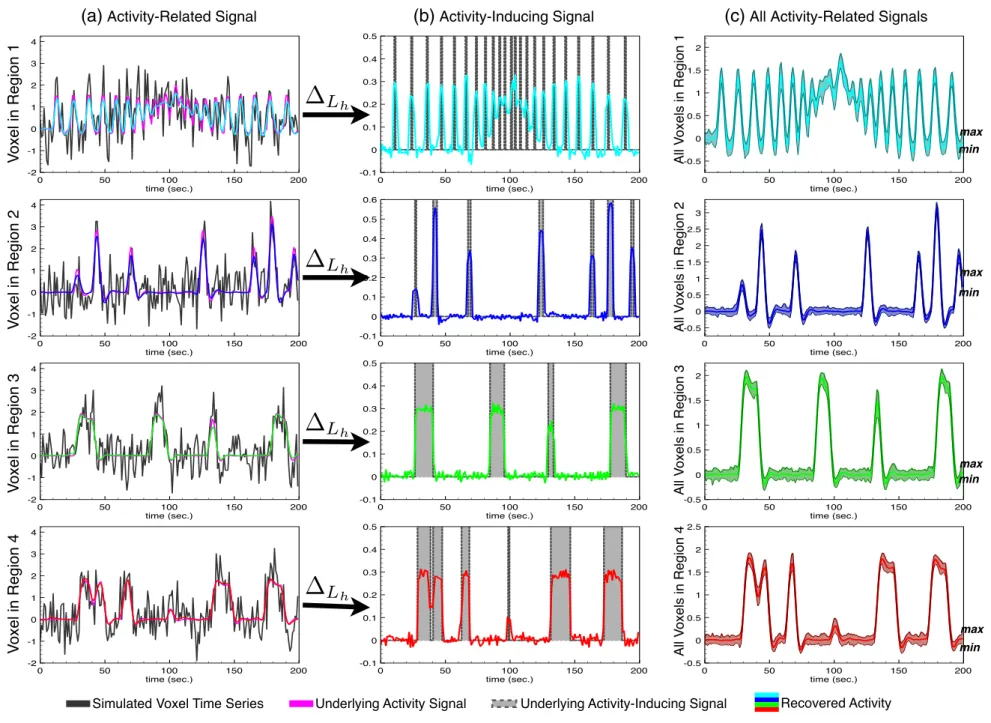
In order to validate the TA approach, we used a software phantom with 10× 10× 10 voxels divided into four regions. The activity-inducing signal was_ﬁxed within a region, but different between re-gions. Two regions had spike-like activity-inducing signals: region 1

has spike trains with gradually increasing inter stimulus interval (ISI) from 1 to 12 s, region 2 has short events with duration uniformly dis-tributed between [1,2]s. The other two regions have longer block-like activity (duration uniformly distributed between [1,…,15] s). The onset timings of the events have uniform distribution such that 12 and 6 events on average are generated in regions with spikes and blocks, respectively. A very short event is introduced into region 4 to test TA's robustness for short events in the middle of sustained events. All activity-inducing signals were sampled on a grid with temporal res-olution (TR) of 1 s and had 200 timepoints. The activity-induced signals were then convolved with the HRF and corrupted with i.i.d. Gaussian noise such that the signal-to-noise ratio (SNR) was 1 dB. We deﬁne the SNR as the ratio of signal power to noise power in logarithmic scale as SNR¼10 log10 ‖ x‖2 ‖y−x‖2 ! :

Fig. 3depicts the phantom and the associated time courses for

each region.

In this example, temporal and spatial regularization operate in ideal settings. First, the temporal differential operator is perfectly matched with the HRF (see Supplementary for the parametrization of the operator ΔLh). Second, the spatial regularization uses the same regions as the generative model.

Experimental data

We further evaluated TA with experimental data acquired on 3 sub-jects during a sparse event-related paradigm where resting state periods

Fig. 2.Flowchart of TA. Successive regularization in temporal and spatial domains is applied to the noisy BOLD time courses. Temporal regularization (blue window) inverts the

hemodynamic system by adopting a differential operator mimicking the inverse HRF and spatial regularization (red window) imposes smooth activations within the regions of an anatomical atlas. Finally, we obtain the activity-related signals and activity-inducing signals which reveal the neuronal-related activity.

(5)

were disrupted by 10 visual stimuli of 8 Hzﬂickering checkerboard of duration 1 s with onsets randomly chosen following a uniform distribution during the duration of the run. When no visual stimuli were presented, subjects were instructed to maintain visualﬁxation on a cross in the center of the screen. The experiment was conducted in a Siemens TIM Trio 3 T MR scanner with a 32-channel head coil. The fMRI data comprisedN= 160 (subjects 1 and 3) andN= 190 (subject 2)T2∗-weighted gradient echo-planar volumes (TR/TE/FA: 2 s/30 ms/85°, voxel size: 3.25 × 3.25 × 3.5 mm3_{, matrix = 64 × 64).} A T1-weighted MPRAGE anatomical image was also acquired during the MR session (192 slices, TR/TE/FA: 1.9 s/2.32 ms/9°, voxel size: 0.45×0.45×0.9 mm3_{, matrix=512×512).}

The preprocessing steps included realignment of the datasets to the

first scan of each subject and then spatial smoothing with a Gaussian smoother (FWHM= 5 mm). The spatial smoothing is not an essential step since TA also includes spatial regularization. However, the tempo-ral regularization parameter is tuned for each voxel with respect to the (estimated) noise level. Therefore, spatial smoothing provides a spatial-ly smoother estimate (less variations) of the noise level. Both steps were performed in the functional space of the subjects using SPM8 (FIL, UCL, UK). The anatomical AAL atlas (90 regions without the cere-bellum) was mapped onto each subject's functional space using the IBASPM toolbox (Alemán-Gómez et al., 2006; Tzourio-Mazoyer et al., 2002). The voxels' time courses labeled within the atlas were detrended using afirst-degree polynomial (i.e., linear trend) and slow oscillations (i.e., DCT basis function up to cut-off frequency of 1/250 Hz), and_finally scaled to have unit variance. As before, the temporal differential operator was chosen from linear inverse of the Balloon model (Khalidov et al., 2011) (see supplementary

section). The regularization parameters need to provide a compro-mise between data fitness and regularization cost. We calibrated the temporal regularization parameter such that the residual noise level converged to the pre-estimated noise level of the data fit, where pre-estimated noise level is derived from the median absolute deviation offine-scale wavelet coefficients (Daubechies, order 3). Then, for each iterationn, we update the temporal regularization pa-rameterλ1ð Þin(Algorithm 2, step 10) similar toChambolle (2004):

λ1ð Þi nþ1 ¼ Nσ˜ð Þi 1 2‖yði;·Þ−xði;·Þ n_‖2 2 λ1ð Þi n :

Spatial regularization parameter was empirically selected to be 5, which seemed to compensate well between temporal and spatial priors. The overall computation time for one dataset was around 5 h using a Linux cluster with Matlab (version 7.9).

After applying TA, we obtain three spatiotemporal datasets per subject: (1) the innovation signalus(i,t); (2) the activity-inducing

sig-nalu(i,t); (3) the activity-related signalx(i,t). The innovation signal is the driver of the others, which can be derived through linear convolu-tions. To summarize the rich amount of information available in these datasets, we computed the average of the activity-inducing signals within each anatomical region, and then obtained the Spearman cor-relation matrix between the averaged time courses. Corcor-relations were Fisher z-transformed and fed into a Ward's hierarchical clustering al-gorithm implemented in Matlab (Mathworks, Natick, MA, version (7.9) function linkage.m) to reveal the network structure contained in the activity-inducing signals. We selected two different levels to cut the dendrogram in order to show the evolution of clusters with

Fig. 3.The software phantom contains 4 regions in a cube that consists out of 10 × 10 × 10 voxels. Theﬁrst region (cyan, 300 voxels) was simulated as spike train with gradually

increasing ISI from 1 s to 12 s and the second region (blue, 210 voxels) was simulated with random events with uniform duration in (Afshin-Pour et al., 2012; Aguirre et al., 1998) seconds. The third region (green, 245 voxels) and the fourth region (red, 245 voxels) were simulated with random events with uniform duration in (Afshin-Pour et al., 2012; Chang and Glover, 2010) seconds. A very short event is inserted into region 4 (around 100 s). The time resolution was chosen as TR = 1 s. The activity-inducing signals (in gray) were convolved with HRF to obtain the BOLD activity for each region. Each voxel time series was then corrupted with i.i.d. Gaussian noise such that voxel time series had SNR of 1 dB.

(6)

(a) Activity-Related Signal

(b) Activity-Inducing Signal

(c) All Activity-Related Signals

Fig. 4.Results for the software phantom. The left column (a) shows simulated noisy data (black), underlying BOLD signals (magenta), and recovered activity-related signals of a random voxel in each region (cyan, blue, red, green, respec-tively). The middle column (b) shows the underlying activity-inducing signal (gray) and the associated recovered activity signals. Finally, the right column (c) shows all recovered activity-related signals from the software phantom indicated by their mean, maximum, minimum per region. Small deviations within each region are observed.

126 F.I. Karahano ğ lu et al. / NeuroImage 73 (2013) 121 – 134

(7)

respect to the inconsistency criterion that measures the deviation in each cluster.

Results

Synthetic data

InFigs. 4(a) and (b), we show, for randomly selected voxels in the

four different regions, the activity-related and activity-induced signals, respectively. The recovered activity-inducing signals match very closely with the ground-truth underlying activity with no prior information on the timing or duration of the simulated events. InFig. 4(ﬁrst row), we observe for region 1 that TA can resolve for events with ISI down to 2 TRs. The signal model is able to successfully recover different types of activity-inducing signals; i.e., short spike-like and long block-like stim-uli, especially the short event in region 4 is well detected, but with lower amplitude. InFig. 4(c), the variation of activity-related signals per region is summarized within the shaded area. Despite the relatively high level of noise in the simulated time courses, the recovered activity-inducing signals have small deviations across the voxels within each region. We refer the reader to Supplementary Figs. S.1 and S.2 to see the results without spatial regularization. Additional simulations were performed to a) simulate errors in the information provided by

the spatial template where TA demonstrated robustness against this model mismatch except that very brief activations may be undetected with large spatial discrepancies in Supplementary Fig. S.3, and b) variate the hemodynamic model used to generate the synthetic data (canonical HRF) with respect to the model used for the deconvolution (i.e. balloon model) which resulted in an expected time shift of the deconvolved sig-nals due to the differences in the temporal characteristics of both models, but without altering a successful recovery of the underlying ac-tivations in Supplementary Fig. S.4.

Experimental data

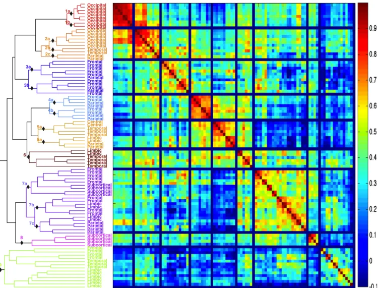
After applying TA, we averaged the region-averaged correlation ma-trix of the three subjects and obtained the dendrogram inFig. 5as a result of hierarchical clustering. We extracted functionally distinct clusters at coarse (high) and detailed (low) levels. In other words, going down from the highest level in the dendrogram (whole brain) the consistency in the hierarchy is gradually incremented until aﬁrst group of clusters is deﬁned (high-level), further increasing the consistency splits the clus-ters into subclusclus-ters which are meaningful segregations (low-level). At the high-level hierarchy, the brain is segregated into 9 global clusters (represented in different colors in the dendrogram); at the low-level hierarchy, 17 local networks (subclusters pinned from (1a) to (9) in

Fig. 5.Correlation matrix and corresponding clusters for TA activity-inducing signal. The dendrogram that reﬂects the hierarchical organization is shown on the left. Each color is

described with the regions correspond to a different cluster in high level clusters (total 9 clusters) which is evaluated via inconsistency measure. Note that low level clusters (marked with black pins in the dendrogram from (1a) to 9) subdivide the clusters resulting 17 clusters. The anatomical descriptions in the clusters are detailed inTable 1.

(8)

the dendrogram) are revealed.Fig. 6illustrates the high-level networks on the anatomical atlas. The extended anatomical descriptions in each (sub)cluster are listed inTable 1. We detail these clusters according to the order of the dendrogram.

The visual network makes up thefirst and second clusters, which is expected due to the stimulation and its strong coherence in resting state. Cluster 1 contains primary visual areas such as calcarinefissure, lingual gyrus and cuneus. Cluster 2 includes higher level visual areas extending towards ventral and dorsal visual pathways, inferior tempo-ral gyrus and superior parietal lobule, which are subclusters 2b and 2c, respectively. In Fig. 7 (bottom right), the region-averaged activity-inducing signal in the visual network confirms that the timing of the visual stimuli (red bars) is well recovered without any prior knowledge. Cluster 3 reveals a fronto-parietal network extending bi-lateral middle frontal gyrus, inferior frontal gyrus and inferior parie-tal lobule, which mimics the dorsal attention network (Fox et al., 2006) and involves in attentional mechanisms, especially for“salient and unattended events”(Corbetta and Shulman, 2002). Subclusters 3a and 3b represent the right and left lateralized fronto-parietal re-gions similar to Beckmann et al. (2005) and Damoiseaux et al.

(2006), respectively.

Cluster 4 reveals sensory-motor areas including primary motor cor-tex, primary somatosensory cortex as subcluster 4a, and supplementary

motor areas as subcluster 4b. Cluster 5 maps the auditory network where speech and language processing occur, including the Heschl gyrus, superior temporal gyrus (Wernicke's area) and inferior frontal gyrus. Cluster 6 involves bilateral midcingulate cortex, middle temporal gyrus as well as the right superior temporal gyrus. Cluster 7 consists of superior and middle frontal gyrus, anterior–posterior cingulate cortex (PCC) representing the default mode network (DMN) including thala-mus (Luca et al., 2006). The hierarchical clustering suggests that cluster 7 is segregated into its anterior (7a, 7b) and posterior (7c) components, which are known to be part of saliency and executive control networks

(Fox et al., 2006; Seeley et al., 2007), respectively. Similar subdivisions

of the DMN have also been reported recently using real-time fMRI neurofeedback (Van De Ville et al., 2012). Subcortical regions, putamen and pallidum, are engaged in cluster 8 bilaterally. Cluster 9 involves bi-lateral limbic regions, parahippocampal gyrus, hippocampus and amyg-dala, as well as olfactory bulb, gyrus rectus and temporal poles. For the sake of comparison the results of the same correlation and hierarchical clustering analysis on the original detrended data, i.e. without process-ing with our TA method, are shown in Supplementary Figs. S.5, S.6 and Table S.1. We observe that visual, motor and auditory networks are also identi_ﬁed, however, they are given different preferences in dendrogram (auditory network is cluster 8 instead on 5, motor is 7 instead of 4). In addition, the most prominent right–left lateralized fronto-parietal

CLUSTER 3

CLUSTER 6

CLUSTER 8

CLUSTER 1

CLUSTER 2

CLUSTER 4

CLUSTER 7

CLUSTER 9

CLUSTER 5

Fig. 6.Brain maps for the 9 high-level hierarchy clusters viewed from sagittal left (top left), sagittal cross-section in the middle (top right), top view (bottom left) and bottom

view (bottom right). The regions are generated using anatomical atlas in MNI space corresponding to the anatomical descriptions inTable 1. We recover the activity-related networks; i.e., primary and late visual networks in clusters 1 and 2, respectively. Additionally, the fronto-parietal network (cluster 3), motor and somatosensory regions (clus-ter 4) and auditory network (clus(clus-ter 5) as well as the default mode network (clus(clus-ter 7), subcorticals (clus(clus-ter 8) and limbic system (clus(clus-ter 9) are observed. The clus(clus-ters are nicely organized bilaterally.

(9)

network and anterior–posterior segregation of the default mode net-work is lost in the hierarchy.

Having identiﬁed coherent networks through clustering of the activity-inducing signals, we can try to represent the dynamics for brain regions revealed by TA. Fig. 7 depicts the average activity-inducing signals rearranged according to the clusters. While the stimu-lus timings are well discovered mainly in the cstimu-lusters corresponding to visual areas, we observe spontaneous activity in the visual network which does not correspond to visual stimuli (e.g., subject 2, cluster 1, around 300 s).

Fig. 8shows the dynamic activity-inducing maps of subject 2. Two

time courses are picked randomly from cuneus and PCC in order to track the temporal evolution of the task-related and spontaneous events. The positive and negative activations in PCC lagging the stim-ulus reﬂect the alternating structure of functional reorganization in the brain.

Finally, since the temporal prior of TA favors block-like activity-inducing signals, we evaluate the average block-length per region as the 4th quartile of the activity duration, seeFig. 9. It can be seen that regions in the visual clusters have relatively shorter average ac-tivity than other regions.

Discussion

Methodological implications

We have proposed TA to deconvolve fMRI data based on hemody-namic and anatomical properties of the brain. The objective is formulat-ed as a minimization problem where the convex cost function contains sparsity-inducing regularization terms in both the temporal and spatial dimensions. The optimization is performed using a state-of-the-art gen-eralized forward–backward scheme. The variational cost function is for-mulated assuming uncorrelated noise structure, nevertheless, an autoregressive noise model can be easily integrated into the framework. The colored noise should be whitened based on the estimated covari-ance of the residuals, which then leads to a weighted‘2-norm for the data-term of the cost function.

While TA does not require any timing information, it is not completely model-free neither—the three main underlying assump-tions are: (1) the operator to invert the hemodynamic system; (2) the sparse innovation signal that leads to block-type activity; (3) the ana-tomical atlas for spatial regularization. In the following discussion, we

Table 1

The list of regions in the clusters. The clustering algorithm delineates 9 and 17 clusters in the high and low-level hierarchies (also presented in dendrogram inFig. 5). Theﬁrst two clusters correspond to the visual networks. Note that cluster 3 (fronto-parietal network) is subdivided into its right (3a) and left (3b) compartments in the higher hierarchy. Likewise, cluster 7 (default mode) is divided into its anterior (7a, 7b) and posterior (7c) components.

Cluster Lobe Anatomical description 1a Occipital Calcarine Fissure Left

Occipital Calcarine Fissure Right Occipital Lingual Gyrus Left Occipital Lingual Gyrus Right Occipital Cuneus Left Occipital Cuneus Right

1b Occipital Superior Occipital Gyrus Left Occipital Superior Occipital Gyrus Right 2a Occipital Middle Occipital Gyrus Left

Occipital Inferior Occipital Gyrus Left Occipital Middle Occipital Gyrus Right Occipital Fusiform Gyrus Left Occipital Fusiform Gyrus Right Occipital Inferior Occipital Gyrus Right 2b Temporal Inferior Temporal Gyrus Left

Temporal Inferior Temporal Gyrus Right 2c Parietal Superior Parietal Gyrus Left

Parietal Superior Parietal Gyrus Right 3a Frontal Superior Frontal Gyrus (Orbital) Right

Frontal Inferior Frontal Gyrus (Orbital) Right Frontal Middle Frontal Gyrus (Orbital) Right Frontal Inferior Frontal Gyrus (Opercular) Right Frontal Inferior Frontal Gyrus (Triangular) Right Parietal Inferior Parietal Gyrus Right

3b Frontal Middle Frontal Gyrus (Orbital) Left Frontal Inferior Frontal Gyrus (Opercular) Left Frontal Inferior Frontal Gyrus (Triangular) Left Parietal Inferior Parietal Gyrus Left

Frontal Inferior Frontal Gyrus (Orbital) Left 4a Frontal Precentral Gyrus Left

Frontal Precentral Gyrus Right Parietal Postcentral Gyrus Left Parietal Postcentral Gyrus Right 4b Frontal Supplementary Motor Area Left

Frontal Supplementary Motor Area Right Parietal Paracentral Lobule Left Parietal Paracentral Lobule Right 5a Central Rolandic Operculum Left Central Rolandic Operculum Right Temporal Superior Temporal Gyrus Left Temporal Heschl Gyrus Right Temporal Heschl Gyrus Left 5b Limbic Insula Left

Limbic Insula Right

Parietal SupraMarginal Gyrus Left Parietal SupraMarginal Gyrus Right 6 Limbic Medial Cingulate Cortex Left

Limbic Medial Cingulate Cortex Right Temporal Superior Temporal Gyrus Right Temporal Middle Temporal Gyrus Left Temporal Middle Temporal Gyrus Right Temporal Temporal Pole (Superior) Right 7a Frontal Superior Frontal Gyrus (Orbital) Left

Frontal Middle Frontal Gyrus Left

Frontal Superior Frontal Gyrus (Dorsolateral) Left Frontal Superior Frontal Gyrus (Dorsolateral) Right Frontal Middle Frontal Gyrus Right

Subcortical Caudate Nucleus Left Subcortical Caudate Nucleus Right Subcortical Thalamus Left Subcortical Thalamus Right

7b Frontal Superior Frontal Gyrus (Medial) Left Frontal Superior Frontal Gyrus (Medial) Right Limbic Anterior Cingulate Cortex Left Limbic Anterior Cingulate Cortex Right

Frontal Superior Frontal Gyrus (Medial–Orbital) Left Frontal Superior Frontal Gyrus (Medial–Orbital) Right 7c Limbic Posterior Cingulate Cortex Left

Limbic Posterior Cingulate Cortex Right Parietal Precuneus Left

(continued on next page)

Table 1(continued)

Cluster Lobe Anatomical description Parietal Precuneus Right Parietal Angular Gyrus Left Parietal Angular Gyrus Right 8 Subcortical Putamen Left

Subcortical Pallidum Left Subcortical Putamen Right Subcortical Pallidum Right 9 Frontal Olfactory Cortex Left

Frontal Olfactory Cortex Right Frontal Gyrus Rectus Left Frontal Gyrus Rectus Right Temporal Temporal Pole (Superior) Left Temporal Temporal Pole (Middle) Left Temporal Temporal Pole (Middle) Right Limbic Hippocampus Left

Limbic ParaHippocampal Gyrus Left Limbic Hippocampus Right Limbic ParaHippocampal Gyrus Right Limbic Amygdala Left

(10)

ﬁrst highlight each of these assumptions and then the related work in theﬁeld.

Hemodynamics

We use the ﬁrst-order Volterra kernel of the non-linear balloon model to characterize the differential operator that relates activity-inducing signal with fMRI BOLD. It is well known that this model is lim-ited since high variability of HRF within and across subjects has been ob-served (Handwerker et al., 2004). Additionally, the HRF might be different for task-related versus spontaneous activity. Nevertheless, the current approach seems to be a reasonable starting point. It can be re-placed by other more sophisticated models, such as the one bySotero

and Trujillo-Barreto (2007), which accounts for the difference in

excit-atory and inhibitory neuronal activity. Another possible extension is to

ﬁne-tune the HRF operator (e.g., per region or even voxel) by alternating between the optimization of the activity-inducing signal and the HRF pa-rameters (4 zeros and 1 pole) to obtain the region/voxel speciﬁc HRF similar to parcel based HRF estimation methods inChaari et al. (2013)

andVincent et al. (2010).

Sparse innovation signal

The core principle of TA consists of deﬁning an innovation signal that should be sparse if the experimentally-evoked or spontaneous brain ac-tivity has an underlying acac-tivity-inducing signal that is block-type. We have demonstrated that this is a strong prior, which allows us to recover paradigm-related activity without any timing information, yet also

without constraints on the block length of the activity-inducing signal. Besides, this signal model goes beyond the traditional Fourier view-point; i.e., for signals with the same regularization cost, the Fourier spectrum can vary from“simple”(e.g., periodic timing) to“complex” depending on the relative timing of the events.

Here we have imposed the‘1-norm for the temporal prior, which is the most common sparsity-pursuing norm. Although the Bayesian interpretation of the variational framework is beyond the scope of this paper, we would like to mention that stochastic processes gener-ating sparse (innovation) signals are an active research in signal pro-cessing and applied statistics. In particular, the continuous-domain deﬁnition of this type of “noise” requires proper analytical tools

(Unser et al., 2011). An intriguing research avenue for generative

models of activity-inducing signals, is the choice of the stochastic pro-cess to generate the innovation signal.

Anatomical atlas

Many methods for fMRI data analysis rely upon Gaussian smoothing to improve the SNR. The spatial regularization of TA adds a structured-sparsity constraint by favoring smoothing within anatomical regions, but sparsity across. This is obtained by a mixed norm expressed on the Laplacian of the volume. For our settings of the spatial regularization parameter, we obtain more consistent activity-inducing signals within the regions, but at the same time the signals are not necessarily the same (e.g., seeFig. 8).

ACTIVITY-INDUCING SIGNAL SUBJECT 1 ACTIVITY-INDUCING SIGNAL SUBJECT 2

AVERAGE ACTIVITY IN CLUSTER 1 (OCCIPITAL) ACTIVITY-INDUCING SIGNAL SUBJECT 3

PARADIGM CLUSTER 1 CLUSTER 2 CLUSTER 3 CLUSTER 4 CLUSTER 5 CLUSTER 6 CLUSTER 7 CLUSTER 8 CLUSTER 9 PARADIGM CLUSTER 1 CLUSTER 2 CLUSTER 3 CLUSTER 4 CLUSTER 5 CLUSTER 6 CLUSTER 7 CLUSTER 8 CLUSTER 9 PARADIGM CLUSTER 1 CLUSTER 2 CLUSTER 3 CLUSTER 4 CLUSTER 5 CLUSTER 6 CLUSTER 7 CLUSTER 8 CLUSTER 9

Fig. 7.Activity-inducing signals per region and subject. Clearly, the activity-inducing signal in the visual regions (clusters 1 and 2) follows the visual paradigm closely. Moreover, we

observe the intrinsic brain activity, for example, a spontaneous event (in black contour) occurs around 300 s in subject 2 which is followed by negative activation in clusters 4–7 (posterior default mode network). The average activity in the occipital lobe (bottom right) matches with the visual stimulation.

(11)

1 -1 1 -1 1 -1

Positive

Activation in

PCC

following the

stimulus

1

-1

Negative

Activation in

PCC

following the

stimulus

Activation before stimulus

Activation after stimulus

t

Fig. 8.Reconstructed dynamic activity-inducing maps for subject 2 (see supplementary for the movie). Time courses from cuneus and PCC are plotted in white and yellow, respectively. The stimulus time course is shown in magenta. In the

ﬁrst frame, the activity maps are illustrated for two instances (top row around 90 s and bottom row around 250 s). The left and right columns show the activation maps before and after the stimulus, respectively. PCC lags the stimuli with positive (top row) or negative response (bottom row).

131 F.I. Karahano ğ lu et al. / NeuroImage 73 (2013) 121 – 134

(12)

The anatomical atlas is still a limitation of TA since it is not specific to the subject. An interesting option would be to make the atlas data-adaptive. For example, the regions could be re-estimated after a couple of iterations of the algorithm (Bellec et al., 2010) or joint estima-tion of HRF and HRF-defined region identification could be adapted into

TA (Chaari et al., 2012). Another option would be to apply TA to the time

courses recovered from a mode-decomposition (e.g., ICA).

Related methods

We mention in more detail three other deconvolution methods that have deployed similar ideas to recover activity-inducing signals

(Gaudes et al., 2011, 2013; Hernandez-Garcia and Ulfarsson, 2011;

Khalidov et al., 2011). All these methods operate solely in the

tempo-ral domain, and do not add spatial information into their framework. Also, the temporal prior of these methods is a“synthesis prior”, which means that an explicit dictionary of atoms is built. In

Khalidov et al. (2011), wavelets (“activelets”) tailored to the

hemo-dynamic system are designed and used to decompose BOLD fMRI sig-nals that should ideally lead to sparse activelet coefﬁcients if the activity is spike-like. In Gaudes et al. (2011) and Gaudes et al.

(2013), a dictionary with all possible shifts of the canonical HRF is

constructed to recover spike-like activity. InHernandez-Garcia and

Ulfarsson (2011), the dictionary combines spike-like and block-like

atoms with two different regularization terms, which raises the issue how to choose the regularization parameters to adapt to the ratio of spikes and blocks for each voxel. Alternatively, the temporal regularization of TA uses an“analysis prior”, which is much more

ﬂexible (e.g., blocks of different lengths do not need to be speciﬁed explicitly, which would be prohibitive).

Dynamics of activity-inducing maps

When visualizing the activity-inducing signals obtained by TA on dy-namic brain maps, we can easily recognize the presence and onsets of the visual stimuli. However, the data is much richer and many spontaneous events are captured as well; e.g., strong activity in the visual network of subject 2 during theﬁnal resting period (Fig. 7). Interestingly, activity-inducing signals reveal some non-stationary relationships between the different brain regions; e.g., as can be seen fromFig. 8, the signals from PCC and visual cortex are sometimes negatively correlated, and some-times positively. This non-stationary behavior is also suggested in a time-frequency coherence analysis of fMRI (Chang and Glover, 2010).

Moreover, a recent work bySmith et al. (2012)exploits temporal and spatial ICA on high resolution data to reveal the temporally-independent and spatially overlapping activity maps called“ tempo-ral functional modes”. The authors show that different networks share common subcomponents of each other, that is, one brain region does not necessarily belong to a distinct functional network.

Hierarchical clustering

As a post-processing step, clustering the activity-inducing signals obtained by TA allows us to get a better understanding of the data. We obtain functionally plausible networks (many bilateral) reflecting both task-related and spontaneous activity. It is somewhat intriguing that activity of both task-related and resting-state networks is so well captured. While it is known that spontaneous activity continues dur-ing task and configurations similar to resting-state networks are formed (Fox and Raichle, 2007), it also means that our model for block-like activity-inducing signals is well suited for both types of ac-tivity. This raises the interesting hypothesis for future studies wheth-er resting-state activity is rathwheth-er block-like (with long durations on average) versus sinusoidalfluctuations (with low frequency).

The block model for the activity-inducing signal is also veryﬂexible as it does not impose any duration. From the duration map, we clearly observe that the regions in the visual cortex have shorter duration whereas fronto-parietal regions have relatively the longest duration.

The quality of the clustering (i.e., high correlation within and low cor-relation between clusters) is higher for the results obtained on TA-regularized activity-inducing signals; seeFigs. 5 and 6and compare with Supplementary Figs. S.5 and S.6. For non-TA processed signals, we obtain higher variation in the large clusters (especially clusters 3 and 4). Visual, motor and auditory networks match most with the results of TA, however, their rank in dendrogram is different (auditory network is clus-ter 8 instead on 5, motor is 7 instead of 4). Moreover, the most prominent right–left lateralized fronto-parietal network and anterior–posterior seg-regation of the default mode networks is lost in the hierarchy.

Conclusion

We have introduced TA, a new analysis tool that essentially aims at revealing the activity-inducing driver of BOLD fMRI. Using syn-thetic and experimental data, we evaluated TA's ability to recover the underlying activity without timing information of cognitive

Fig. 9.Average block length for the region-averaged activity-inducing signals. Regions in the visual network have relatively shorter average activity than other regions.

(13)

tasks or stimuli, as well as the intrinsic brain activity. The method is formulated within the variational framework and solved using a con-vex optimization scheme where temporal and spatial priors are han-dled iteratively. This study allows for exploring brain dynamics while retaining both hemodynamics and spatial coherence in the brain and hence constitute a good candidate to reveal the both task-related and spontaneous activity. The application of TA to un-cover dynamic activity-inducing maps could also be a powerful tool prior to more advanced clustering techniques.

Acknowledgments

This work was supported in part by the Swiss National Science Foundation under grant PP00P2-123438 and in part by the Center for Biomedical Imaging (CIBM) of the Geneva-Lausanne Universities & Hospitals and the EPFL.

Appendix A. Algorithm

The generalized forward–backward splitting (Raguet et al., 2012) aims to minimize a convex cost function that consists of a quadratic dataﬁtting term and multiple regularization terms. The solution is obtained by incorporating the solutions of each convex regularization problem separately which are deﬁned as

˜ xT¼arg min_x 1 2‖y−x‖ 2 Fþ XV i¼1 λ1ð Þi‖ΔLfxði;·Þg‖1¼proxRTð Þy; ðA:1Þ ˜ xS¼arg min_x 1 2‖y−x‖F 2 þX N t¼1 λ2ð Þt‖Δfxð·;tÞg‖ð2;1Þ¼proxRSð Þy: ðA:2Þ The solutions of the above problems correspond to proximal maps to the temporal and spatial regularization terms in Eqs.(8) and (10)

(Combettes and Wajs, 2005). These variational formulations are

nonquadratic; i.e., direct solutions do not exist, and hence iterative al-gorithms should be employed. Forward–backward splitting method

(Combettes and Wajs, 2005) applies on functionals when the

regular-ization term is a non-smooth convex function and the data-term is a smooth differentiable function with aﬁnite Lipschitz constant. In the forward step, a gradient descent is applied for data-term and in the backward step, proximal map is computed for the regularization function. We exploit the dual deﬁnitions of ‘1-norm and ‘2-norm

(Baritaux et al., 2011; Chambolle, 2004) toﬁnd the solution of each

proximal map, and employ “fast gradient projection” (FGP) (Beck

and Teboulle, 2009) to achieve faster convergence. Here, we

formu-late the generalized algorithm (detailed inRaguet et al., 2012). Algorithm 1. Spatio-temporal regularization x˜¼arg minx12‖y−x‖

2 Fþ RTð Þþ Rx Sð Þx

Let's consider the temporal term where the cost function is

CTðxð Þi;⋅Þ ¼ Fð Þ þx XV

i¼1

λ1ð Þi‖ΔLfxð Þi;⋅g‖1; ðA:3Þ

where the smooth data-term isFð Þ ¼x 1 2‖y−x‖

2

F. The regularization term is‘1-norm; i.e., a non-smooth function. Let's call that the mini-mizer ofCTisx*, then ∂CT x ð Þ∈∇Fð Þ þx ∂RT x ð Þ ¼0; x−μ∇Fð Þx∈ðIþμ∂RTÞx ð Þ; x¼ðIþμ∂RTÞ− 1 x−μ∇Fð Þx ð Þ ¼prox_μ_R T x ₋_μ_∇_F_{ð Þ}_x ð Þ:

The iterative solution consists of solving for forward term, i.e., xforward¼xn₋_μ_∇_F_{ð Þ}_x _{and backward term, i.e.,} _xnþ1_¼_prox

μRT

xforward

. Speciﬁcally, forward solution in Eq.(A.3)is straightforward and minimizer depends only on the proximal map withxforward=y

andx¼prox_R_Tð Þ.y

There is no direct analytical solution for minimizing the primal problem in Eq.(A.3). Instead the dual formulation provides an easier interpretation. The dual-norm is deﬁned as

‖ΔLfxð Þi;⋅g‖1¼max ‖p‖b1hΔLfxð Þi;⋅g;pð Þi;⋅i: Then, min x CT¼minx _‖maxp‖≤1 1 2‖y−x‖ 2 Fþ XV i¼1 λ1ð Þi xð Þi;⋅;Δ T Lfpð Þi;⋅g D E ;

since function is convex inxconcave inpwe interchange min_–max and at the saddle point the primal and dual formulations lead to the same solution ¼max ‖p‖≤1minx 1 2‖y−x‖ 2 Fþ XV i¼1 λ1ð Þi xð Þi;⋅;Δ T Lfpð Þi;⋅g D E ;

whereΔLTcorresponds to the adjoint ofΔL, i.e.,ΔLT[t] =ΔL[−t].

This algorithm has a fast convergence due to steps 7 and 8 (Beck

and Teboulle, 2009; Combettes and Wajs, 2005; Raguet et al., 2012)

and a robust update of the regularization parameterλ(Chambolle, 2004). The algorithm for spatial regularization can be achieved simi-larly for each volumetexploiting the dual-norm of‘ð2;1Þ-norm into the formulation instead of‘1-norm (Baritaux et al., 2011). Discrete implementation of operatorΔLcan be efﬁciently done by constructing

stable (causal and anti-causal)ﬁlters. We refer toKarahanoglu et al.

(2011)for implementation details andﬁlter coefﬁcients.

Algorithm 2. Temporal regularization prox_R

Tð Þ ¼y arg minx 1 2‖y−x‖ 2 Fþ ∑V i¼1λ1ð Þi‖ΔLf gx ‖1

INPUTS:Noisy fmri datay,

1: Initialize:n←1; ^x0

T¼0; x^0S¼0;x˜

0_¼ 0;,

2:Repeat

3: Solve for temporal prior:x^nþ1

T ¼^xnTþproxRT x˜ n −^xn Tþy −x˜n 4: Solve for spatial prior:^xnþ1

S ¼^xnSþproxRS x˜ n −^xn Sþy −x˜n 5: Updatex˜nþ1¼^xnþ1 T =2þ^xnSþ1=2 6: n←n+ 1

7:untilconvergence or number of maximum iterations are reached.

INPUTS:Noisy fmri datay, Differential operatorΔL, Noise estimateσ˜that is, median

absolute deviation of the second order wavelet coefﬁcients ofyand spectral normc c>sup ω Δ^L e jω 2¼sup ω ∏4 m¼1j1−eαme−jω_j₂ j1−eγ1e−jωj2_: 1:foreach voxeli= 1 toVdo

2: n←1 3: Initialize:k1 = 1, p0 = 0,x(i,⋅)1 = 0,v1 = 0 andλ1ð Þi1¼σ˜ð Þi 4: repeat 5: Updatepn =ΔL{y(i,⋅)}/(λ1(i)nc) + (I−ΔLΔLT/c){vn} 6: Update pn = clip(pn

) where clip(⋅) denotes the element-wise clipping function,

clip(⋅) = sign(⋅)min(|⋅|, 1), 7: Updateknþ1¼1þ ffiffiffiffiffiffiffiffiffiffiffiffiffiffiffiffi 1þ4_{ð Þ}kn2 q 2 8: Updatevnþ1_¼_pn_þkn₋1 knþ1 pn−pn−1 9: Setxð Þi;⋅n_¼ yð Þi;⋅−λ1ð ÞinΔTLf gp; 10: Updateλ1ð Þinþ1¼1_2‖yð Þ−i;⋅Nσ˜xð Þið Þi;⋅n_‖2 2λ1 i ð Þn_, 11: n←n+ 1

12: untilconvergence or number of maximum iterations are reached.

(14)

Appendix B. Supplementary data

Supplementary data to this article can be found online athttp://

dx.doi.org/10.1016/j.neuroimage.2013.01.067.

References

Afshin-Pour, B., Hossein-Zadeh, G.A., Strother, S.C., Soltanian-Zadeh, H., 2012. Enhanc-ing reproducibility of fMRI statistical maps usEnhanc-ing generalized canonical correlation analysis in NPAIRS framework. Neuroimage 60, 1970–1981.

Aguirre, G., Zarahn, E., D'Esposito, M., 1998. The variability of human, BOLD hemody-namic responses. Neuroimage 8, 360–369.

Alemán-Gómez, Y., Melie-Garćia, L., Valdés-Hernandez, P., 2006. IBASPM: toolbox for automatic parcellation of brain structures. 12th Annual Meeting of the Organiza-tion for Human Brain Mapping, 27.

Baritaux, J.C., Hassler, K., Bucher, M., Sanyal, S., Unser, M., 2011. Sparsity-driven recon-struction for FDOT with anatomical priors. IEEE Trans. Med. Imaging 30, 1143–1153.

Baumgartner, R., Ryner, L., Richter, W., Summers, R., Jarmasz, M., Somorjai, R., 2000. Comparison of two exploratory data analysis methods for fMRI: fuzzy clustering vs. principal component analysis. Magn. Reson. Imaging 18, 89–94.

Beck, A., Teboulle, M., 2009. Fast gradient-based algorithms for constrained total variation image denoising and deblurring problems. IEEE Trans. Image Process. 18, 2419–2434. Beckmann, C.F., Smith, S.M., 2004. Probabilistic independent component analysis for

fMRI. IEEE Trans. Med. Imaging 23, 137–152.

Beckmann, C.F., DeLuca, M., Devlin, J.T., Smith, S.M., 2005. Investigations into resting-state connectivity using independent component analysis. Philos. Trans. R. Soc. Lond. B Biol. Sci. 360, 1001–1013.

Bellec, P., Rosa-Neto, P., Lyttelton, O.C., Benali, H., Evans, A.C., 2010. Multi-level boot-strap analysis of stable clusters in resting-state fMRI. Neuroimage 51, 1126–1139. Biswal, B., Yetkin, F.Z., Haughton, V., Hyde, J., 1995. Functional connectivity in the motor cortex of resting human brain using echo-planar MRI. Magn. Reson. Med. 34, 537–541. Calhoun, V., Adali, T., 2006. Unmixing fMRI with independent component analysis. IEEE

Eng. Med. Biol. Mag. 25, 79–90.

Chaari, L., Forbes, F., Vincent, T., Ciuciu, P., 2012. Adaptive hemodynamic-informed parcellation of fMRI data in a variational joint detection estimation framework. 15th Proc. MICCAI, LNCS. Springer Verlag, pp. 180–188.

Chaari, L., Vincent, T., Forbes, F., Dojat, M., Ciuciu, P., 2013. Fast joint detection-estima-tion of evoked brain activity in event-related fMRI using a variadetection-estima-tional approach. IEEE Trans. Med. Imaging.http://dx.doi.org/10.1109/TMI.2012.2225636. Chambolle, A., 2004. An algorithm for total variation minimization and applications.

J. Math. Imaging Vision 20, 89–97.

Chang, C., Glover, G.H., 2010. Time-frequency dynamics of resting-state brain connec-tivity measured with fMRI. Neuroimage 50, 81–98.

Cole, D.M., Smith, S.M., Beckmann, C.F., 2010. Advances and pitfalls in the analysis and interpretation of resting-state fMRI data. Front. Syst. Neurosci. 4.

Combettes, P., Wajs, V., 2005. Signal recovery by proximal forward–backward splitting. Multiscale Model. Simul. 4, 1168–1200.

Corbetta, M., Shulman, G.L., 2002. Control of goal-directed and stimulus-driven atten-tion in the brain. Nat. Rev. Neurosci. 3, 201–215.

Damoiseaux, J.S., Rombouts, S.A.R.B., Barkhof, F., Scheltens, P., Stam, C.J., Smith, S.M., Beckmann, C.F., 2006. Consistent resting-state networks across healthy subjects. Proc. Natl. Acad. Sci. 103, 13848–13853.

Evans, J., Todd, R., Taylor, M., Strother, S., 2010. Group speciﬁc optimisation of fMRI processing steps for child and adult data. Neuroimage 50, 479–490.

Flandin, G., Penny, W.D., 2007. Bayesian fMRI data analysis with sparse spatial basis function priors. Neuroimage 34, 1108–1125.

Fox, M.D., Raichle, M.E., 2007. Spontaneousﬂuctuations in brain activity observed with fMRI. Nat. Rev. Neurosci. 8, 700–711.

Fox, M.D., Corbetta, M., Snyder, A.Z., Vincent, J.L., Raichle, M.E., 2006. Spontaneous neu-ronal activity distinguishes human dorsal and ventral attention systems. Proc. Natl. Acad. Sci. 103, 10046–10051.

Friston, K.J., Fletchera, P., Josephs, O., Holmes, A., Rugg, M.D., Turner, R., 1998. Event-related fMRI: characterizing differential responses. Neuroimage 7, 30–40.

Friston, K.J., Mechelli, A., Turner, R., Price, C.J., 2000. Nonlinear responses in fMRI: the bal-loon model, Volterra kernels, and other hemodynamics. Neuroimage 12, 466–477. Friston, K., Trujillo-Barreto, N., Daunizeau, J., 2008. DEM: a variational treatment of

dy-namic systems. Neuroimage 41, 849–885.

Friston, K.J., Stephan, K., Daunizeau, J., 2010. Generalisedﬁltering. Math. Probl. Eng. 2010.http://dx.doi.org/10.1155/2010/621670.

Gaudes, C.C., Petridou, N., Dryden, I.L., Bai, L., Francis, S.T., Gowland, P.A., 2011. Detec-tion and characterizaDetec-tion of single-trial fMRI BOLD responses: paradigm free map-ping. Hum. Brain Mapp. 32, 1400–1418.

Gaudes, C.C., Petridou, N., Francis, S.T., Dryden, I.L., Gowland, P.A., 2013. Paradigm free mapping with sparse regression automatically detects single-trial fMRI BOLD re-sponses. Hum. Brain Mapp. 39, 501–518.

Gitelman, D., Penny, W., Ashburner, J., Friston, K., 2003. Modeling regional and psycho-physiologic interactions in fMRI: the importance of hemodynamic deconvolution. Neuroimage 19, 200–207.

Glover, G.H., 1999. Deconvolution of impulse response in event-related BOLD fMRI. Neuroimage 9, 416–429.

Gusnard, D.A., Raichle, M.E., 2001. Searching for a baseline: functional imaging and the resting human brain. Nat. Rev. Neurosci. 2, 685–694.

Handwerker, D.A., Ollinger, J.M., D'Esposito, M., 2004. Variation of BOLD hemodynamic responses across subjects and brain regions and their effects on statistical analyses. Neuroimage 21, 1639–1651.

Harrison, L., Penny, W., Flandin, G., Ruff, C., Weiskopf, N., Friston, K., 2008. Graph-partitioned spatial priors for functional magnetic resonance images. Neuroimage 43, 694–707.

Havlicek, M., Friston, K.J., Jan, J., Brazdil, M., Calhoun, V.D., 2011. Dynamic modeling of neuronal responses in fMRI using cubature Kalmanﬁltering. Neuroimage 56, 2109–2128.

Hernandez-Garcia, L., Ulfarsson, M.O., 2011. Neuronal event detection in fMRI time se-ries using iterative deconvolution techniques. Magn. Reson. Imaging 29, 353–364. Karahanoglu, F.I., Bayram, I., Van De Ville, D., 2011. A signal processing approach to

generalized 1-D total variation. IEEE Trans. Signal Process. 59, 5265–5274. Khalidov, I., Van De Ville, D., Fadili, J., Unser, M., 2007. Activelets and sparsity: a new

way to detect brain activation from fMRI data. Proceedings of the SPIE Conference on Mathematical Imaging: Wavelet XII, San Diego CA, USA, pp. 1–8.

Khalidov, I., Fadili, J., Lazeyras, F., Van De Ville, D., Unser, M., 2011. Activelets: Wavelets for sparse representation of hemodynamic responses. Signal Process. 91, 2810–2821. Kirsch, A., 1996. An introduction to the mathematical theory of inverse problems, 2nd

edition. Applied Mathematical Sciences, vol. 120. Springer.

Liu, Y., Gao, J.H., Liu, H.L., Fox, P.T., 2000. The temporal response of the brain after eating revealed by fMRI. Nature 405, 1058–1062.

Lopes, R., Lina, J., Fahoum, F., Gotman, J., 2012. Detection of epileptic activity in fmri without recording the EEG. Neuroimage 60, 1867–1879.

Luca, M.D., Beckmann, C., Stefano, N.D., Matthews, P., Smith, S., 2006. fMRI resting state networks deﬁne distinct modes of long-distance interactions in the human brain. Neuroimage 29, 1359–1367.

Lund, T.E., Madsen, K.H., Sidaros, K., Luo, W.L., Nichols, T.E., 2006. Non-white noise in fMRI: does modelling have an impact? Neuroimage 29, 54–66.

Makni, S., Idier, J., Vincent, T., Thirion, B., Dehaene-Lambertz, G., Ciuciu, P., 2008. A fully Bayesian approach to the parcel-based detection-estimation of brain activity in fMRI. Neuroimage 41, 941–969.

Morgan, V.L., Li, Y., Abou-Khalil, B., Gore, J.C., 2008. Development of 2dTCA for the de-tection of irregular, transient BOLD activity. Hum. Brain Mapp. 29, 57–69. Petridou, N., Gaudes, C.C., Dryden, I.L., Francis, S.T., Gowland, P., 2012. Periods of rest in

fMRI contain individual spontaneous events which are related to slowlyﬂ uctuat-ing spontaneous activity. Hum. Brain Mapp.http://dx.doi.org/10.1002/hbm.21513. Raguet, H., Fadili, J., PeyrŽ, G., 2012. Generalized forward–backward splitting.http://

arxiv.org/abs/1108.4404v3.

Raichle, M.E., 2006. The brain's dark energy. Science 314, 1249–1250.

Riera, J.J., Watanabe, J., Kazuki, I., Naoki, M., Aubert, E., Ozaki, T., Kawashima, R., 2004. A state-space model of the hemodynamic approach: nonlinearﬁltering of BOLD sig-nals. Neuroimage 21, 547–567.

Rudin, L.I., Osher, S., Fatemi, E., 1992. Nonlinear total variation based noise removal al-gorithms. Proceedings of the Eleventh Annual International Conference of the Cen-ter for Nonlinear Studies on Experimental mathematics: Computational Issues in Nonlinear Science. Elsevier North-Holland, Inc., pp. 259–268.

Seeley, W.W., Menon, V., Schatzberg, A.F., Keller, J., Glover, G.H., Kenna, H., Reiss, A.L., Greicius, M.D., 2007. Dissociable intrinsic connectivity networks for salience pro-cessing and executive control. J. Neurosci. 27, 2349–2356.

Smith, M., Fahrmeir, L., 2007. Spatial Bayesian variable selection with application to functional magnetic resonance imaging. J. Am. Stat. Assoc. 102, 417–431. Smith, S.M., Miller, K.L., Moeller, S., Xu, J., Auerbach, E.J., Woolrich, M.W., Beckmann,

C.F., Jenkinson, M., Andersson, J., Glasser, M.F., Essen, D.C.V., Feinberg, D.A., Yacoub, E.S., Ugurbil, K., 2012. Temporally-independent functional modes of spon-taneous brain activity. Proc. Natl. Acad. Sci. 8, 3131–3136.

Sotero, R.C., Trujillo-Barreto, N.J., 2007. Modelling the role of excitatory and inhibitory neuronal activity in the generation of the BOLD signal. Neuroimage 35, 149–165. Thirion, B., Flandin, G., Pinel, P., Roche, A., Ciuciu, P., Poline, J.B., 2006. Dealing with the

shortcomings of spatial normalization: multi-subject parcellation of fMRI datasets. Hum. Brain Mapp. 27, 678–693.

Tzourio-Mazoyer, N., Landeau, B., Papathanassiou, D., Crivello, F., Etard, O., Delcroix, N., Mazoyer, B., Loliot, M., 2002. Automated anatomical labeling of activations in SPM using a macroscopic anatomical parcellation of the MNI MRI single-subject brain. Neuroimage 15, 273–289.

Unser, M., Tafti, P.D., Sun, Q., 2011. A uniﬁed formulation of Gaussian vs. sparse sto-chastic processes part I: continuous-domain theory.http://arxiv.org/abs/1108. 6150v1.

Van De Ville, D., Jhooti, P., Haas, T., Kopel, R., Lovblad, K.O., Schefﬂer, K., Haller, S., 2012. Re-covery and spatio-temporal segregation of default mode subnetworks. Neuroimage 63, 1175–1781.

Vincent, T., Risser, L., Ciuciu, P., 2010. Spatially adaptive mixture modeling for analysis of fMRI time series. IEEE Trans. Med. Imaging 29, 1059–1074.

Yuan, M., Lin, Y., 2006. Model selection and estimation in regression with grouped vari-ables. J. R. Stat. Soc. 68, 49–67.

Zibulevsky, M., Elad, M., 2010. L1–L2 optimization in signal and image processing. IEEE Signal Proc. Mag. 27, 76–88.