Memorial Sloan-Kettering Cancer Center
Memorial Sloan-Kettering Cancer Center, Dept. of Epidemiology
& Biostatistics Working Paper Series
Year Paper
Sparse Integrative Clustering of Multiple
Omics Data Sets
Ronglai Shen
∗Sijian Wang
†Qianxing Mo
‡∗Memorial Sloan-Kettering Cancer Center, shenr@mskcc.org
†University of Wisconsin, Madison
‡Baylor College of Medicine
This working paper is hosted by The Berkeley Electronic Press (bepress) and may not be commer-cially reproduced without the permission of the copyright holder.
http://biostats.bepress.com/mskccbiostat/paper24
Sparse Integrative Clustering of Multiple
Omics Data Sets
Ronglai Shen, Sijian Wang, and Qianxing Mo
Abstract
High resolution microarrays and second-generation sequencing platforms are pow-erful tools to investigate genome-wide alterations in DNA copy number, methyla-tion, and gene expression associated with a disease. An integrated genomic profil-ing approach measurprofil-ing multiple omics data types simultaneously in the same set of biological samples would render an integrated data resolution that would not be available with any single data type. In a previous publication (Shen et al., 2009), we proposed a latent variable regression with a lasso constraint (Tibshirani, 1996) for joint modeling of multiple omics data types to identify common latent vari-ables that can be used to cluster patient samples into biologically and clinically relevant disease subtypes. The resulting sparse coefficient vectors (with many zero elements) can be used to reveal important genomic features that have signifi-cant contributions to the latent variables. In this study, we consider a combination of lasso, fused lasso (Tibshirani et al., 2005) and elastic net (Zou & Hastie, 2005) penalties and use an iterative ridge regression to compute the sparse coefficient vectors. In model selection, a uniform design (Fang & Wang, 1994) is used to seek “experimental” points that scattered uniformly across the search domain for efficient sampling of tuning parameter combinations. We compared our method to sparse singular value decomposition (SVD) and penalized Gaussian mixture model (GMM) using both real and simulated data sets. The proposed method is applied to integrate genomic, epigenomic, and transcriptomic data for subtype analysis in breast and lung cancer data sets.
Sparse Integrative Clustering of Multiple Omics Data
Sets
Ronglai Shen
∗Department of Epidemiology and Biostatistics,
Memorial Sloan-Kettering Cancer Center, New York, NY 10065, U.S.A.
Sijian Wang
Department of Biostatistics and Medical Informatics, Department of Statistics, University of Wisconsin, Madison
Qianxing Mo
Division of Biostatistics, Dan L. Duncan Cancer Center, Baylor College of Medicine, Houston, TX 77030, USA.
Abstract
High resolution microarrays and second-generation sequencing platforms are power-ful tools to investigate genome-wide alterations in DNA copy number, methylation, and gene expression associated with a disease. An integrated genomic profiling approach measuring multiple omics data types simultaneously in the same set of biological sam-ples would render an integrated data resolution that would not be available with any single data type. In a previous publication (Shen et al., 2009), we proposed a latent variable regression with a lasso constraint (Tibshirani, 1996) for joint modeling of mul-tiple omics data types to identify common latent variables that can be used to cluster patient samples into biologically and clinically relevant disease subtypes. The resulting sparse coefficient vectors (with many zero elements) can be used to reveal important ge-nomic features that have significant contributions to the latent variables. In this study, we consider a combination of lasso, fused lasso (Tibshiraniet al., 2005) and elastic net (Zou & Hastie, 2005) penalties and use an iterative ridge regression to compute the sparse coefficient vectors. In model selection, a uniform design (Fang & Wang, 1994) is used to seek “experimental” points that scattered uniformly across the search domain for efficient sampling of tuning parameter combinations. We compared our method to sparse singular value decomposition (SVD) and penalized Gaussian mixture model (GMM) using both real and simulated data sets. The proposed method is applied to integrate genomic, epigenomic, and transcriptomic data for subtype analysis in breast and lung cancer data sets.
1
Introduction
Clustering analysis is an unsupervised learning method that aims to group data into distinct clusters based on a certain measure of similarity among the data points. Clustering anal-ysis has many applications in a wide variety of fields including pattern recognition, image processing and bioinformatics. In gene expression microarray studies, clustering cancer sam-ples based on their gene expression profile has revealed molecular subgroups associated with histopathological categories, drug response, and patient survival differences (Perou et al., 1999; Alizadeh et al., 2000; Sorlieet al., 2001; Lapointe et al., 2003; Hoshidaet al., 2003).
In the past few years,integrative genomic studiesare emerging at a fast pace where in ad-dition to gene expression data, genome-wide data sets capturing somatic mutation patterns, DNA copy number alterations, DNA methylation changes are simultaneously obtained in the same biological samples. A fundamental challenge in translating cancer genomic findings into clinical application lies in the ability to find “driver” genetic and genomic alterations that contribute to tumor initiation, progression, and metastasis (Chin & Gray, 2008; Si-mon, 2010). As integrated genomic studies have emerged, it has become increasingly clear that true oncogenic mechanisms are more visible when combining evidence across patterns of alterations in DNA copy number, methylation, gene expression and mutational profiles (TCGA Network, 2008, 2011). Integrative analysis of multiple “omic” data types can help the search for “drivers” by uncovering genomic features that tend to be dysregulated by mul-tiple mechanisms (Chin & Gray, 2008). A classic example is the tumor-suppressor protein INK4A (encoded by CDKN2A), which can be inactivated through homozygous loss (copy number), epigenetic silencing (by promoter methylation), or loss-of-function mutations in the protein (Sharpless, 2005). Analogously, the HER2 oncogene can be activated through DNA amplification and mRNA overexpression which we will discuss further in our motivat-ing example.
In this paper, we focus on class discovery problem given multiple omics data sets (mul-tidimensional data) for tumor subtype discovery. A major challenge in subtype discovery based on gene expression microarray data is that the clinical and therapeutic implications for most existing molecular subtypes of cancer are largely unknown. A confounding factor is that expression changes may be related to cellular activities independent of tumorigenesis, and therefore leading to subtypes that may not be directly relevant for diagnostic and prog-nostic purposes. By contrast, as we have shown in our previous work (Shen et al., 2009), a joint analysis of multiple omics data types offer a new paradigm to gain additional insights. Individually, none of the genomic-wide data type alone can completely capture the complex-ity of the cancer genome or fully explain the underlying disease mechanism. Collectively, however, true oncogenic mechanisms may emerge as a result of joint analysis of multiple genomic data types.
2010). Copy number gain or amplification may lead to activation of oncogenes (e.g.,HER2in Figure 1). Tumor suppressor genes can be inactivated by copy number loss. High-resolution array-based comparative genomic hybridization (aCGH) and SNP arrays have become dom-inant platforms for generating genome-wide copy number profiles. The measurement typical of aCGH platforms is a log-ratio of normalized intensities of genomic DNA in experimental versus control samples. For SNP arrays, copy number measures are represented by log of total copy number (logR) or parent-specific copy number as captured by a B-allele frequency (BAF) (Chen et al., 2011; Olshen et al., 2011). Both platforms generate contiguous copy number measures along ordered chromosomal locations (an example is given in Figure 6). Spatial smoothing methods are desirable for modeling copy number data.
In addition to copy number aberrations, there is a widespread DNA methylation changes (at CpG dinucleotide sites) in the cancer genome. DNA methylation is the most studied epigenetic event in cancer (Holliday, 1979; Feinberg & Vogelstein, 1983; Laird, 2003, 2010). Tumor suppressor genes are frequently inactivated by hypermethylation (increased methy-lation of CpG sites in the promoter region of the gene), and oncogenes can be activated through promoter hypomethylation. DNA methylation arrays measure the intensities of methylated probes relative to unmethylated probes for tens of thousands of CpG sites lo-cated at promoter regions of protein coding genes. M-values are calculated by taking log ratios of methylated and unmethylated probe intensities (Irizarryet al., 2008), similar to the M-values used for gene expression microarrays which quantify the relative expression level (abundance of a gene’s mRNA transcript) in cancer samples compared to a normal control. In this paper, we focus on class discovery problem given multiple omics data sets for tu-mor subtype discovery. Suppose t= 1,· · · , T different genome-scale data types (DNA copy number, methylation, mRNA expression, etc.) are obtained in j = 1,· · · , n tumor samples. Let Xt be the pt×n data matrix where xi denote the ith row and xj the jth column of
Xt. Rows are genomic features and columns are samples. For ease of presentation, we omit
the data type index t for vector and scalar quantities when in clear context. Here we use the termgenomic featureand the corresponding feature index iin the equations throughout the paper to refer to either a protein-coding gene (typically for expression and methylation data) or ordered genomic elements that does not necessarily have a one-to-one mapping to a specific gene (copy number measure along chromosomal positions) depending on the data type.
LetZ be ag×n matrix where rows are samples and columns are latent variables. Latent variables can be interpreted as “fundamental” variables that determine the values of the originalpvariables (Jolliffe, 2002). In our context, we use latent variables to represent disease driving factors (underlying the wide spectrum of genomic alterations of various types) that determine biologically and clinically relevant subtypes of the disease. Typically, g ≪∑tpt,
providing a low-dimension latent subspace to the original genomic feature space. Following a similar argument for reduced-rank linear discriminant analysis in (Hastie et al., 2009), a
rank-g approximation where g ≤ K−1 is sufficient for separating K clusters among the n
data points. For the rest of the paper, we assume the dimension of Z is (K−1)×n with mean zero and identity covariance matrix. A joint latent variable model expressed in matrix form is:
Xt =WtZ+Et, t= 1,· · · , T. (1)
In the above, Wt is a pt×(K−1) coefficient (or loading) matrix relating Xt and Z with
wj being the jth row and wk the kth column of Wt, and E is a pt×n matrix where the
column vectorsej, j = 1,· · · , n represent uncorrelated error terms that follow a multivariate
distribution with mean zero and a diagonal covariance matrixΨt = (σ12,· · · , σp2t). Each data
matrix is row-centered and the intercept term is omitted.
Equation (1) provides an effective integration framework in which the latent variables
Z = (z1,· · · ,zK−1) are common for all data types, representing a probabilistic low-rank approximation simultaneously to the T original data matrices. In Section 3.2, we point out its connection and differences from singular value decomposition (SVD). In Sections 6 and 7, we illustrate that applying SVD to combined data matrix broadly fails to achieve an effective integration of various data types.
Equation (1) is the basis of our initial work (Shen et al., 2009) in which we introduced an integrative model called iCluster. We considered a soft-thresholding estimate ofWtthat
continuously shrink the coefficients for noninformative features toward zero. In this paper, we present a sparse iCluster framework that formally incorporate various sparsity constraints for the estimation ofWt. In particular, sparse iCluster is a penalized latent variable
regres-sion that requires columns of Wt in equation (1) to be sparse (many zero entries) in order
to identify genomic features that have important contributions to the latent variables. The motivation for sparse coefficient vectors is clearly indicated by Figure 1 panels C and D. A basic sparsity-inducing approach is to use a lasso constraint (Tibshirani, 1996).
A limitation of the lasso approach, however, is that it ignores any ordering or grouping of the elements in Wt. Figure 6 gives an example of aCGH data from Chitale et al. (2009)
where copy number measurements show gains or losses in contiguous segments along chro-mosomal positions. We consider the fused lasso penalty (Tibshirani et al., 2005) to account for the spatial dependencies among neighboring features in copy number data such that the effects associated with regions of chromosomal aberration can be estimated in a consistent way. In gene expression data, such strong positional dependency is not expected. However, sets of genes involved in the same biological pathway are often highly correlated in their expression profiles. The elastic net penalty proposed by Zou & Hastie (2005) is useful to encourage a grouping effect by selecting strongly correlated features together. We use an iterative ridge regression for computing sparse coefficient vectors. Details of the algorithm will be discussed in Section 4.
In Section 3, we present the methodological details of the latent variable regression bined with lasso, elastic net and fused lasso penalty terms. To determine the optimal com-bination of the penalty parameter values, a very large search space needs to be covered which presents a computational challenge. An exhaustive grid search is ineffective. We use a uniform design by Fang and Wang (1994) that seeks “experimental” points that scat-tered uniformly across the search domain which has superior convergence rates than the conventional grid search (Section 3.3). Section 4 presents an EM algorithm for maximizing the penalized data log-likelihood. The number of clusters K is unknown and must be esti-mated. Section 5 discuss the estimation ofK based on a cross-validation approach. Section 6 presents results from real data applications. In particular, Section 6.1 presents an inte-grative analysis of epigenomic and transcriptomic profiling data using a breast cancer data set (Holm et al., 2010). In Section 6.2, we illustrate our proposed method to construct a genome-wide portrait of copy number induced gene expression changes using a lung can-cer data set (Chitale et al., 2009). Section 7 presents results from simulation studies. We conclude the paper with a brief summary in Section 8.
2
Motivating examples
Pollack et al. (2002) used customized microarrays to generate measurements of DNA copy number and mRNA expression in parallel for 37 primary breast cancer and 4 breast cancer cell line samples. Here the number of data typeT = 2. In the mRNA expression data matrix
X1, the individual element xij refers to the observed expression of the ith gene in the jth
tumor. In the DNA copy number data matrix X2, the individual element xij refers to the
observed log-ratio of tumor versus normal copy number of theith gene in the jth tumor. In this example, both data types have gene-centric measurement by design.
A heatmap of the genomic features on chromosome 17 is plotted in Figure 1. In the heatmap, rows are genes ordered by their genomic position and columns are samples ordered by hierarchical clustering (panels A) or by lasso iCluster (panels B). There are two main subclasses in the 41 samples: the cell line subclass (samples labeled in red) and the HER2 tumor subclass (samples labeled in green). It is clear in Figure 1A that these subclasses cannot be distinguished well from separate hierarchical clustering analyses.
Separate clustering followed by manual integration as depicted in Figure 1A remains the most frequently applied approach to analyze multiple omics data sets in the current literature for its simplicity and the lack of a truly integrative approach. However, Figure 1A clearly shows its lack of consistency in cluster assignment and poor correlation of the outcome with biological and clinical annotation. As we will illustrate in the simulation study in Section 7, separate clustering can fail drastically in estimating the true number of clusters, classifying samples to the correct clusters, and selecting cluster-associated features. Several limitations of this common approach are responsible for its poor performance:
Gene Expression Data Tumor Subtypes Z Copy Number Data Gene Expression Data Tumor Subtypes Z1 Manual integra on Copy Number Data Tumor Subtypes Z2 A. Separate clustering B. Lasso iCluster
DNA copy number mRNA expression
mRNA expression DNA copy number
17p 13 17p 12 17p11 17q 11 17q12 17q21 17q22 17q2 3 17q 24 17q 25 17p13 17p12 17p 11 17q 11 17q12 17 q21 1 7q22 1 7q23 17q24 17q25 C 0 20 40 60 80 0.0 0.2 0.4 0.6 0.8 1.0 Time in Months Sur vival Probability HER2 subtype BT474 M CF7 SKB R3 T47D N ORW AY .26 N ORW AY .47 N ORW AY .53 N ORW AY .57 N ORW AY .61 N ORW AY .101 STA NFOR D.2 STA NFOR D.A N ORW AY .7 N ORW AY .10 N ORW AY .11 N ORW AY .12 N ORW AY .14 N ORW AY .15 N ORW AY .16 N ORW AY .17 N ORW AY .18 N ORW AY .19 N ORW AY .27 N ORW AY .39 N ORW AY .41 N ORW AY .48 N ORW AY .56 N ORW AY .65 N ORW AY .100 N ORW AY .102 N ORW AY .104 N ORW AY .109 N ORW AY .111 N ORW AY .112 STA NFOR D.1 4 STA NFOR D.1 6 STA NFOR D.1 7 STA NFOR D.2 3 STA NFOR D.2 4 STA NFOR D.3 5 STA NFOR D.3 8 BT474 M CF 7SKBR3T47D NO RW AY.2 6 NO RW AY.4 7 NO RW AY.5 3 NO RW AY.5 7 NO RW AY.6 1 NO RW AY.1 01 STAN FORD .2 STAN FORD .A NO RW AY.7 NO RW AY.1 0 NO RW AY.1 1 NO RW AY.1 2 NO RW AY.1 4 NO RW AY.1 5 NO RW AY.1 6 NO RW AY.1 7 NO RW AY.1 8 NO RW AY.1 9 NO RW AY.2 7 NO RW AY.3 9 NO RW AY.4 1 NO RW AY.4 8 NO RW AY.5 6 NO RW AY.6 5 NO RW AY.1 00 NO RW AY.1 02 NO RW AY.1 04 NO RW AY.1 09 NO RW AY.1 11 NO RW AY.1 12 STAN FORD .14 STAN FORD .16 STAN FORD .17 STAN FORD .23 STAN FORD .24 STAN FORD .35 STAN FORD .38 HER2 GRB7 TOP2A HER2GRB7 TOP2A
C. Noisy HER2 class centroids D. Lasso iCluster coefficient estimate
mRNA features copy number features mRNA features copy number features
Figure 1: A motivating example using the Pollack data set to demonstrate that a joint analysis using the lasso iCluster outperforms the separate clustering approach in subtype analysis given DNA copy number and mRNA expression data.
- Correlation between data sets is not utilized to inform the clustering analysis, ignoring an important piece of information that plays a key role for identifying “driver” features of biological importance.
- Separate analysis of paired genomic data sets is an inefficient use of the available in-formation.
- It is not straightforward to integrate the multiple sets of cluster assignments that are data-type dependent without extensive prior information on cancer biology.
- The standard clustering method includes all genomic features regardless of their rele-vance to clustering.
multiple omics data sets. The heatmap in Figure 1B demonstrates the superiority of our working model in correctly identifying the subgroups (vertically divided by solid black lines). From left to right, cluster 1 (samples labeled in red) corresponds to the breast cancer cell line subgroup, distinguishing cell line samples from tumor samples. Cluster 2 corresponds to the HER2 tumor subtype (samples labeled in green), showing concordant amplification in the DNA and overexpression in mRNA at the HER2 locus (chr 17q12). This subtype is associated with poor survival as shown in Figure 1C. Cluster 3 (samples labeled in black) did not show any distinct patterns, though a pattern may have emerged if there were additional data types such as DNA methylation.
The motivation for sparseness in the estimated wk is illustrated by Figure 1D. It clearly
reveals the HER2-subtype specific genes (including HER2, GRB7, TOP2A). By contrast, the standard cluster centroid estimation is flooded with noise (Figure 1C), revealing an in-herent problem with clustering methods without regularization.
The copy number data example in Figure 1 depicts a narrow (focal) DNA amplification event on a single chromosome involving only a few genes (including HER2). Nevertheless, copy number is more frequently altered across long contiguous regions. In the lung can-cer data example we will discuss in Section 6.2, chromosome arm-level copy number gains (log-ratio> 0) and losses (log-ratio< 0) as illustrated in Figure 6 are frequently observed, motivating the use of a fused lasso penalty to account for such structural dependencies. In the next Section, we discuss methodological details on lasso, fused lasso and elastic net in the latent variable regression.
3
Method
Assuming Gaussian error terms, equation (1) implies the following conditional distribution
Xt|Z ∼N(WtZ,Ψt), t = 1,· · · , T. (2)
Further assuming Z ∼N(0,I) , the marginal distribution for the observed data is then
Xt ∼N(0,Σt), (3)
where Σt=WtW′t+Ψt. Direct maximization of the marginal data log-likelihood is difficult.
We consider an expectation-maximization (EM) algorithm (Dempster et al., 1977). In the EM framework, the latent variables are considered “missing data”. Therefore the “complete” data log-likelihood that consists of these latent variables is
ℓc∝ − n 2 T ∑ t=1 log|Ψt| − 1 2 T ∑ t=1 tr((Xt−WtZ)′Ψt−1(Xt−WtZ))− 1 2tr(Z ′Z). (4)
In the next section, we discuss a penalized complete data log-likelihood to induce sparsity inWt.
3.1
Penalized Likelihood Approach
As mentioned earlier, sparsity inWt directly impacts the interpretability of the latent
vari-ables. A zero entry in the ith row and kth column (wik = 0) means that the ith genomic
feature has no weight on the kth latent variable. If the entire row wi = 0, then this
ge-nomic feature has no contribution to the latent variables and is considered noninformative. We use a penalized complete-data log-likelihood as follows to enforce desired sparsity in the estimated Wt: ℓc,p({Wt}Tt=1,{Ψ} T t=1) =ℓc− T ∑ t=1 Jλt(Wt), (5)
whereℓcis the complete-data log-likelihood function defined in (4) which controls the fitness
of the model;Jλt(Wt) is a penalty function which controls the complexity of the model; and λt is a non-negative tuning parameter that determines the balance between the two.
We first consider the lasso penalty that takes the form
Jλt(Wt) = λt K∑−1 k=1 pt ∑ i=1 |wik|, (6)
wherewik is the element in the ith row andkth column ofWt. Theℓ1-penalty continuously shrinks the coefficients toward zero and thereby yields a substantial decrease in the variance of the coefficient estimates. Owing to the singularity of ℓ1-penalty at the origin (wik = 0),
some estimated ˆwik will be exactlyzero. The degree of sparseness is controlled by the tuning
parameter λt.
To account for the strong spatial dependence along genomic ordering typical in DNA copy number data, we consider the fused lasso penalty (Tibshirani et al., 2005), which takes the following form
Jλt(Wt) = λ1t K∑−1 k=1 pt ∑ i=1 |wik|+λ2t K∑−1 k=1 pt ∑ i=2 |wik−w(i−1)k|, (7)
where λ1t and λ2t are two non-negative tuning parameters. The first penalty encourages
sparseness while the second encourages smoothness along index i. The Fused Lasso penalty is particularly suitable for DNA copy number data where contiguous regions of a chromo-some tend to be altered in the same fashion (Tibshirani & Wang, 2008).
We also implemented the elastic net penalty (Zou and Hastie, 2005), which takes the form Jλt(Wt) =λ1t K∑−1 k=1 pt ∑ i=1 |wik|+λ2t K∑−1 k=1 pt ∑ i=1 w2ik, (8)
where λ1t and λ2t are two non-negative tuning parameters. Zou and Hastie (2005) showed
that the elastic net penalty tends to select or remove highly correlated predictors together in linear regression setting by enforcing their estimated coefficients to be similar. In our experience, the elastic net penalty tends to be more numerically stable than lasso penalty in our model.
Figure 2 shows the effectiveness of sparse iCluster using a simulated pair of data sets (T = 2). We simulated a single length-n latent variable z ∼ N(0,I) where n = 100. The coefficient matrix W1 consists of a single column w of length p1 = 200 with the first 20 elements set to 1.5 and the remaining elements set to 0, i.e., wi = 1.5 for i= 1,· · · ,20 and
0 elsewhere. The coefficient matrix W2 consists of a single column of length p2 = 200 and set to havewi = 1.5 for i= 101,· · · ,120 and 0 elsewhere. The lasso, elastic net (Enet), and
fused lasso coefficient estimates are plotted to contrast the noisy cluster centroids estimated separately in data type 1 (left) and in data type 2 (right) in the top panel of Figure 2. The algorithm for computing these sparse estimates will be discussed in Section 4.
Cluster Centroids −0.2 0.2 0.6 Cluster Centroids −0.2 0.2 0.6 Lasso iCluster w^1 0.0 0.2 0.4 Lasso iCluster w^2 0.00 0.10 Enet iCluster w^1 0.0 0.2 0.4 Enet iCluster w^2 0.00 0.10
Fused Lasso iCluster
w^1 0.0 0.1 0.2 0.3 0.4
Fused Lasso iCluster
w^2
0.00
0.04
0.08
0.12
Figure 2: A simulated pair of data sets each with 100 subjects (n = 100) and 200 features (pt= 200, t= 1,2), and 2 subgroups (K = 2). Top panel plots the cluster centroids in data
3.2
Relationship to Singular Value Decomposition (SVD)
An SVD/PCA on the concatenated data matrix X = (X′1,· · · ,X′T)′ is a special case of equation (1) that requires a common covariance matrix across data types. Specifically, it can be shown that when Ψ1 = · · · = ΨT = σ2I, equation (1) reduces to a “probabilistic
SVD/PCA” on the concatenated data matrix X. Following similar derivation in Tipping and Bishop (1999), the maximum likelihood estimates ofW, whereW = (W′1,· · · ,W′T)′ is the concatenated coefficient matrix, coincide with the firstK−1 eigenvectors of the sample covariance matrix XX′ or the right singular vector of the concatenated data matrix X. The MLE ofσ2 is the average of the remainingn−K+ 1 eigenvalues, capturing the residual variation averaged over the “lost” dimensions.
The major assumption is the requirement that all features have the same variance. The genomic data types, however, are fundamentally different and the method we propose pri-marily aims to deal with heteroscedasticity among genomic features of various types. The common covariance assumption that leads to SVD is therefore not suitable for integrating omics data types. It is worth mentioning that feature scaling may not necessarily yield
σ2
1 = · · · = σ2pt. In our modeling framework, σ
2
i is the conditional variance of xij given
zj. Standardization on xij will yield the same marginal variance across features, but the
conditional variances of features are not necessary the same after standardization.
Our method aims to identify common influences across data types through the latent component Z. The independent error terms Et, t = 1,· · · , T capture the remaining
vari-ances unique to each data type after accounting for the common variance. In SVD, however, the unique variances are absorbed in the term W Z by enforcing Ψ1 = · · · = ΨT = σ2I.
As a result, common and unique variations are no longer separable. This is in fact one of the fundamental differences between factor analysis model and PCA, which has practical importance in integrative modeling.
In Sections 6 and 7, we illustrate that SVD on concatenated data matrix broadly fails to achieve an effective integration in both simulated and real data sets. By contrast, our method can more effectively deal with heteroscedasticity among genomic features of various types. The contrast with a sparse SVD method lies in that our framework allows each block of the concatenated coefficient matrix to have a different sparsity constraint.
3.3
Uniform Sampling
An exhaustive grid search for the optimal combination of the penalty parameters that maxi-mizes a certain criteria (the optimization criteria will be discussed in Section 5) is inefficient and computationally prohibitive. We use the uniform design (UD) of Fang & Wang (1994) to generate good lattice points from the search domain, a similar strategy adopted by Wang
et al. (2008). A key theoretic advantage of UD over the traditional grid search is the uni-form space filling property that avoids wasteful computation at close-by points. Let D be the search region. Using the concept of discrepancy that measures uniformity on D ⊂ Rd
with arbitrary dimension d, which is basically the Kolmogorov statistic for a uniform dis-tribution on D, Fang and Wang (1994) point out that the discrepancy of the good lattice point set from a uniform design converges to zero with a rate of O(n−1(logn)d), here n (a
prime number) denotes the number of generated points onD. They also point out that the sequence of equi-lattice points on D has a rate of O(n−1/d) and the sequence of uniformly
distributed random numbers on D has a rate of O(n−1/2(log logn)1/2). Thus the uniform design has an optimal rate for d≥2.
4
Algorithm
We now discuss the details of our algorithm for parameter estimation in sparse iCluster. The latent variables (columns ofZ) are considered to be “missing” data. The algorithm therefore iterates between an E-step for imputingZ and a penalized maximization step (M-step) that updates the estimates of Wt and Ψt for allt. Given the latent variables, the data types are
conditionally independent and thus the integrative omics problem can be decomposed into solving T independent subproblems with suitable penalty terms. The penalized estimation procedures are therefore “decoupled” for data type given Z. When convergence is reached, cluster membership will be assigned for each tumor based on the posterior mean of the latent variable Z.
E-step In the E-step, we take the expectation of the penalized complete-data log-likelihoodℓc,p
as defined in equations (4) and (5), which primarily involves computing two conditional expectations given the current parameter estimates:
E[Z|X] = W′Σ−1X (9)
E[ZZ′|X] = I−W′Σ−1W +E[Z|X]E[Z|X]′, (10) where Σ = W W′+Ψ and Ψ= diag(Ψ1,· · · ,ΨT). Here, the posterior mean in (9)
effectively provides a simultaneous rank-(K −1) approximation to the original data matrices X.
M-step In the M-step, given the quantities in equations (9) and (10), we maximize the penalized
1. Sparse estimates of Wt
Fort = 1,· · · , T, we obtain the penalized estimates by
Wt←argmin Wt 1 2 T ∑ t=1 E [ tr((Xt−WtZ)′Ψ−t1(Xt−WtZ))Wˆ t,Ψˆt ] +Jλt(Wt), (11)
where ˆWt and ˆΨt denote the parameter estimates in the last EM iteration. We apply
a local quadratic approximation (Fan & Li, 2001) to theℓ1term involved in the penalty function Jλt(Wt). Using the fact |α| =α
2/|α| when α ̸= 0, we consider the following quadratic approximation to the ℓ1 term:
λt K∑−1 k=1 pt ∑ i=1 w2 ik |wˆik| . (12)
Due to the uncorrelated error terms (diagonal Ψt) and “non-coupling” structure of
the lasso and elastic net penalty terms, the estimation of Wt can then be computed
feature-by-feature by taking derivatives with respect to each row wi for i= 1,· · · , pt.
The solution for (11) under various penalty terms can then be obtained by iteratively computing the following ridge regression estimates:
1a. Lasso estimates
Fori= 1,· · · , pt, wi = ( E[ZZ′Xt,Wˆ t,Ψˆt ] +Ai )−1 xiE [ ZXt,Wˆ t,Ψˆt ] , (13)
whereAi = 2σi2λtdiag{1/|wˆi1|, . . . ,1/|wˆi(K−1)|}. Unlike the ridge regression applied to the original features which typically requires the inversion of p×p matrix, computing (13) only requires the inversion of a (K−1)×(K−1) matrix in the latent subspace.
1b. Elastic net estimates
Similarly we consider a quadratic approximation to the ℓ1 term in the elastic net penalty and obtain the solution for (11) by iteratively computing a ridge regression estimate similar to (13) but with Ai = 2σ2i
(
λ1tdiag{1/|wˆi1|, . . . ,1/|wˆi(K−1)|}+λ2tI
) .
1c. Fused lasso estimates
For fused lasso penalty terms, we consider the following approximation:
λ1t K∑−1 k=1 p ∑ i=1 wik2 |wˆik| +λ2t K∑−1 k=1 p ∑ i=2 (wik−w(i−1)k)2 |wˆik−wˆ(i−1)k| . (14)
In the Fused Lasso scenario, the parameters are coupled together, and the estimation of wi are no longer separable. However, we circumvent the problem by expressing the
estimating equation in terms of a vectorized form ˜wt = vec(W′t) = (w1,· · · ,wK−1)′, a column vector of dimension s = pt·(K−1) by concatenating the columns of Wt.
Then (14) can be expressed in the following form
λ1tw˜′tAw˜t+λ2tw˜′tLw˜t, where A = diag { 1/|wˆ1|, . . . ,1/|wˆs| } , L = D−M, M = { 1/|wˆi−wˆj|, |i−j|=K−1 0, otherwise. (s×s dimension),
D = diag{d1, . . . , ds} where dj is the summation of the j th row of M.
Let C = XtE [ Z′Xt,Wˆ t,Ψˆt ] , and Q = E[ZZ′Xt,Wˆ t,Ψˆt ] , the corresponding estimating equation is then
∂ ∂w˜J( ˜w) + ˜Qw˜ = ˜C, (15) where ˜ Q= σ1−2Q . .. σ−2 pt Q , C˜ = σ1−2c′1 .. . σ−2 pt c ′ pt , (16)
where cj is the jth row of C. The solution for (11) under the Fused Lasso penalty is
then computed by iteratively computing ˜ wt= ( ˜ Q+ 2λ1tA+ 2λ2tL )−1 ˜ C. (17) 2. Estimates of Ψt
Finally fort = 1,· · · , T, we updateΨt in the M-step as follows
Ψt = 1 ndiag(XtX ′ t−Wˆ tE [ Z|{Xt}Tt=1,{Wˆ t}Tt=1,{Ψˆt}Tt=1 ] X′t). (18)
The algorithm iterates between the E-step and the M-step as described above until con-vergence. Cluster membership will then be assigned by applying a standard K-means clus-tering on the posterior mean E[Z|X]. In other words, cluster partition in the final step is performed in the integrated latent variable subspace of dimension n×(K−1). Applying k-means on latent variables to obtain discrete cluster assignment is commonly used in spectral clustering method (Ng et al., 2002; Roheet al., 2010).
5
Choice of Tuning Parameters
We use a resampling-based criterion for selecting the penalty parameters and the number of clusters. The procedure entails repeatedly partitioning the data set into a learning and a test set. In each iteration, sparse iCluster (for a given K and tuning parameter values) will be applied to the learning set to obtain a classifier and subsequently predict the cluster membership for the test set samples. In particular, we first obtain parameter estimates from the learning set. For new observations in the test data X∗, we then compute the posterior mean of the latent variables E[Z|X∗] = ˆW′ℓΣˆ−ℓ1X∗ where ˆWℓ,Σˆ
−1
ℓ denote parameter
esti-mates from the learning set. A K-means clustering is then applied to E[Z|X∗] to partition the test set samples into K clusters. Denote this as partitionC1. In parallel, the procedure applies an independent sparse iCluster with the same penalty parameter values to the test set to obtain a second partition C2, giving the “observed” test sample cluster labels. Under the true model, the predicted C1 and the “observed” C2 (regarded as the “truth”) would have good agreement by measures such as the adjusted Rand index. We therefore define a reproducibility index (RI) as the median adjusted Rand index across all repetitions. Values of RI close to 1 indicate perfect cluster reproducibility and values of RI close to 0 indicate poor cluster reproducibility. In this framework, the concept of bias, variance, and prediction error that typically applies to classification analysis where the true cluster labels are known now becomes relevant for clustering. The idea is similar to the “Clest” method proposed by Dudoit & Fridlyand (2002), the prediction strength measure proposed by Tibshirani & Walther (2005), and the in-group proportion (IGP) proposed by Kapp & Tibshirani (2007).
6
Results
In this section, we present details of two real data applications.
6.1
Integration of Epigenomic and Transcriptomic Profiling Data
in the Holm Breast Cancer Study
Holm et al.(2010) profiled methylation changes in 189 breast cancer samples using Illumina
methylation array for 1,452 CpG sites (corresponding to 803 cancer-related genes) and per-formed hierarchical clustering on the methylation data alone. Through manual integration,
the authors then correlated the methylation status with gene expression level for 511 oligonu-cleotide probes for genes with CpG sites on the methylation assays in the same sample set. Here we compare clustering of individual data types to various integration approaches.
A B C
D E
Figure 3: Separation of the data points by A. latent variables from sparse iCluster, B. right singular vectors from SVD of the methylation data alone, C. right singular vectors from SVD of the expression data alone, D. SVD on the concatenated data matrix, and E. sparse SVD on the concatenated data matrix. Red dots indicate samples belonging to cluster 1, blue open triangles indicate samples belonging to cluster 2, and orange pluses indicate samples belonging to cluster 3.
We applied sparse iCluster for a joint analysis of the methylation and gene expression data using different penalty combinations. In Figure 3A, the first two latent variables separated the samples into three distinct clusters. By associating the cluster membership with clinical variables, it becomes clear that tumors in cluster 1 are predominantly estrogene receptor (ER)-negative and associated with the Basal-like breast cancer subtype (Figure 4). Among the rest of the samples, sparse iCluster further identifies a subclass (cluster 3) that highly express platelet-derived growth factor receptors (PDGFRA/B), which have been associated with breast cancer progression (Carvalho et al., 2005).
Cluster 1 Cluster 2 Cluster 3 Basal-like ER status BRCA1 BRCA2 PDGFRA PDGFRB WNT5A
Figure 4: Integrative clustering of the Holm study DNA methylation and gene expression data revealed three clusters with a cross-validated reproducibility of 0.7, and distinct clinical and molecular characteristics.
In Section 3.2, we discussed an SVD approach on combined data matrix as a special case of our model. Here we present results from SVD and a sparse SVD algorithm proposed by Witten et al. (2009) on the concatenated data matrix. Figure 3B and 3C indicate that SVD applied to each data type alone can only separate one out of the three clusters. Figure 3D and 3E indicate that data concatenation does not perform any better in this analysis than separate analyses of each data type alone. In Sections 7, we will further discuss other clustering approaches including K-means and a sparse Gaussian mixture model and provide additional evidence that data concatenation is an inadequate approach for clustering multi-ple heterogeneous data matrices.
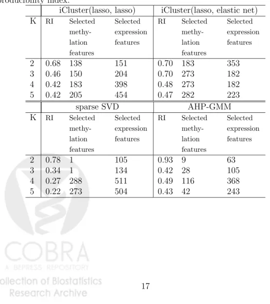
In Table 1, the results from sparse iCluster with two different sets of penalty combina-tions are presented: the combination of (lasso, lasso), and the combination of (lasso, elastic net) for methylation and gene expression data respectively (Table 1 top panel). The re-producibility index (RI) is computed for various Ks and penalty parameters are sampled based on a uniform design described in Section 3.3. As described in Section 5, RI (ranges between 0 and 1) measures the agreement between the predicted cluster membership and the “observed” cluster membership using a 10-fold cross-validation.
Both methods identified a 2-cluster solution with an RI around 0.70, distinguishing the ER-negative, Basal-like subtype from the rest of the tumor samples (Figure 3 and 4, samples labeled in red). The iCluster(lasso, elastic net) method adds anℓ2 penalty term to encourage grouped selection of highly correlated genes in the expression data. This approach further identified a 3-cluster solution with high reproducibility (RI=0.70). The additional division finds a subgroup that highly express platelet-derived growth factor receptors (Figure 4).
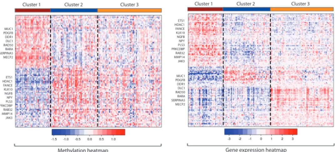
Figure 5 displays heatmaps of the methylation and expression data. Columns are samples ordered by the integrated cluster assignment. Rows are cluster-discriminating genes (with nonzero coefficient estimates) grouped into gene clusters by hierarchical clustering. In total, there are 273 differentially methylated genes and 182 differentially expressed genes. Several cancer genes include MUC1, SERPINA5, RARA, MECP2, RAD50, are hypermethylated
and show concordant underexpression in cluster 1. On the other hand, hypomethylation of several cancer genes including ETS1, HDAC1, FANCE, RAB32, JAK3are hypomethylated and correspondingly show increased expression.
To compare with other methods, we implemented the sparse SVD method by Witten
et al. (2009) and an adaptive hierarchical penalized Gaussian mixture model (AHP-GMM)
by Wang & Zhu (2008) on the concatenated data matrix. None of these methods generated additional insights beyond separating the ER-negative and Basal-like tumors from the others (Figure 3 and Table 1). Feature selection is predominantly “biased” toward gene expres-sion features when directly applying sparse SVD on the combined data matrix (bottom panel of Table 1), likely due to the substantially larger variability observed in gene expression data.
Table 1: Cluster reproducibility and number of genomic feature selected using sparse iClus-ter, sparse SVD on concatenated data matrix, and Adaptive Hierarchically Penalized Gaus-sian Mixture Model (AHP-GMM) on concatenated data matrix. K: the number of clusters. RI: reproducibility index.
iCluster(lasso, lasso) iCluster(lasso, elastic net)
K RI Selected methy-lation features Selected expression features RI Selected methy-lation features Selected expression features 2 0.68 138 151 0.70 183 353 3 0.46 150 204 0.70 273 182 4 0.42 183 398 0.48 273 182 5 0.42 205 454 0.47 282 223 sparse SVD AHP-GMM K RI Selected methy-lation features Selected expression features RI Selected methy-lation features Selected expression features 2 0.78 1 105 0.93 9 63 3 0.34 1 134 0.42 28 105 4 0.27 288 511 0.49 116 368 5 0.22 273 504 0.43 42 243
MUC1 PDGFB DDR1 DLC1 RAD50 RARA SERPINA5 MECP2 ETS1 HDAC1 FANCE KLK10 NGFB NPY PLS3 PRKCDBP RAB32 MMP14 JAK3 ETS1 HDAC1 FANCE KLK10 NGFB NPY PLS3 PRKCDBP RAB32 MMP14 JAK3
Methylation heatmap Gene expression heatmap
MUC1 PDGFB DDR1 DLC1 RAD50 RARA SERPINA5 MECP2
Cluster 1 Cluster 2 Cluster 3 Cluster 1 Cluster 2 Cluster 3
Figure 5: Integrative clustering of the Holm study DNA methylation and gene expression data revealed three clusters with a cross-validated reproducibility of 0.7. Selected genes with negatively correlated methylation and expression changes are indicated to the left of the heatmap.
6.2
Constructing a Genome-wide Portrait of Concordant
Copy-number and Gene Expression Pattern in a Lung Cancer Data
Set
We applied the proposed method to integrate DNA copy number (aCGH data) and mRNA expression data in a set of 193 lung adenocarcinoma samples (Chitale et al., 2009). Figure 6 displays an example of the probe-level data (log-ratios of tumor versus copy number) on chromosome 3 and 8 in one tumor sample. Many samples in this data set display similar chr 3p whole-arm loss and chr 3q whole-arm gain.
Arm-length copy number aberrations are surprisingly common in cancer (Beroukhim
et al., 2010), affecting up to thousands of genes within the region of alteration. A broader
challenge is thus to pinpoint the “driver” genes that have functional roles in tumor develop-ment from those that are functionally neutral (“passengers”). To that end, an integrative analysis with gene expression data could provide additional insights. Genes that show con-cordant copy number and transcriptional activities are more likely to have functional roles. In search for copy number-associated gene expression patterns, we fit a sparse iCluster model for each of the 22 chromosomes using (fused lasso, lasso) penalty combination for joint analysis of copy number and gene expression data. To facilitate comparison, we com-pute a 2-cluster solution with a single latent variable vector z (instead of estimating K) to extract the major pattern for each chromosome. Penalty parameter tuning is performed as described before. In Figure 7, we plot the 22 pairs of the sparse coefficient vectors ordered by chromosomal position. The coefficients can be interpreted as the difference between the
Figure 6: Illustration of copy number probe-level data from a lung tumor sample (Chitale
et al., 2009). Log-ratios of copy number (tumor versus normal) on chromosome 3 and 8 are
displayed. A log-ratio great than zero indicate copy number gain and a log-ratio below zero indicate loss. Black line indicates the segmented value using the circular binary segmentation method (Olshen et al., 2004; Venkatraman & Olshen, 2007).
two cluster means. Positive and negative coefficient values in Figure 7A thus indicate copy number gains and losses in one cluster relative to the other. Similarly, in Figure 7B, coeffi-cient signs indicate over- or under-expression in one cluster relative to the other. Concordant copy number and gene expression changes can thus be directly visualized from Figure 7.
Several chromosomes (1,3, 8, 10, 15 and 16) show contiguous regions of gains or losses spanning whole chromosome arms. As discussed before arm-length aberrations can affect up to thousands of genes within the region of alteration. A great challenge is thus to pinpoint the “driver” genes that have functional roles in tumor development from those that are functionally neutral (“passengers”). To that end, an integrative analysis could provide additional insights. Genes that show concordant copy number and transcriptional activities are more likely to have functional roles. Figure 7 shows that the application of the proposed method can unveil a genome-wide pattern of such concordant changes, providing a rapid way for identifying candidates genes of biological significance. Several arm-level copy number alterations (chromosomes 3, 8, 10, 16) exhibit concerted influence on the expression of a small subset of the genes within the broad regions of gains and losses.
7
Simulation
In this section, we present results from two simulation studies. In the first simulation setup, we simulate a single length-n latent variable z ∼ N(0,1) where n = 100. Subject
j, j = 1,· · · , nbelongs to cluster 1 if zj >0 and cluster 2 otherwise. For simplicity, the pair
of coefficient matrices (W1,W2) are of the same dimension 200×1 (p1 = p2 = 200), with
wi = 3 for i = 1,· · · ,20 for both data type and zero elsewhere. Next we obtain the data
matrices (X1,X2) with each element generated according to equation (1) with standard normal error terms. This simulation represents a scenario where an effective joint analysis of two data sets should be expected to enhance the signal strength and thus improve clustering
Fused Lasso estimates (DNA copy number data) Lasso estimates (mRNA expression data)
A B
Figure 7: Penalized coefficient vector estimates arranged by chromosome 1 to 22 derived by iCluster(fused lasso, lasso) applied to the Chitale et al. lung cancer data set. A single latent variable vector is used to identify the major pattern of each chromosome.
performance.
Table 2 summarizes the performances of each method in terms of the ability to choose the correct number of clusters, cross-validated error rates, cluster reproducibility. In Table 2, separate K-means methods perform poorly in terms of the ability to choose the correct number of clusters, cluster reproducibility, and the cross-validation error rates (with respect to the true simulated cluster membership). K-means on concatenated data performs even worse, likely due to noise accumulation. For sparse SVD, a cluster assignment step is needed. We took a similar approach of applying K-means on the first K−1 right singular vectors of the data matrix. Sparse SVD performs better than simple K-means, though data con-catenation does not seem to offer much advantage. In this simulation scenario, AHP-GMM models show good performance in feature selection (Table 3), but appear to under-estimate the probability of K = 2. A common theme in this simulation is that a data concatenation approach is generally ineffective regardless of the clustering methods used. By contrast, sparse iCluster methods achieved an effective integrative outcome across all performance criteria.
Table 3 summarizes the associated feature selection performance. No numbers are shown for the standard K-means methods as they do not have an inherent feature selection method. Among the methods, sparse iCluster methods perform the best in identifying the true
posi-tive features while keeping the number of false posiposi-tives close to 0.
In the second simulation, we vary the setup as follows. We simulate 150 subjects belong-ing to three clusters (K = 3). Subjectj = 1,· · · ,50 belong to cluster 1, subjectj = 51−100 belong to cluster 2, and subject j = 101,· · · ,150 belong to cluster 3. A total of T = 2 data types (X1,X2) are simulated each has p1 = p2 = 500 features. Here each data type alone only define two clusters out of the three. In data set 1, xij ∼ N(2,1) for i = 1,· · · ,10 and
j = 1,· · · ,50, xij ∼ N(1.5,1) for i = 491,· · ·,500 and j = 51−100, and xij ∼ N(0,1)
for the rest. In data set 2, xij = 0.5∗xij +e where e ∼ N(0,1) for j = 1,· · · ,50 and
i = 1,· · · ,10, xij ∼ N(2,1) for j = 101,· · ·,150 and i = 491,· · ·,500, and xij ∼ N(0,1)
for the rest. The first 10 features are correlated between the two data types. In Table 4 and 5, the sparse iCluster methods consistently performs the best in clustering and feature selection.
7.1
Implementation and running time
The core iCluster EM iterations are implemented in C. Table 3 shows some typical compu-tation times for problems of various dimensions on a 3.2 GHz Xeon Linux computer.
8
Discussion
Integrative genomics is a new area of research accelerated by large-scale cancer genome ef-forts including the Cancer Genome Atlas Project. New integrative analysis methods are emerging in this field. Van Wieringen & Van de Wiel (2009) proposed a nonparametric testing procedure for DNA copy number induced differential mRNA gene expression. Peng
et al.(2010) and Vaskeet al.(2010) considered pathway and network analysis using multiple
genomic data sources. A number of others (Waaijenborg et al., 2008; Parkhomenko et al., 2009; Le Cao et al., 2009; Witten et al., 2009; Witten & Tibshirani, 2009; Soneson et al., 2010) suggested using canonical correlation analysis (CCA) to quantify the correlation be-tween two data sets (e.g., gene expression and copy number data). Most of these previous work focused on integrating copy number and gene expression data, and none of these meth-ods were specifically designed for tumor subtype analysis.
We have formulated a penalized latent variable model for integrating multiple genomic data sources. The latent variables can be interpreted as a set of distinct underlying cancer driving factors that explain the molecular phenotype manifested in the vast landscape of alterations in the cancer genome, epigenome, transcriptome. Lasso, elastic net, and fused lasso penalty terms are used to induce sparsity in the feature space. We derived an efficient and unified algorithm. The implementation scales well for increasing data dimension.
struc-Table 2: Clustering performance summarized over 50 simulated data sets under setup 1 (K=2). Separate clustering methods have two sets of numbers associated with model fit to each individual data type. Number in parentheses is the standard deviation over 50 simulations. Method Frequency of choosing the correct K Cross-validation error rate Cluster Repro-ducibility Separate K-means 58 0.08 (0.04) 0.67 (0.17) 62 0.08 (0.04) 0.70 (0.19) Concatenated Kmeans 50 0.06 (0.04) 0.66 (0.19) Separate sparse SVD 74 0.07 (0.06) 0.71 (0.13) 76 0.07 (0.07) 0.72 (0.12) Concatenated Sparse SVD 78 0.07 (0.08) 0.70 (0.12) Separate AHP-GMM 38 0.06 (0.04) 0.72 (0.15) 40 0.05 (0.04) 0.74 (0.14) Concatenated AHP-GMM 46 0.06 (0.04) 0.75 (0.13) Lasso iCluster 90 0.04 (0.02) 0.81 (0.08) Enet iCluster 94 0.03 (0.02) 0.85 (0.07)
Fused Lasso iCluster 94 0.03 (0.02) 0.83 (0.08)
Table 3: Feature selection performance summarized over 50 simulated data sets for K = 2. There are a total of 20 true features simulated to distinguish the two sample clusters.
Data 1 Data 2
True False True False
Method positives positives positives positives
Separate Kmeans – – – – Concatenated Kmeans – – – – Separate Sparse SVD 18.7 (3.2) 21.5 (37.7) 18.8 (2.9) 27.4 (43.6) Concatenated Sparse SVD 14.0 (5.3) 22.5 (16.1) 13.7 (5.2) 22.8 (16.4) Separate AHP-GMM 19.6 (2.1) 0.02 (0.16) 19.1 (3.1) 0 (0) Concatenated AHP-GMM 18.8 (3.6) 0.02 (0.15) 18.6 (4.0) 0.02 (0.15) Lasso iCluster 20 (0) 0.07 (0.3) 20 (0) 0.07 (0.3) Enet iCluster 20 (0) 0.1 (0.3) 20 (0) 0.02 (0.1)
Table 4: Clustering performance summarized over 50 simulated data sets under setup 2 (K=3). Method Frequency of choosing the correct K Cross-validation error rate Cluster Repro-ducibility Separate K-means 2 0.33 (0.001) 0.54 (0.07) 0 0.33 (0.002) 0.47 (0.04) Concatenated Kmeans 100 0.01 (0.07) 0.96 (0.03) Separate sparse SVD 0 0.28 (0.10) 0.45 (0.03) 0 0.31 (0.07) 0.44 (0.04) Concatenated Sparse SVD 16 0.01 (0.002) 0.59 (0.05) Separate AHP-GMM 0 0.07 (0.13) 0.63 (0.05) 0 0.32 (0.02) 0.54 (0.06) Concatenated AHP-GMM 100 0.01 (0.07) 0.98 (0.03) Lasso iCluster 100 0.0003 (0.001) 0.98 (0.01) Enet iCluster 100 0.0003 (0.001) 0.97 (0.02)
Fused Lasso iCluster 100 0 (0) 0.94 (0.05)
Table 5: Feature selection performance summarized over 50 simulated data sets underK = 3.
Data 1 Data 2
True False True False
Method positives positives positives positives
Separate Kmeans – – – – Concatenated Kmeans – – – – Separate Sparse SVD 19.8 (0.7) 349.6 (167.1) 19.9 (0.3) 347.5 (142.5) Concatenated Sparse SVD 20 (0) 396.6 (128.7) 19.6 (1.6) 395.4 (128.3) Separate AHP-GMM 15.8 (5.0) 239.9 (245.5) 15.5 (5.5) 269.9 (246) Concatenated AHP-GMM 19.2 (1.7) 0.33 (0.64) 14.4 (4.0) 0.21 (0.66) Lasso iCluster 20 (0) 1.5 (1.4) 19.9 (0.2) 1.9 (1.5) Enet iCluster 20 (0) 0.5 (0.6) 19.8 (0.5) 0.7 (1.0)
Table 6: Computing time (in seconds) for typical runs of sparse iCluster under various dimension.
Time (in seconds)
p N Lasso iCluster Elasticnet iCluster Fused Lasso iCluster
200 100 0.10 0.11 0.37
500 100 0.50 0.36 3.56
1000 100 1.40 1.45 25.05
2000 100 6.49 5.90 76.40
5000 100 18.93 18.94 33 (min)
ture defined a priori. Two types of group structures are relevant for our application. One is to treat the wi1,· · · , wi(K−1) as a group since they are associated with the same feature. Yuan and Lin’s group lasso penalty Yuan & Lin (2006) can be applied directly. Similar to our current algorithm, by using Fan and Li’s local quadratic approximation, the problem reduces to a ridge-type regression in each iteration. The other extension is to incorporate the grouping structure among features to boost the signal to noise ratio, for example, to treat the genes within a pathway as a group. We can consider a hierarchical lasso penalty (Wang et al., 2009) to achieve sparsity at both group level and individual variable level.
References
Alizadeh, A. A., Eisen, M. B., Davis, E. E.,et al.(2000).Nature, 403, 503–511.
Beroukhim, R., Mermel, C.H. Porter, D., Wei, G., Raychaudhuri, S., Donovan, J., Barretina, J., Boehm, J., Dobson, J., Urashima, M., Mc Henry, K., Pinchback, R., Ligon, A., Cho, Y., Haery, L., Greulich, H., Reich, M., Winckler, W., Lawrence, M., Weir, B., Tanaka, K., Chiang, D., Bass, A., Loo, A., Hoffman, C., Prensner, J., Liefeld, T., Gao, Q., Yecies, D., Signoretti, S., Maher, E., Kaye, F., Sasaki, H., Tepper, J., Fletcher, J., Tabernero, J., Baselga, J., Tsao, M., Demichelis, F., Rubin, M., Janne, P., Daly, M., Nucera, C., Levine, R., Ebert, B., Gabriel, S., Rustgi, A., Antonescu, C., M., L., Letai, A., Garraway, L., Loda, M., Beer, D., True, L., Okamoto, A., Pomeroy, S., Singer, S., Golub, T., Lander, E., Getz, G., Sellers, W., & Meyerson, M. (2010).Nature, 463, 899–905.
Carvalho, I., Milanezi, F., Martins, A., Reis, R., & Schmitt, F. (2005).Breast Cancer Research, 7, R788–95.
Chen, H., Xing, H., & Zhang, N. (2011).PloS computational biology, 7, 1–15.
Chin, L. & Gray, J. (2008).Nature, 452, 553–563.
Chitale, D., Gong, Y., Taylor, B., Broderick, S., Brennan, C., Somwar, R., Golas, B., Wang, L., Motoi, N., Szoke, J., Reinersman, J., Major, J., Sander, C., Seshan, V., Zakowski, M., Rusch, V., Pao, W., Gerald, W., & Ladanyi, M. (2009).Nature, 28(31), 2773–83.
Dempster, A. P., Laird, N. M., & Rubin, D. B. (1977). Journal of the Royal Statistical Society: Series B (Statistical Methodology),
39, 1–38.
Dudoit, S. & Fridlyand, J. (2002). Genome Biology, 3(7), 1–21.
Fan, J. & Li, R. (2001). Journal of the American Statistical Association, 96, 1348–1360.
Fang, K. & Wang, Y. (1994). Number theoretic methods in statistics.London, UK: Chapman abd Hall.
Feinberg, A. & Vogelstein, B. (1983). Nature, 301, 89–92.
Hastie, T., Tibshirani, R., & Friedman, J. (2009). The Elements of Learning: Data Mining, Inference, and Prediction. New York, NY: Springer.
Holliday, R. (1979).Br J Cancer, 40, 513–22.
Holm, K., Hegardt, C., Staaf, J.,et al.(2010).Breast Cancer Research, 12, R36.
Hoshida, Y., Nijman, S., Kobayashi, M., Chan, J., Brunet, J., Chiang, D., Villanueva, A., Newell, P., Ikeda, K., Hashimoto, M., Watanabe, G., Gabriel, S., Friedman, S., Kumada, H., Llovet, J., & Golub, T. (2003).Cancer Research, 69, 7385–92.
Irizarry, R., Ladd-Acosta, C., Carvalho, B., Wu, H., Brandenburg, S., Jeddeloh, J., Wen, B., & Feinberg, A. (2008).Genome Research,
18, 780–90.
Jolliffe, I. T. (2002). Principal Component Analysis. New York, NY: Springer.
Kapp, A. & Tibshirani, R. (2007).Biostatistics, 8, 9–31.
Laird, P. (2003). Nat Rev Cancer, 3, 253–66.
Laird, P. (2010). Nat Rev Genet, 11, 191–203.
Lapointe, J., Li, C., Higgins, J., van de Rijn, M., Bair, E., Montgomery, K., Ferrari, M., Egevad, L., Rayford, W., Bergerheim, U., Ekman, P., DeMarzo, A., Tibshirani, R., Botstein, D., Brown, P., Brooks, J., & Pollack, J. (2003). Proceedings of the National Academy of Sciences, 101, 811–6.
Le Cao, K., Martin, P., & Robert-Granie, C. abd Besse, P. (2009). BMC Bioinformatics, 26, 34.
Ng, A., Jordan, M., & Weiss, Y. (2002). Advances in neural information processing systems, 2, 849–56.
Olshen, A., Bengtsson, H., Neuvial, P., Spellman, P., Olshen, R., & Seshan, V. (2011).Bioinformatics, 27, 2038–46.
Olshen, A., Venkatraman, E., Lucito, R., & Wigler, M. (2004). Biostatistics, 5(4), 557–572.
Peng, J., Zhu, J., Bergamaschi, A., Han, W., Noh, D., Pollack, J., & Wang, P. (2010). Annals of Applied Statistics, 4, 53–77.
Perou, C. M., Jeffrey, S. S., van de Rijn, M.,et al.(1999).Proceedings of the National Academy of Sciences, 96, 9212–9217.
Pollack, J. R., Sørlie, T., Perou, C. M.,et al.(2002).Proceedings of the National Academy of Sciences, 99, 12963–12968.
Rohe, K., Chatterjee, S., & Yu, B. (2010).ArXiv e-prints, .
Sharpless, N. E. (2005). Mutat. Res.576, 99–102.
Shen, R., Olshen, A., & Ladanyi, M. (2009).Bioinformatics, 25(22), 2906–2912.
Simon, R. (2010). Expert Reviews Molecular Medicine, 12(e23).
Soneson, C., Lilljebjrn, H., Fioretos, T., & Fontes, M. (2010). BMC Bioinformatics, 11, 191.
Sorlie, T., Perou, C. M., Tibshirani, R.,et al.(2001).Proceedings of the National Academy of Sciences, 98, 10869–10874.
TCGA Network (2008). Nature, 455, 1061–1068.
TCGA Network (2011). Nature, 474, 609615.
Tibshirani, R. (1996).Journal of the Royal Statistical Society: Series B (Statistical Methodology), 58, 267–288.
Tibshirani, R., Saunders, M., Rosset, S., Zhu, J., & Knight, K. (2005).Journal of the Royal Statistical Society Series B.67, 91–108.
Tibshirani, R. & Walther, G. (2005).Journal of Computational & Graphical Statistics, 14(3), 511–528.
Tibshirani, R. & Wang, P. (2008).Biostatistics, 1(9), 18–29.
Van Wieringen, W. & Van de Wiel, M. (2009). Biometrics, 65, 19–29.
Vaske, C., Benz, S., Sanborn, J., Earl, D., Szeto, C. Zhu, J., Haussler, D., & J.M., S. (2010). Bioinformatics, 26, 237–45.
Venkatraman, E. S. & Olshen, A. B. (2007).Bioinformatics, 23(6), 657–663.
Waaijenborg, S., Verselewel de Witt Hamer, P. C., & Zwinderman, A. H. (2008). Statistical Applications in Genetics and Molecular Biology, 7, Article 3.
Wang, S., Nan, B., Zhu, J., & Beer, D. (2008).Biometrics, 64, 132–140.
Wang, S., Nan, B., Zhu, N., & Zhu, J. (2009). Biometrika, 96(2), 307–322.
Wang, S. & Zhu, J. (2008).Biometrics, 64, 440–448.
Witten, D. M. & Tibshirani, R. (2009).Statistical Applications in Genetics and Molecular Biology, 8(1), Article 28.
Witten, D. M., Tibshirani, R., & Hastie, T. (2009).Biostatistics, 10, 515–534.
Yuan, M. & Lin, Y. (2006). Journal of the Royal Statistical Society (Series B), 68, 49–67.