MODELING THE EFFECTS OF LOW IMPACT DEVELOPMENT PRACTICES
ON STREAMS AT THE WATERSHED SCALE
A Dissertation by
SA’D ABDEL-HALIM SA’D-EDDIN SHANNAK Submitted to the Office of Graduate and Professional Studies of
Texas A&M University
in partial fulfillment of the requirements for the degree of DOCTOR OF PHILOSOPHY
Chair of Committee, Patricia Smith Co-Chair of Committee, Fouad Jaber Committee Members, Ronald Kaiser
Jacqueline A. Peterson Roger Glick
Indisciplinary Faculty
Chair, Ronald Kaiser
May 2014
Major Subject: Water Management and Hydrological Science
ii
ABSTRACT
Urban growth contributes to increasing stormwater runoff which in turn causes an increase in the frequency and severity of flooding. Moreover, increased stormwater runoff contributes to changing the character and volume of energy inputs to the stream. Traditionally, stormwater management controls such as detention pond had been extensively studied and evaluated with respect to reducing and controlling peak flows. Nonpoint source pollutants due to urbanization and expanding of agricultural fields have become a big burden on municipalities and states.
Low Impact Development practices were developed to negate the negative impacts of urbanization on water resources by reducing the runoff volume and peak flows as well as improving outflow water quality. Though these practices have the capability of
reducing runoff volumes and enhancing outflow water quality, they can be costly. Therefore, understanding the impact of installing LID practices on a watershed scale is becoming increasingly important.
In this study, field experiment and model study were applied to evaluate the effectiveness of LID practices on a watershed scale in the Blunn Creek Watershed located in Austin, Texas. The three LID practices which were evaluated in this study are permeable pavements, a bioretention area, and a detention pond. The main objective of this study was to investigate the influences of these practices at a watershed scale on: potential reduction on channel bank erosion, potential reduction on flood, and potential impact on aquatic life.
iii
This study was one of very few studies that take place in the Blackland clay soil in Texas. A combination of different levels of LID practices such as permeable
pavement and bioretention area resulted with achieving the main goal of this study of reducing stream bank erosion, bankfull exceedance, and maintaining acceptable flows for the integrity of aquatic life habitat. All LID practices have shown significant difference with respect to a control treatment at 95% confidence ratio. Performance of the modeled LID practices was validated by showing acceptable agreement in the percentage of reductions in total runoff between field experiments and model data.
iv
DEDICATION
v
ACKNOWLEDGEMENTS
My first and most earnest gratitude goes to the Almighty Allah for materializing my dream. I would like to acknowledge my research advisor Dr. Fouad Jaber, and my research committee members for their inspiring, helpful suggestions and persistent encouragements as well as close and consistent supervision throughout the period of my Doctoral program. Dr. Jaber has provided insightful discussions about the research. I am also very grateful for his scientific advice and knowledge and many insightful
discussions and suggestions.
This work wouldn’t be possible without the support and contributions of many people. I would like to thank the staff members of the watershed protection department at City of Austin. I thank Roger Glick and Leila Gosselink for their help providing data and support through my research work.
Again, many thanks to Dr. Jaber for all the support and for getting all my science questions answered.
Most of all, I thank my parents, my wife, and kids for their loving support through my life.
vi TABLE OF CONTENTS ABSTRACT ... ii DEDICATION... iv ACKNOWLEDGEMENTS ... v TABLE OF CONTENTS ... vi LIST OF FIGURES ... ix LIST OF TABLES ... xi CHAPTER I INTRODUCTION ... 1 Literature Review ... 2
Channel Response to Development-Induced Watershed Changes ... 3
Urbanization and Aquatic-System Degradation ... 5
Urbanization and Flood Frequency ... 7
Goal and Objectives ... 10
CHAPTER II CALIBRATION AND EVALUATION OF SWAT FOR SUB-HOURLY TIME STEPS ... 12
Synopsis ... 12 Introduction ... 13 Model Description... 17 SWAT... 17 SWAT_CUP ... 19 Methodology ... 21 SWAT-CUP Setup ... 21 Calibration Parameters ... 23 Uncertainty Analysis ... 24 Case Study ... 25 Results ... 28 Conclusions ... 37
CHAPTER III MODELING STREAM BANK EROSION AT A WATERSHED SCALE IN THE BLACKLAND PRAIRIE ECOSYSTEM ... 39
Synopsis ... 39 Page
vii
Introduction ... 40
Erosion and Hydrological Modeling ... 43
Stream Stability... 45
Methodology ... 48
Model Development ... 48
Calibration and Validation ... 49
Sensitivity Analysis... 50
Channel Geometry and Hydraulic Properties ... 51
LIDs Development and Representation ... 54
Detention Pond Development ... 55
Bioretention/Raingarden and Permeable Pavement Development and Representation ... 57
Potential Erosion Estimates ... 60
Cost Analysis ... 62
Statistical Analysis ... 63
Performance Validation of LIDs... 63
Results ... 65
Sensitivity Analysis ... 66
Model Calibration and Validation ... 68
Channel Geometry and Hydraulic Properties ... 69
Potential Erosion Estimates ... 70
Cost Analysis ... 76
Statistical Analysis ... 77
Performance Validation of LIDs ... 79
Conclusions ... 80
CHAPTER IV LOW IMPACT DEVELOPMENT RESPONSE TO URBANIZATION AND FLOODING SIMULATED BY SUB-HOURLY SWAT MODEL IN THE BLUNN CREEK WATERSHED ... 81
Synopsis ... 81
Introduction ... 82
Methodology ... 86
Model Setup ... 86
Data Acquisition ... 88
Model Calibration and Validation ... 89
LID Representation in SWAT ... 91
Flood Impacts ... 94
Results and Discussion ... 97
Performance Validation ... 106
Conclusions ... 107
CHAPTER V EFFECT OF URBANIZATION ON AQUATIC-SYSTEM DEGRADATION ... 109
viii
Synopsis ... 109
Introduction ... 110
Methodology ... 114
Input Data ... 116
Potential Aquatic Life Evaluation ... 117
Results ... 120
Conclusions ... 122
CHAPTER VI OVERALL CONCLUSIONS ... 124
CHAPTER VII RECOMMENDATIONS FOR FUTURE STUDIES ... 128
REFERENCES ... 129 Page
ix
LIST OF FIGURES
Figure 2-1. Interaction between calibration program and SWAT in SWAT-CUP
(Abbaspour, 2007) ... 20
Figure 2-2. Screen shot of Sub-hourly saveconc command ... 22
Figure 2-3. Blunn Creek Watershed in Austin, Texas. ... 26
Figure 2-4. Cross section analysis for the DEM layer using 3D Analyst tool. ... 27
Figure 2-5. Global sensitivity analysis for an initial run that accounts for all uncertainty parameters ... 29
Figure 2-6. Sensitive parameters during sub-hourly calibration for the Blunn Creek Watershed vs. objective function. a: Threshold depth of water in the shallow aquifer required for return flow to occur, b: Soil evaporation compensation factor, c:Available water capacity of the soil layer, d: Saturated hydraulic conductivity, e: Groundwater delay, f: Base flow alpha factor, g: Manning roughness for main channel, h: Effective hydraulic conductivity ... 31
Figure 2-7. Initial iteration with all available parameters ... 34
Figure 2-8. Iteration accounts for parameters with the highest sensitivity level ... 35
Figure 3-1. Example of HEC-RAS analysis ... 53
Figure 3-2. Example of WinXSPRO analysis ... 54
Figure 3-3. Location of a Detention Pond at subbasin 10 ... 56
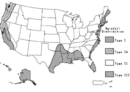
Figure 3-4. Geographic boundaries for SCS rainfall distribution (Asquith and Roussel, 2004) ... 57
Figure 3-5. Schematic of Austin sedimentation/filtration basins [Courtesy of City of Austin (2011)]: (a) configuration of full/partial sedimentation filtration basins; (b) riser pipe outlet system and flow spreader in full type systems ... 58
Figure 3-6. Example of a bioretention/raingarden sizing ... 60 Page
x
Figure 3-7. Shear stresses (lbs. square feet) for current scenario and different levels of LIDs based on Sedfil modification. ... 71 Figure 3-8. Excess shear for the current scenario without LIDs ... 72 Figure 3-9. Annual excess shear (Pa) for different development densities and
median soil particle size equivalent to 20 mm... 76 Figure 4-1. Land use map for Blunn Creek Watershed (current scenario) ... 89 Figure 4-2. Cross section analysis of Blunn Creek Watershed using HEC-RAS
software ... 94 Figure 4-3. Stage discharge analysis for Blunn Creek using HEC-RAS software ... 95 Figure 4-4. Peak discharges reduction (%) by adding RG only for different design
storms ... 98 Figure 4-5. Peak discharges reduction (%) by adding RG and PP for different design
storms ... 99 Figure 4-6. Peak discharges reduction (%) by adding RG and PP for different design
storms ... 100 Figure 4-7. Peak discharges reduction (%) by adding PP only for different design
storms ... 101 Figure 4-8. Percentage of exceedance reduction (%) of bankfull discharge by adding
PP only for different design storms and for all subbasins ... 103 Figure 4-9. Percentage of exceedance reduction (%) of bankfull discharge by
adding RG only for different design storms and for all subbasins ... 104 Figure 4-10. Percentage of exceedance reduction (%) of bankfull discharge by
adding DP only for different design storms and for all subbasins ... 105 Figure 4-11. Percentage of exceedance reduction (%) of bankfull discharge by
combining PP and RG for different design storms and for all subbasins . 106 Figure 5-1. Logical model of the study ... 116 Figure 5-2. Percentage of AQP value increase when utilizing LID practices. ... 120 Figure 5-3. The effect of LID practices on increasing baseflow. ... 121 Page
xi
LIST OF TABLES
Table 2-1. Initial calibration parameters given by SWAT-CUP ... 23
Table 2-2. Stream flow parameters selected for calibration ... 28
Table 2-3. Parameter sensitivities for SUFI-2 ... 30
Table 2-4. Stream flow calibration parameter uncertainties ... 30
Table 2-5. Stream flow calibration results for sub-hourly model... 34
Table 2-6. Average annual water balance components and error percentages for the calibration period at the Blunn Creek Watershed ... 36
Table 3-1. Median soil particle sizes and classification used in potential erosion estimates (Julien, 1995) ... 61
Table 3-2. Monitoring system and equipment used to report LIDs performance at the Texas A&M Agrilfe Extension Services Center in Dallas Texas. ... 65
Table 3-3. Stream flow parameters selected for calibration ... 67
Table 3-4. Parameter sensitivities for SUFI-2 ... 67
Table 3-5. Stream flow calibration results for sub-hourly model... 68
Table 3-6. Median soil particle sizes and corresponding critical shear stress at each subbasin in the Blunn Creek Watershed ... 69
Table 3-7. Reduction percentages in excess shear stress for different soil particle diameters and by utilizing different types of LID practices. ... 73
Table 3-8. Reduction percentages in runoff volumes and peak flows for different recurrence intervals and by utilizing different types of LID practices. ... 74
Table 3-9. Total cost of the studied LIDs ... 77
Table 3-10. Summary t-Test: Paired Two Sample for Means Current and LID practices ... 77
xii
Table 4-1. Hydrological characteristics of Blunn Creek Watershed ... 96 Table 4-2. Recurrence intervals and equivalent rainfall amounts ... 97 Table 4-3. Eceedance percentages of the current scenarios without LIDs ... 102 Table 4-4. Comparison of LID performance between field experiment and model
data... 107 Page
1
CHAPTER I
INTRODUCTION
Urban areas are expanding rapidly in the United States, resulting in an increase in impervious cover (EPA, 2012).Urban growth contributes to increasing stormwater runoff which in turn causes an increase in the frequency and severity of flooding. Moreover, increased stormwater runoff contributes to changing the character and volume of energy inputs to the stream. As a result, infiltration and base flow, as a proportion of total flow, will decrease and urban runoff volumes, frequency of flooding and peak runoff flow rates will increase (EPA, 2012). The consequences of urbanization will be reflected not only in the hydrological cycle and infrastructure, but also in human health and
environment. Urban runoff has a significant role in transporting pollutants such as chemicals, sediments, pesticides, fertilizers, and oils into water bodies, where they harmfully affect water quality (Kim et al., 2007; Davis, 2007).
Low Impact Development (LID) practices were developed to reduce the negative impacts of urbanization on water resources by reducing runoff volumes and peak flows as well as improving outflow water quality (Villarreal et al., 2004). LID practices include the installation of any of the following structural measures to retrofit existing infrastructure and to reduce runoff volumes and peak flows; bioretention, green roofs, rainwater harvesting, and permeable pavements (Damodaram, 2010). LID practices has gained popularity because of their role in maintaining post development hydrograph close to the natural condition present before development occurs (Coffman 2002). The installation of these practices contributes to decreasing the need for paving, gutters,
2
curbs, and inlet structures that eventually reduce the infrastructure construction and maintenance costs (Sample et al., 2002). Previous studies confirmed the beneficial uses of LID practices at the micro-scale such as plot or small field experiment in comparison to developed scenario without any consideration to LID structures (Selbig and
Bannerman 2008; Bedan and Clausen 2009; Wang et al. 2010; Zimmerman et al. 2010). However, there is still many discussions and debates about many of these practices and their benefits on larger scales such as watershed scale. Therefore, understanding the impact of installing LID practices on a watershed scale is becoming increasingly important.
Literature Review
Increasing impervious cover through urbanization will lead to an increase in runoff volumes, and eventually this will increase flooding. Stream channels adjust by widening and eroding stream banks which can impact downstream properties negatively (Chin and Gregory, 2001). Also, urban runoff drains through sediment bank areas, known as riparian zones, and constricts stream channels (Walsh, 2009). Physical and chemical factors associated with urbanization such as high peak flows and low water quality stress aquatic life and contribute to the overall biological condition of urban streams (Maxted et al., 1995). While LID practices have been mentioned and studied in literature for stormwater management, they have not been studied in respect to reducing potential impact on flooding, stream bank and bed erosion and aquatic life.
To better evaluate the performance and the effectiveness of LID practices at a watershed scale, three practices were introduced (sustainable detention pond,
3
bioretention, and permeable pavement). These practices capture the storm and base flow over a longer period of time, and are recommended as new metrics to characterize the magnitude of urban development influence, stream bank and bed erosion, aquatic life, and flood. These measures will create a linkage between urban watershed development and stream conditions in particular biological health.
Channel Response to Development-Induced Watershed Changes
Changing land uses due to urbanization can have harmful effects on urban and suburban streams, both hydrologically and biologically. Impervious surfaces generate higher peak flows which cause stream enlargement through bed and bank erosion (Ludwig et al., 2005; Sovern and Washington, 1997). The channel erosion observed in streams surrounded by urbanized areas is due to the increased frequency of the bankfull discharge (Pizzuto et al., 2000). Bankfull discharge reflects a state of maximum velocity in the channel, and therefore maximum competence for the transport of the load. It is generally accepted to be the dominant discharge that is close to steady- state conditions (Carling, 1988). Bankfull flows occur only every one to two years in a pristine stream (Leopold, 1994). Though, with the impact of urban development these flows can occur three to five (Klein, 1979, Booth, 1991) times per year, causing bank erosion, movement of large woody debris, and infilling of pools (Booth, 1991). Streams continue to enlarge until water velocity drops to a stable level which is defined as stream equilibrium and reaching this stable level might be delayed for several decades based on the additional volumes of flows received (Morisawa and LaFlure, 1979).
4
Numerous studies link the influence of urbanization and stream health and enlargement due to bank and bed erosion (Goodwin et al., 1997). Hession et al., (2003) studied the influence of varying riparian vegetation on channel morphology in rural and urban watersheds. They found that channel width and cross-sectional area are larger in urban watersheds and documented a significant difference of (p<0.001). Also, bankfull channels in forested streams are wider and have greater cross-sectional areas, while there are no significant differences between forested and non-forested bankfull depth,
sinuosity, slope, or median bed particle size (Hession et al., 2003). Trimble (1997) conducted a study to evaluate the contribution of stream channel erosion to sediment yield from an urbanizing watershed. The study considered San Diego Creek in southern California, and measurements from 1983 to 1993. Results showed that stream channel erosion provided 105 Mg/yr of sediment, or about two-thirds of the total sediment yield. Another study conducted by Bledsoe and Watson (2001) found that even low levels of imperviousness 10 to 20 % have the potential to destabilize urban streams. On the other hand, Wolman and Schick (1976) found that some morphological changes and
adjustments in urban streams are not strictly responses to altered stream flow patterns. For instance, banks that have been defrosted or artificially stabilized can have narrower channels and this change was not inherited from alteration in stream flow.
Konrad et al., (2005) studied the impact of urban development on stream flow and streambed stability. They examined 16 streams in the Puget Lowland, Washington, using three stream flow metrics that integrate storm-scale effects of urban development over annual to decadal timescale. They concluded that the increase in the magnitude of
5
frequent high flows due to urban development but not their cumulative duration has important consequences for channel form and bed stability in gravel bed streams. That can be explained by the geomorphic equilibrium which depends on moderate duration. Streams with low values of TQmean (fraction of time that stream flow exceeds the mean stream flow) and T0.5 (fraction of time that stream flow exceeds the 0.5-year flood) are narrower than expected from hydraulic geometry (Konrad et al., 2005). At this point, creating different development scenarios and applying several levels of LID practices is becoming increasingly important to better evaluate the performance of LID practice at a watershed scale. The available literature concluded that urbanization increases the magnitude of frequent high flows and all the negative impact associated with it, but none of the available literature projected the effect of future urban development scenarios (with LID practices with respect to human health and environment).
Urbanization and Aquatic-System Degradation
Stream ecosystems are the most fragile, degraded, and threatened ecosystems because of the strong interactions between aquatic and terrestrial environments and human disturbances that can affect either system (Nature Conservancy, 1996). Changes in demographic and land use due to urbanization have brought about profound changes to the physical, chemical, and biological integrity of streams (Hollis, 1975). Variation in flow over a day and a season can affect aquatic life (May, 1997). Low base flows during summer and dry periods can cause fish mortalities due to reduced velocity,
cross-sectional area, and water depth (Williamson et al., 1993). Also, high flows can wash salmonid eggs from reeds (Vronskii and Leman, 1991). While high flows can be
6
essential to help in the migration of all fish when water velocity exceeds their swimming speed, juveniles are more vulnerable to high flows (Chilibeck et al., 1993). Moreover, high water velocity due to urbanization can be extremely harmful to the stream
environment if there is a lack of boulders and large woody debris, which provide eddies where fish can rest and have shelter. Rood and Hamilton (1994) found out that Salmon habitat had a significant degradation over the past one hundred years due to altering flow regimes and removal of riparian vegetation. Klein (1979) concluded that when
watershed imperviousness exceeds 10 percent, a rapid decline in biotic diversity might result. Sovern and Washington (1997) concluded that urbanization causes an increase in sediment load due to stream enlargement through bed and bank erosion. These additional volumes of sediment loads contribute to clogging and degrade salmonid spawning gravel quality by reducing the gravel porosity, hence hindering the resupply of dissolved
oxygen to fish eggs. Reed (1978) conducted a study in the state of Pennsylvania where he looked at the effectiveness of sediment-control techniques during highway
construction in respect to aquatic life. Results showed that suspended sediments coming from construction activities can harmfully affect aquatic life by habitat elimination under heavy loading or by interference with feeding under lighter stress. Whipple et al. (1981) concluded in their study that the decrease in low flow discharges eliminates the available stream habitat, increases the probability that the streams may go dry, may increase temperature fluctuations and increase the concentration of pollutants due to lack of dilution which in its turn negatively reflects on aquatic life health. DeGaspari et al. (2009) utilized hydrologic modeling to emulate hydrologic metrics for different
7
development scenarios. The aim of the study was to determine which development scenario best met management plans with respect to aquatic life. Though this was found to be a suitable method, hydrologic metrics which can be reliably predicted by the model should be selected over other metrics that cannot be predicted well.
All previous literature studied the influence of urbanization, landuse, variability of flow, and suspended solids due to bed and bank erosion on aquatic life, there is a great need for modeling the effect of LID practices at a watershed scale on aquatic life. Most of the available research considered metrics that were poorly suited to characterize the magnitude of hydrological changes and their impact on biological stream health. Modeling the impact of change in hydrology due to urbanization based on field data on aquatic life is becoming very important.
Urbanization and Flood Frequency
Urban development contributes to modify hydrological processes when
vegetation cover and soil are cleared from the land surface (Jones and Clark, 1987). The more the impervious cover the higher the flood frequencies that may result (Moscrip and Montgomery, 1997). Poff and Ward (1989) studied daily flow records for seventy eight USGS stations across the United States for variability and the pattern of the flood regime. They characterized streams into different classes by their hydrologic characteristics and these that could theoretically have an impact on the biological community and flood frequencies. They were unable to quantitatively relate stream biology to hydrology due to the lack of consistent data. Another study by Scoggins (2000) proved that hydrologic parameters proposed by both Poff and Ward (1989) might
8
be used to characterize streams in central Texas and that these parameters might be related to stream biology and flood frequency. Olden and Poff (2003) tested the
redundancy in proposed hydrologic indices using the same sites used by Poff and Ward (1989). They concluded that many of the 171 hydrologic indices tested were correlated and redundancy could be reduced by using principal component analysis to reduce collinearity. Moscrip and Montgomery (1997) studied six low-order streams in the Puget Lowlands, Washington, for the period between the 1940-1950 and the 1980-1990. They utilized USGS station records and each basin was separated into periods prior to and after urban expansion. Results showed that each basin that experienced a significant increase in urbanized areas showed increased flood frequency. The pre-urbanization 10-year recurrence interval flows correspond to 1 to 4-10-year recurrence interval events in post-urbanization records. On the other hand, no apparent shift in flood frequency was observed in either of the control basins that represent a limited change in the urbanized area. Schueler (1992) concluded that urbanization alters stream hydrology and increases stream velocity, flooding magnitude, and flooding frequency. Also, flood duration typically declines as the time from peak to base flow discharge is reduced (Paul and Meyer, 2001). Hirsch et al., (1990) showed that flood duration depends on the degree of urbanization, spatial management and location of impervious cover within the basin.
Although the effects of urbanization on watershed hydrology and river-channel morphology have been studied for decades as literature mentioned above showed, previous studies focused on a limited number of morphologic variables and ignored the complicating influence of varying LID practices types and designs. There is still a great
9
need to evaluate these controls in the field and to collect quantitative data to evaluate their performance, especially in the Southern part of the United States. There is also very little data on the potential impact of the adoption of LID practices at a watershed level. Sample and Heaney (2006) stated that the lack of such research is caused by the
difficulty of modeling processes at the small scale required by low impact development (LID) management options without field data. There are very few research that studied the effectiveness of LID practices and their performance based on field data with respect to reducing potential impact on flooding, stream bank and bed erosion and aquatic life. None of the available research studied the correlation between changing in the
hydrology on a watershed scale due to urbanization after the installation of LID practices (sustainable detention pond, bioretention and permeable pavement) and potential impact on flooding, stream bank and bed erosion, and aquatic life.
Most of the available studies evaluate the effectiveness of LID practices on a site scale using field experiments, modeling or by developing algorithms based on design storms or average rainfall Graham et al., 2004). Several efforts contribute to analyze the effectiveness of these practices based on pollutant removal such as nitrogen, phosphorus and total fecal (Hunt et al., 2008). Other studies focused on the cost effectiveness
incentives of LID practices solely (EPA, 2014). Bracmort et al. (2006) studied the effectiveness of LID practices over the long term in respect to enhancing water quality. They ran several scenarios using Soil and Water Assessment Tool (SWAT) to determine the long term (20 years) impact of LID practices on water quality for two watersheds. Results showed that LID practices that were in a good condition (regularly maintained)
10
reduced the average annual sediment yield by 16% to 32% and the average annual phosphorus yield by 10% to 24%. On the other hand, LID practices in their current condition reduced sediment yield by 7% to 10% only and phosphorus yield by 7% to 17%.
There are very few studies that address the effectiveness of LID practices at a watershed scale. There is a great need to understand the functionality of these practices, their ability to adjust the changes in land uses, and return peak flows to the
pre-development scenario.
The hypothesis of this research study is that the integration of LID practices at watershed scale improves stream health and conditions. Specifically:
1) LID practices reduce potential bed stream erosion in urban areas 2) LID practices provide healthy environment for aquatic life habitat 3) LID practices reduce potential flooding in urban streams
This study is one of very few studies that took place in the Blackland clay soil in Texas. Blackland clay soil consists of about 12.6 million acres of east-central Texas extending southwesterly from the Red River to Bexar County, which covers mostly the biggest cities in Texas; Austin, Dallas, San Antonio, and Houston (Texas Almanac, 2013).
Goal and Objectives
The main goal of this study is to evaluate and model the effects of LID practices /green building infrastructure on streams at a watershed scale. The three LID practices
11
targeted in this study are permeable pavements, a bioretention area, and a detention pond. The specific objectives of this research are to investigate the influences of LID practices at a watershed scale on:
Potential reduction on channel bank erosion , Potential reduction on flood and
12
CHAPTER II
CALIBRATION AND EVALUATION OF SWAT FOR SUB-HOURLY
TIME STEPS
Synopsis
SWATis a semi-distributed, lumped parameter, river basin scale, continuous time model that was developed to simulate hydrology and water quality in watersheds. Traditionally, the model operated at a daily time step and it estimated the influence of landuse and management practices on water, agricultural chemical yields in a watershed. The daily time step format provided by SWAT may not be sufficient to capture the impact of flashy storms where peak flows last for minutes only and are not reflected in daily average flows. It might also miss important processes such as the first flush of urban runoff. A sub-hourly model for urban applications was developed by Jeong and Srinivasan (Jeong et al., 2010) but is currently not widely used. SWAT-CUP is a calibration program that is interfaced with SWAT. The main goal of this study was to apply sub-hourly time steps using SWAT and SWAT CUP to calibrate these sub-hourly models. The model was tested using data from the Blunn creek watershed in Austin, TX.
This study presents the calibration and evaluation process and examines
uncertainty using the sequential uncertainty fitting (SUFI-2) method in SWAT-CUP for a sub-hourly 15-minute time step model. The model was calibrated and evaluated for a 2- year period. Results show that the sub-hourly SWAT model provides reasonable estimates of stream flow for multiple storm events. Calibrated stream flows for a 2 year period using the 15- minute time step had an R2 of 0.78 and a Nash-Sutcliff coefficient
13
(NS) of 0.78. The P-factor and R-factor calculated using SUFI-2 procedures have provided good agreement by bracketing around 54- 56% observed data on a sub-hourly basis. The 2 year validation period had an R2 of 0.70 and a NS of 0.67. It was concluded that the sub-hourly SWAT in conjunction with SWAT-CUP have the capabilities to simulate and estimate parameter uncertainty for complex hydrological processes and their interactions.
Introduction
Most hydrological models must be calibrated so their outputs can be used for tasks ranging from regulation to research (EPA, 2002). Distributed hydrological models often account for several variables that include data from numerous fields; weather, soil, land use, surface and ground water and management practices. Manual calibration is difficult due to the complexity of large scale models with many objectives and the numerous interactions between these objectives (Abbaspour et al. 2007). The process of calibration accounts for testing a model using known inputs and outputs data to closely match the behavior of the real system (EPA, 2002). These parameters can be estimated through direct measurement conducted in real scenarios Or in some cases, these input parameters are unknown and must be determined through a trial and error process or by literature to match the model response to observed data.
In today’s complex models there are a plethora of parameters; narrowing those to the primary ones controlling the natural processes being modeled makes optimization of calibration parameters more feasible. Sensitivity analysis is one tool that is used prior to the calibration process in order to study the uncertainty level in the model output with
14
respect to different changes in model inputs. This type of analysis is considered essential in order to determine the parameters that should be included in the calibration process (Ma et al., 2000).
It is important that each model user makes every possible effort to minimize the differences between simulated and measured field data. Also, to make proper decisions concerning remedial action or environmental compliance, there should be a clear demonstration that simulated data coming out of models are reasonably representative onsite. (Oliver et al., 1997).
SUFI-2 is a multi-site semi-automated inverse modeling routine (Abbaspour et al., 2007) within SWAT-CUP (Calibration and Uncertainty Program) for calibration and uncertainty analysis. SWAT-CUP is a calibration program that is interfaced with SWAT. In SUFI-2, parameter uncertainties are represented by a multivariate uniform distribution in a parameter hypercube. In this method, parameter uncertainty accounts for all sources of uncertainties such as uncertainty in driving variables such as rainfall, the conceptual model, parameters and measured data (Abbaspour et al., 2007). There are two measures that account for uncertainty quantification; factor and R-factor. The P-factor is the percentage of measured data bracketed by the 95% Prediction Uncertainty (95PPU). The R-factor is the average thickness of the 95PPU band divided by the standard deviation of the measured data. A Latin Hypercube sampling scheme for propagating uncertainty is integrated within SWAT-CUP, and the uncertainty (referred to as 95PPU) is calculated at the 2.5% and 97.5% levels for each simulated variable (Abbaspour et al., 2007). The success of calibration and uncertainty prediction is judged
15
on the basis of closeness of the P-factor to 100% and the R-factor to 1 (Zhou, 2012). A perfect match between observed and simulated flows are indicated by Nash-Sutcliff (NS) and coefficient of determination, R2, values of 1. This would reflect a simulation where, based on parameter uncertainty, 100% of the observed data fell within the 95PPU, but due to measurement errors, and conceptual model uncertainty this is a rare occurrence. SUFI-2 starts by assuming a large parameter uncertainty that is within a physically meaningful range, to ensure the measured data fall within the 95PPU (Abbaspour et al., 2007). Later, the model decreases this uncertainty range gradually while monitoring the goal factors such as the NS coefficient and the R2 values between the measured and simulated data. The NS coefficient can be expressed as follows (Nash & Sutcliffe, 1970):
∑ ∑
(Equation 2.1)
Where: Qo is observed discharge (m3/s) Qm is modeled discharge (m3/s)
is average observed discharge (m3/s)
Generally, model simulation can be considered satisfactory if NS value > 0.50 (Moriasi et al. 2007). SUFI-2 allows running several iterations, and in each iteration previous parameter ranges are updated by calculating the sensitivity matrix and the equivalent of a Hessian matrix (Neudecker & Magnus, 1988), followed by the
16
calculation of a covariance matrix, 95% confidence intervals of the parameters, and a correlation matrix. Parameters are updated so the new ranges are always smaller than the previous and continue until centered around the best simulation (for more details, see Abbaspour et al., 2007).
Several efforts have been carried out over the last decades to develop automated methods for the estimation of model parameters by fitting them to historical data. These methods also assist in facilitating model evaluation in terms of the accuracy of the simulated data to measured or historical data using several combinations of input
parameters. Nash & Sutcliffe (1970), Sorooshian and Gupta (1992), Sefe and Boughton, (1982), Beven (2002), and Moriasi et al. (2007) focused mainly on the search for an optimization technique that can tackle the parameter estimation problem, the
determination of the most appropriate quantity and kind of data, the efficient
representation of the uncertainty of the calibrated model, and the determination of kinds of errors present in the measured or historical data. One common problem in the
available calibration techniques is stability and convergence (Yeh, 1986). Abbaspour et al. (1996) developed an algorithm called the Bayesian uncertainty development
algorithm (BUDA) in order to achieve a higher reduction in uncertainty in hydrological models. The development of several mathematical methods, helps optimizing
calibrations that can evaluate more factors such as uncertainty for highly complex models with high-speed computers. Generalized Likelihood Uncertainty Estimation (GLUE) is one commonly used method that has been developed to quantify the
17
from other methods because it rejects the concept of an optimum model and parameter set. GLUE assumes all model structures and parameter sets have an equal likelihood of being acceptable prior to input of data into a model (Beven and Binley 1992).
Model validation is the next step after calibration; the validation process involves analyzing the goodness-of-fit and checking whether the calibrated model’s predictive performance is in accordance with observed/ measured data. The definition of sufficient accuracy of the validation process can vary based on the use and model’s goals
(Refsgaard ,1997). The wider use of SWAT using sub-hourly data for more accurate hydrologic modeling depends on a demonstrated successful calibration and validation of SWAT and uncertainty analysis.
The objective of this paper is to detail the procedures to successfully do an uncertainty analysis and calibrate and validate SWAT for sub-hourly time steps using SWAT-CUP.
Model Description
SWAT
The hydrologic model used for this study was the SWAT model, a
semi-distributed, lumped parameter, river basin scale, continuous time step model developed to assess and predict hydrological processes and changes in large basins (Abbaspour et al. 2007). This model was developed to operate on a daily time step and it is often used to estimate the impact of landuse and management on water, agricultural chemical yields in a watershed. The major components of the model include hydrology, soil, land
management, plant growth, pesticides, nutrient, weather, reservoir routing, and erosion. Several versions and releases have been developed and the latest version of SWAT that
18
this study utilized and available at http://swat.tamu.edu was SWAT 2012. SWAT works on dividing the watershed into several subbasins that are later divided into Hydrological Response Units (HRU). These units have homogenous characteristics such as soil, land use, and land management. SWAT model components have been put together and originated from several USDA- ARS field scale models (Abbaspour et al. 2007). For instance, the groundwater component was incorporated into the first version of SWAT through the use of the Groundwater Loading Effects of Agricultural Management Systems (GLEAMS) model (Leonard et al., 1987). In the latest version of SWAT, the contribution of groundwater to total stream flow is estimated by creating shallow aquifer storage (Arnold & Allen, 1996). Percolation from the bottom of the root zone is
considered as recharge to the shallow aquifer. SWAT consists of two methods to estimate water runoff; the Soil Conservation Service curve number method when daily time step applied and the Green Ampt infiltration method when sub daily time step applied. In SWAT, peak runoff rate is estimated by applying the rational method, time of concentration is estimated using Manning’s equation and sediment transport is estimated using the Modified Universal Soil Loss Equation (Neitsch et al. 2005). In the sub-hourly model, the excess rainfall from each HRU in each subbasin at every time interval is calculated by the Green and Ampt Mein Larson equation (Mein and Larson 1973).
) (Equation 2.2)
19 Ke is the effective hydraulic conductivity is the wetting front matric potential θ is the change in moisture content, F(t)is the cumulative infiltration at time t
Water balance is what governs SWAT processes because it directly impacts plant growth, nutrients transport, pesticides, runoff and pathogens, this water balance relationship can be expressed as follows (Arnold et al. 1998):
∑ (Equation 2.3) Where: SWt= final soil water content
SWo= initial soil water content t= time
R = amount of precipitation on time step i Qsurf = amount of surface run-off on time step i Ea = amount of evapotranspiration on time step i
Wseep = amount of percolation and bypass exiting the soil profile bottom on time step i
20 SWAT_CUP
SWAT Calibration and Uncertainty Procedures (SWAT-CUP) is a program that is interfaced with SWAT. This program is designed to integrate various
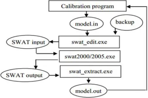
calibration/uncertainty analysis programs such as: SUFI2 (Abbaspour et al., 2007), GLUE (Beven and Binley, 1992), and ParaSol (Van Griensven and Meixner, 2006). The program allows the user to run the procedure several times until convergence is reached (Abbaspour et al., 2004). This study utilized a multi-site semi-automated inverse modeling routine SUFI-2 for calibration and uncertainty analysis for the Blunn Creek Watershed. The general concept how the SWAT-CUP works can be seen in the following figure (Figure 2-1) (Abbaspour et al., 2007).
Figure 2-1. Interaction between calibration program and SWAT in SWAT-CUP (Abbaspour, 2007).
21
SWAT-CUP program writes the model parameters in model.in. Then, swat_edit.exe edits the SWAT text files, inserting the new parameter values. After that, SWAT simulator is run. Finally, the swat_extract.exe program extracts the desired variables from the SWAT output files and writes them to model.out. The procedure continues as required by the calibration program (Abbaspour, 2007).
This study utilized a multi-site semi-automated inverse modeling routine SUFI-2 for calibration and uncertainty analysis for the Blunn Creek Watershed in Austin, TX.
Methodology
SWAT-CUP Setup
Three main steps were taken in order to run SWAT-CUP. First of all, observed historical data were downloaded from USGS website for calibration purposes. Second, input parameters were converted into sub-hourly format through SWAT. Finally, inputs were entered and the SWAT-CUP program was run.
Observed stream discharges at USGS Station 08157700, operated by City of Austin (COA) after the year 2001, were retrieved in 15 min format from USGS (USGS, 2014) for the period between 1998 and 1999 for calibration purposes between 2001 and 2002 for validation purposes. Flow data were modeled and compared to observed data for calibration purposes.
It should be noted at this point that SWAT-CUP version 5.1.4.2 that was used in this study is designed for daily, monthly and yearly time steps though it can read and accept hourly or sub-daily format because it calls data from the TXINOUT folder that is already exported from and formatted by SWAT. The following steps were followed to
22
convert the daily model to a sub-hourly time step model: 1) subdaily weather data for precipitation and temperature were used to do an initial run of SWAT; 2) the fig.fig file located in the TXINOUT folder in a SWAT project was changed by including a new saveconc command for sub-hourly output. This command saves flow, sediment and water quality data from a specified point to a file (Figure 2-2). The first input number of the command which appears in the red box in Figure 2 represents the command code (14). The second input (41) represents the hydrograph storage location number of the data to be printed to the file. The third number (2) is the unique sequential file number for the saveconc command and the fourth input number (1) represents the printing frequency and value of 1 represents the sub-hourly printing frequency. The default printing value (0) given by SWAT is for daily averages unless another printing frequency is input. The last row before the finish command is the name of file where data will be saved and printed (watout.dat) (Neitsch et al., 2005).
23 Calibration Parameters
The parameters responsible for stream-flow assessment for the Blunn creek watershed were defined in the SWAT-CUP program under the calibration input parameters tab and under the Par_inf.txt file (Table 1) in order to be optimized. Since SWAT is a distributed hydrological model, there are potentially many parameters that can affect the stream flow assessment. Investigating the potential impact of all these parameters can be a very difficult task due to the high number of parameters and the complex interaction between them. Furthermore, looking at a sub-hourly time step format would result in a more complex model since it accounts for more details than daily or monthly time step. Therefore, utilizing an automated model such as SWAT-CUP rather than manual calibration becomes very important to save time and achieve higher accuracy. An Initial run that accounts for all available parameters (Table 2-1) was conducted.
Table 2-1. Initial calibration parameters given by SWAT-CUP Parameter name Description
r__CN2.mgt Initial SCS runoff curve number for moisture condition II v__ALPHA_BF.gw Baseflow alpha factor (1/day)
v__GW_DELAY.gw Groundwater delay (days)
v__GWQMN.gw Threshold depth of water in the shallow aquifer required
for return flow to occur (mm)
v__GW_REVAP.gw Threshold depth of water in the shallow aquifer for
"revap" to occur
v__ESCO.hru Soil evaporation compensation factor v__CH_N2.rte Manning roughness for main channel v__CH_K2.rte Effective hydraulic conductivity v__ALPHA_BNK.rte Baseflow alpha factor for bank storage
r__SOL_AWC(1).sol Available water capacity of the soil layer (mm H2O/ mm
soil)
r__SOL_K(1).sol Saturated hydraulic conductivity (mm/hr) r__SOL_BD(1).sol Moist bulk density (g/cm3)
24
The duration of the simulation (beginning and ending) is defined under SUFI2_swEdit.def. The number of years to be simulated, beginning and end of the simulation, and the number of warm up periods are defined under the File.Cio file, which is a SWAT file. All the parameters to be fitted plus their minimum and maximum ranges are defined under Absolute_SWAT_Values.txt. Default values for the fitted
parameters and their ranges given by SWAT-CUP were used. Observed values that correspond to the variables in output.rch file were edited after converting it into sub-hourly format under observed_rch .txt. The name of variables to be extracted from the output.rch.txt files were defined under Var_file_rch_txt which is in this case only flow. Uncertainty Analysis
Five objective functions were selected to analyze model efficiency of stream flow calibration for the Blunn creek watershed; P-factor (ranges between 0% and 100%), R-factor (ranges between 0 and infinity), R2, NS and bR2 (which is the coefficient of determination multiplied by the coefficient of regression). The best-fit of the model can be quantified by the coefficient of determination (R2) and Nash–Sutcliffe efficiency (NS) between the observations and the final best simulations. Default values and ranges given by SWAT-CUP for other variables (soil, HRU, groundwater, basin, subbasin, .etc.) were selected. The objective function type was selected to be NS coefficient with 0.5
minimum value of objective function threshold for the behavioral solutions. The output of the initial run that can be found in the watout file within the TXINOUT folder was printed in 15 minutes time steps. The main outcome variable in SWAT-CUP was defined to be flow with 14 reaches/subbasins and to account for one reach in each
25
subbasin. The preprocessing procedures, which include running the Latin hypercube sampling program was executed followed by running SUFI-2_execute.exe program that runs the SWAT_Edit.exe extraction file as well as SWAT.exe. SUFI2_post.bat file in order to estimate objective function, 95 PPU calculation, 95 PPU for behavioral simulation and 95 for the variables with no observations. An integrated sensitivity analysis for all parameters utilized in the initial run was printed out in conjunction to calibration outputs. Only the most sensitive parameters based on t-statistic and p-value were selected for a second run of calibration.
Case Study
This case study is based on research conducted in Austin, Texas and specifically the Blunn Creek Watershed (Figure 2-3). The watershed was estimated to have 34.8% impervious cover in 2003 and the total catchment area is 1 square mile. The creek has a length of three miles. The total population estimated to be living in the watershed area
26
in 2013 is 6,000 and the projected to be 6810 by 2030 might (COAa, 2013).
Figure 2-3. Blunn Creek Watershed in Austin, Texas.
The selection of the SWAT model was mainly because it is an integrated model that accounts for most hydrological components is easily accessible, in the public domain, and much of the input data are readily available. Also, the integration of the model with GIS environment allows the user to utilize all GIS tools to modify, add and edit layers to SWAT maps. SWAT 2012.10.4 was used and modified to run on a sub-hourly time step. Models were run using 15 minute rainfall data from the Flood Early
27
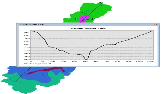
Warning System (FEWS) and Water Quality Monitoring (WQM) sections at COA, sub-hourly temperature data from the Austin and Austin-Bergstrom NOAA weather stations (WGEN_US_COOP_1960_2010), a 10-ft integer Digital Elevation Model (DEM) developed by COA based on 2003 LIDAR data and SSURGO soils data from NRCS. Geometry of the channels for each sub-basin was modified after conducting a cross-section analysis for the DEM layer. The cross-cross-section analysis was done by converting the DEM layer using an interpolation line tool under 3D Analyst menu in ArcGIS and creating a profile graph (Figure 2-4) and calculating the dimensions of an equivalent trapezoidal cross-section.
28
The specific objectives of the case study are to model the hydrology of the Blunn Creek Watershed using SWAT program and the calibration and validation of this model using SWAT-CUP.
Results
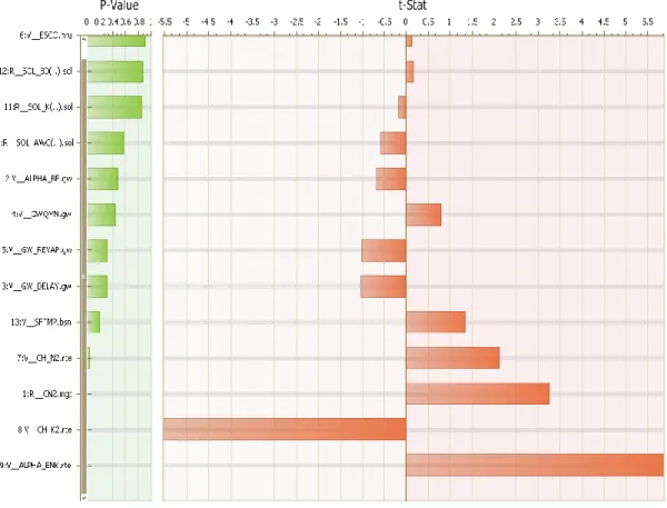
The results of a global sensitivity analysis of stream-flow parameters using Latin hypercube regression systems is shown in Figure 2-5. Eight parameters were selected for calibration based on the results of sensitivity analyses that varied all parameters
simultaneously, (Table 2-2).
Table 2-2. Stream flow parameters selected for calibration Stream flow parameters
selected for calibration*
Description
v__ALPHA_BF.gw Base flow alpha factor v__GW_DELAY.gw Groundwater delay
v__GWQMN.gw Threshold depth of water in the shallow aquifer required for return flow to occur
v__CH_N2.rte Manning roughness for main channel v__CH_K2.rte Effective hydraulic conductivity
r__SOL_AWC Available water capacity of the soil layer V_ESCO.hru Soil evaporation compensation factor r__SOL_K(1).sol Saturated hydraulic conductivity
* Description of each qualifier: “v” means that parameter value is replaced by a value from the given range and “r” means that parameter value is multiplied by (1 + a given value) (Abbaspour et al., 2007)
29
Figure 2-5. Global sensitivity analysis for an initial run that accounts for all uncertainty parameters
The parameters have given ranks for their sensitivity to the model calibration (Table 2-3).
30
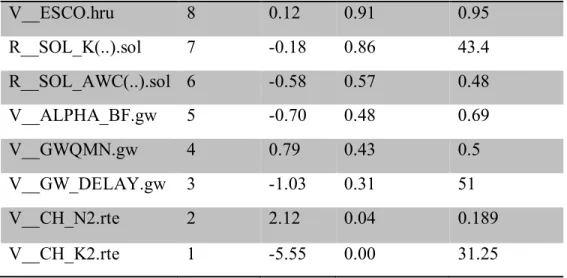
Table 2-3. Parameter sensitivities for SUFI-2
Parameter_Name Ranking t-stat P-value Si
V__ESCO.hru 8 0.12 0.91 0.95 R__SOL_K(..).sol 7 -0.18 0.86 43.4 R__SOL_AWC(..).sol 6 -0.58 0.57 0.48 V__ALPHA_BF.gw 5 -0.70 0.48 0.69 V__GWQMN.gw 4 0.79 0.43 0.5 V__GW_DELAY.gw 3 -1.03 0.31 51 V__CH_N2.rte 2 2.12 0.04 0.189 V__CH_K2.rte 1 -5.55 0.00 31.25
Table 2-4 below shows the minimum and maximum ranges of the parameters fitted for the sub-hourly calibration in the SUFI-2.
Table 2-4. Stream flow calibration parameter uncertainties Parameter Name Fitted
Value File name Minimum value Maximum value V__ALPHA_BF.gw 0.25 .gw 0 1 V__GW_DELAY.gw 350.25 .gw 30 450 V__GWQMN.gw 1.95 .gw 0 2 V__ESCO.hru 0.88 .hru 0.8 1 V__CH_N2.rte 0.23 .sub 0 0.3 V__CH_K2.rte 30.52 .sub 5 130 R__SOL_AWC(..).sol 0.0025 .sol -0.2 0.4 R__SOL_K(..).sol 0.31 .sol -0.8 0.8
The manning coefficient (Ch_N2) fitted value suggested by SWAT-CUP was far from expectation. One possible explanation that baseflow was not being well simulated in SWAT due to lack of input in precipitation during non-rainy days. This resulted in
31
water balance errors and that was compensated by SWAT-CUP by increasing the manning roughness coefficient. We expect that if analysis was made with manning coefficient = 0.035 only, baseflow would be affected then the results of this study should be valid for the calibration run produced by SWAT-CUP. The remaining default
uncertainty parameters given by SWAT-CUP were tested as a double check test and they had no significant effect on stream-flow simulations. Updating the values of the
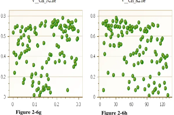
remaining parameters did not result in significant changes in the model output. The distribution of the number of simulations in the parameter sensitivity analysis was plotted after comparing the parameter values with the objective functions for the sub-hourly calibrations (Figure 2-6). The x-axis in this figure is the paramter value and the y-axis is the objective function value (NS).
Figure 2-6 Sensitive parameters during sub-hourly calibration for the Blunn Creek Watershed vs. objective function. a: Threshold depth of water in the shallow
aquifer required for return flow to occur, b: Soil evaporation compensation factor, c:Available water capacity of the soil layer, d: Saturated hydraulic conductivity, e: Groundwater delay, f: Base flow alpha factor, g: Manning roughness for main channel, h: Effective hydraulic conductivity
32
Figure 2-6f Figure 2-6e
Figure 2-6c Figure 2-6d
33
Results from SUFI-2, for the sub-hourly calibration showed that the alpha base flow factor (Alpha_BF), the soil evaporation compensation factor (ESCO), the threshold depth of water in the shallow aquifer required for return flow to occur factor (GWQMN) and the ground water delay factor (GW_DELAY) had a wide range in their values (Figure 2-6a,b,e), whereas, the soil effective hydraulic conductivity and Manning
roughness for the main channel show large variation in their values (Figure 2-6 h,g). The goodness-of-fit and efficiency of the model were tested using the main objective
functions listed above. These five objective functions were analyzed on a sub-hourly basis correspondingly for SUFI-2 uncertainty technique (Table 2-5) for the best-fit model
Figure 2-6g Figure 2-6h
34
Table 2-5. Stream flow calibration results for sub-hourly model
Variable Value p-factor 56% r-factor 0.54 R2 0.78 NS 0.78 b R2 0.6423 MSE 0.0035 SSQR 0.0005
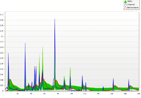
After observing model performance and running initial iterations using SWAT-CUP with all input parameters to be optimized (Figure 2-7) , the baseflow was
systematically overestimated at the outlet of the watershed (in subbasin 1), and there is a late shift in the flow peak.
35
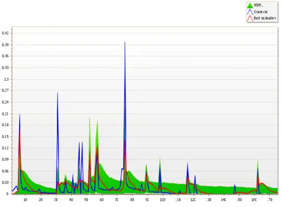
The following steps were taken to fix this problem; baseflow factor was decreased, deep percolation (GWQMN) was increased, the groundwater revap
coefficient (GW_REVAP) was increased, and the threshold depth of water in shallow aquifer (REVAPMN) was decreased. To correct the peak flow delay, the slope
(HRU_SLP) was increased, Manning’s roughness coefficient (OV_N) was decreased, the value of overland flow rate (SLSUBBSN) was decreased, and snow melt parameters (SMTMP) were decrease. Figure 2-8 shows the result after applying these steps as well as considering only the eight parameters included in the calibration (Table 2-2). Clearly, adjusting the previous parameters resulted in simulated data that match the observed data better with respect to peak flow and time to peak.
36
The water balance of the model results for the calibration periods was performed in order to assess the validity of the calibrated and validated model (Table 2-6). The inflow of the water balance (Eq. 4) is precipitation and the return flow originated by groundwater as it is descried in SWAT 2012 manual. The outflow/losses are represented by surface runoff, evapotranspiration and percolation. It should be noted that irrigation application was applied with a frequency of nine applications for each HRU and with a total volume of 227.84 mm as SWAT output file showed for the 24 simulation period. The following land uses were excluded from irrigation application: parks, undeveloped lands, open spaces, transportation and infrastructure, and camp ground. The error percentage was calculated by dividing losses by inflow.
Table 2-6. Average annual water balance components and error percentages for the calibration period at the Blunn Creek Watershed
Component Calibration/Depth (mm)
(1998 and 1999) Validation/ Depth (mm)
(2001 and 2002)
Precipitation 1484.1 1878
Surface Runoff 466.29 575
Lateral Flow contribution to
stream flow 73.06 96.69
Groundwater contribution
to stream flow 3.28 6.91
Water percolation 32.94 72.79
Drainage Tile 0 0
Amount of water stored in
soil 192.83 315.41
Actual ET 1262.17 1406.36
37
The validation period was the years 2001 and 2002.. NS value for validation was 0.67 and R2 value equals to 0.70 for sub-hourly time step model. It should be noted that both calibration and validation procedures were run for the entire two year period in addition to another two year warming up period. These results show that SWAT-CUP can be used to calibrate and validate SWAT when used for sub-hourly time steps. Accordingly SWAT can be used to estimate peak flow times during a storm and can be used for applications that occur at a sub-hourly scale such as low impact development hydrology.
Conclusions
Sub-hourly simulation model has been optimized successfully using SWAT 2012 and calibrating using SWAT-CUP, SUFI2 procedures. SWAT-CUP presented an
effective graphical interface in order to visualize calibration components such as observed data, simulated data, 95 PPU and the best fit model. The sensitivity analysis adopted for stream flow calibration was very successful and contributed to optimizing the total number of uncertainty parameters and accordingly more efficient calibration procedures. SUFI-2 gave good results in minimizing the differences between simulated and observed data for the sub-hourly time step model. The P-factor and R-factor calculated using SUFI-2 procedures have provided good agreement by bracketing around 54- 56% observed data on a sub-hourly basis. Results showed acceptable matching between simulated and observed flows for the Blunn Creek Watershed for the simulation period. The presented study showed that the sub-hourly SWAT model results in a reasonable stream flow hydrograph under multiple storm events. Calibrated stream
38
flows for a 2 year period with 15- min simulation had (R2= 0.78) and (NS =0.78). Validation procedures for a 2 year period showed acceptable correlation between simulated and observed data, NS value is 0.67 and R2 value equals to 0.70. This study showed how a sub-hourly model can be run using SWAT and calibrated using SWAT- CUP for a long simulation period. Calibrating and validating a sub-hourly model for a long duration instead of single storm was attained. The ability to optimize the best set of parameters to minimize the uncertainty for a complex system is an important tool with a complex watershed model, enhancing the ability to select the “best” model from a multitude of models with varying parameter sets which may provide similar results.
39
CHAPTER III
MODELING STREAM BANK EROSION AT A WATERSHED SCALE IN
THE BLACKLAND PRAIRIE ECOSYSTEM
Synopsis
Stream bank erosion is a naturally occurring process that includes the removal of soil particles due to change in stream flow, and the discharge of runoff from other sources. The goal of this study was to investigate the capability and performance of sub-hourly time steps SWAT models in predicting of stream flow in the Blackland Prairie ecosystem and to estimate potential stream bank erosion. The major steps carried out to achieve this objective include; sensitivity analysis for sub-hourly time step SWAT models, development of two methodologies to represent bioretention and permeable pavement into SWAT, analysis of shear stress and excess shear stress for stream flows under different development scenarios and in conjunction with different levels of LID practices, and estimating potential stream bank erosion for different median soil particle sizes using real and design storms.
A sub-hourly SWAT model was successfully calibrated and validated for stream flows. Calibrated stream flows for a 2-year period using the 15-minute time step had an R2 of 0.78 and an NS of 0.78. The 2 year validation period had an R2 of 0.70 and a Nash Sutcliffe (NS) of 0.67. Results showed that combining permeable pavement and
bioretention area resulted with the greatest reduction percentages in runoff volumes, peak flows, and excess shear stress under both real and design storms. Adding bioretention only resulted with the second greatest reduction percentage and adding
40
detention pond only had the least reduction percentages. Results showed agreement between modeling data and field experiments’ findings. The soil particle with median diameter equals to 64 mm had the least excess shear stress among all design storms, while 0.5 mm soil particle size had the largest magnitude of excess shear stress. The larger the value of excess shear stresses, the higher the potential of erosion to happen.
Introduction
Changing land due to urbanization increases the amount of stormwater runoff which in turn can have harmful effects on urban and suburban streams, both
hydrologically and biologically. As streams meander across the surface of the earth, they erode their beds and banks in a dynamic natural way (Staley et al., 2006). Several research studies have demonstrated the significant contribution of stream bank erosion to total sediment loading (Simon and Darby, 1999; Sekely et al., 2002; Evans et al., 2006). Konrad et al., (2005) studied the impact of urban development on stream flow and stream bed stability. They examined 16 streams in the Puget Lowland, Washington, using three stream flow metrics that integrate storm-scale effects of urban development over annual to decadal timescales. They concluded that the increase in the magnitude of frequent high flows due to urban development but not their cumulative duration has important consequences on channel form and bed stability in gravel bed streams.
In order to restore or maintain channel stability, the incision of the channel bed and erosion of the stream banks must be prevented. Stability of a streambed can be attained by acquiring the balance between sediment supply and sediment transport capacity, while stream bank stability can be attained by maintaining the applied shear
41
stress to be below erosive thresholds (Lawler, 1995). These thresholds can be estimated by defining the critical shear stress at which soil detachment begins. The erosion rate will remain zero as long as the critical shear stresses are higher than the applied shear stress (Hanson et al., 2002; Nearinget al., 1989). Sediments resulting from stream bank erosion can account for 85% of watershed sediment yields and bank retreat rates of 1.5 to 1100 m/year have been documented in several studies (Prosser et al., 2000; Simon et al., 2000; Wallbrink et al., 1998) .The total damage to natural resources and human health due to water pollution by sediment costs an estimated $16 billion annually in North America (Osterkamp et al., 1998).
Erosion control and management of urban streams is becoming increasingly important because of the economic damage that stream bank erosion can cause along urban streams and impairment of water quality. Low Impact Development (LID) was developed to mimic the natural water cycle of the land by reducing the negative impact of stormwater runoff on water bodies and eventually human health. LID practices are structural or non-structural management practices that aim to decrease the impacts of urbanization and sediments on water quality. LIDs include the installation of any of the following structural measures to retrofit existing infrastructure and reduce runoff volumes and peak flows: bioretention, green roofs, rainwater harvesting, and permeable pavements (Damodaram, 2010). Regulatory enforcement of LID implementation results in an urgent need for quantitative information on LID effectiveness for sediment and stream erosion (Lee and Jones-Lee, 2002). While LID practices have been mentioned in literature for stormwater management (Dietz and Clausen, 2008; Elliott and Trowsdale,
42
2007; Hood et al., 2007; Bedan et al., 2009) there is little research that studied LID practice impact with respect to reducing stream bank erosion in urban areas.
Jeong et al. (2011) developed a sub-daily algorithm which was integrated into SWAT to simulate LIDs such as detention basins, wet ponds, sedimentation filtration ponds, and retention irrigation systems. The algorithm was tested for predicting sediment yield and total runoff but not for potential stream bank erosion. Krishnappan and Marsalek (2002) conducted an experiment in a rotating circular flume to test for transport characteristics of sediment from an on-stream stormwater pond in Kingston, Ont., Canada. The main findings of this experiment were that the sediments from the pond exhibited cohesive behavior and formed particle aggregates when subjected to a flow field. The experiment provided data on the sediment fraction which would deposit under specific shear stress and the deposited sediment fraction which would be eroded. Bledsoe (2002) designed a detention pond based on time-integrated sediment-transport capacity. They examined the impact of the detention pond in reducing stream channel erosion for two bed material sizes (8mm and 0.5 mm). They concluded that the followed methodology of design resulted in channel instability and substrate changes and they recommended developers to account for the frequency distribution of sub-bankfull flows, the capacity to transport heterogeneous bed and bank materials, and potential shifts in inflowing sediment loads before conducting a design. Furthermore, other studies addressed LID practices
effectiveness through field experiments, but not through computer simulations that are capable of covering wider scales. Field experiments are costly and difficult to duplicate, though computer simulation can be run several times with a numerous number of

![Figure 3-5. Schematic of Austin sedimentation/filtration basins [Courtesy of City of Austin (2011)]: (a) configuration of full/partial sedimentation filtration basins; (b) riser pipe outlet system and flow spreader in full type systems](https://thumb-us.123doks.com/thumbv2/123dok_us/1986724.2795063/70.918.201.646.629.972/schematic-sedimentation-filtration-courtesy-configuration-sedimentation-filtration-spreader.webp)