Probing the diffuse interstellar medium with diffuse interstellar bands

(1)

This work is protected by copyright and other intellectual property rights and duplication or sale of all or part is not permitted, except that material may be duplicated by you for research, private study, criticism/review or educational

purposes. Electronic or print copies are for your own personal, non-commercial use and shall not be passed to any other individual. No quotation

may be published without proper acknowledgement. For any other use, or to quote extensively from the work, permission must be obtained from the

(2)

medium with diffuse interstellar

bands

Amanda Bailey

Doctor of Philosophy

Environment, Physical Sciences and Applied Mathematics Research Institute, University of Keele.

(3)

Abstract

This work investgates the small scale structure of the Diffuse Interstellar Medium. To do this optical spectroscopy is used to obtain spectra of early type stars which are used as background targets with which the Diffuse Interstellar Medium (ISM) is probed. The spectra obtained contain the highly diagnostic Diffuse Interstellar Bands (DIBs), Na i _{D and Ca} ii _lines.

The maps I present here are of the Local Bubble, the Small Magellanic Cloud and the Large Magellanic Cloud. These are the ﬁrst DIB maps of the solar neighbour-hood and large portions of external galaxies. The specta were obtained with the New Technology Telecsope (NTT) at La Silla Observatory in Chile (Local Bubble survey) and at the Anglo-Australian Telescope (AAT) at Siding Spring Observatory, NSW, Australia. The NTT spectra are long slit spectra of 239 individual targets, whilst the AAT spectra were obtained with the multi-ﬁbre spectrograph 2dF/AAOmega (about 350 targets in each of the Magellanic Clouds).

I have succesfully used the 5780 and 5797 ˚A DIBs to map the ISM in the Local Bubble and the Magellanic Clouds. The 5797 ˚A DIB traced neutral structures whereas the 5780 ˚A DIB traced warmer and/or more highly irradiated gas, possibly residing in the skins of those neutral clouds It showed a more highly structured Local Bubble than revealed by the sodium maps, on sub parsec scales; tracing the walls of the Bubble and clearly showing the Bubble opening out into the Halo. In the Magellanic Clouds the DIBs trace molecular clouds surrounding regions of active star formation; they are weak or absent in quiescent molecular cloud complexes and hot gas bubbles.

(4)

Acknowledgements

“It is never too late to be what you might have been” – George Eliot

I dedicate this thesis to my late parents, Chris and Len Brown.

Dad did not know that I had returned to study; he never knew that our discussions about the Moon landings and my subsequent fascination with the stars would one day see me make a journey from observing high up in the mountain tops of Chile across to the other side of the world to China to attend a conference. I owe my insatiable curiosity and determination to our in-depth and often argumentative discussions. Mum did know that I had obtained a degree and had started my PhD, she knew I had travelled to observe and loved to hear about it all. She too was fascinated with astronomy and found a renewed interest as a result of my work. Although one of my observing trips to Australia was tinged with sadness at her passing while I was away, I do have a wonderful memory of her waving me off on that trip, a memory that got me through the most difficult parts of the PhD. I promised her I would complete it and I have. There are many other thanks to give for the support I have received while doing this PhD: the rest of my family, my son Josh, Sue and Rod in particular, for their support and encouragement; my supervisor, Jacco, for giving me the opportunity (and putting up with me!); Emily, for warning me what a nightmare it would be but also for just being there for me throughout; the “12:30 at Foyles” gang - Jon, Colin, Rob and Adam, with whom many a boozy lunchtime was spent discussing my work, life the Universe and everything; Donovan, Tony and the lads at the garage for achieving the impossible on more than one occasion and keeping my car on the road so I could get to Keele; the many friends and colleagues too numerous to mention from the Society for Popular Astronomy, the Open University, the Royal Astronomical Society and last but not least the Shropshire Astronomical Society. My final thanks go to Vic Tyne, as one of my Open University tutors and then a colleague at Keele, Vic bridged the two types of my study. Indeed, I really could not have done this without his encouragement.

(5)

List of Figures

1.1 Impression of the Local Bubble by C. Wellmann showing the location of

the Sun, (Frisch 1998). . . 6

1.2 Two spectra of the binary HD 23180 showing the Doppler shifts of the stellar lines and stationary nature of the interstellar features: Na, Si iii_{, known DIBs and claimed DIB detections marked with arrows,} (Kre lowski & Sneden 1993). . . 10

1.3 Composite DIB spectrum of DIBs listed in the 1994 DIB catalogue, (Jenniskens & Desert 1994). . . 12

1.4 Showing the relationship between the strong 5780 ˚A DIB and E(B ₋V) 14 1.5 Origin of absorption and emmission lines . . . 22

2.1 The polynomial ﬁt (top trace) used to normalise the ﬂat frame (bottom trace) is not appropriate. This is shown for one row of the frame. . . . 35

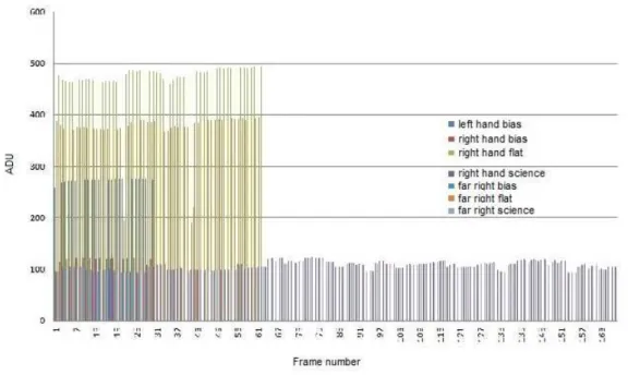
2.2 Bar chart showing the median values of the bias, ﬂat and science frames from the 22nd March 2011. . . 37

2.3 Bar chart showing the median values of the bias frames from the 20th August 2012. . . 39

2.4 Dispersion relation for 19th August 2012. . . 43

2.5 Identiﬁcation of telluric lines in the 6290 ˚A region . . . 44

2.6 Potential targets chosen for the SMC and LMC . . . 51

2.7 The conﬁgure mimic window once the allocation process has been com-pleted and the ﬁbre positions drawn . . . 53

2.8 Typical result from the Plot Tram Map option after zooming in . . . . 55

2.9 Correct appearance of a reduced arc exposure . . . 55

2.10 Illustrating the relationship between equivalent width and the area of an absorption line. (credit: Arizona.edu, Lecture 15: Stellar Atmospheres, Variable Stars). . . 66

3.1 Plot of 3-D spatial distribution of interstellar Na i _{absorption in the} Local Bubble . . . 88

3.2 Locations of the observed target stars in RA and Dec. Distance is rep-resented by the size of the symbol as given in the legend. . . 90

3.3 The average proﬁle of the 5780 ˚A DIB showing the blended stellar feature at 5785 ˚A successfully removed from the DIB proﬁle and also showing the much weaker 5797 ˚A DIB. . . 93

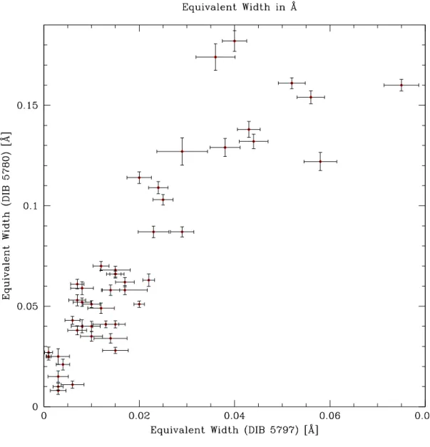
3.4 The average profiles of the 5850, 6196, 6203, 6270, 6283 and 6614 ˚A DIBs and the average profiles of the He and Na D lines. . . 94 3.5 Correlation between the equivalent widths of the 5780 and 5797 ˚A DIBs. 95 3.6 Profiles of the 5780 and 5797 ˚A DIBs, showing that there are

(9)

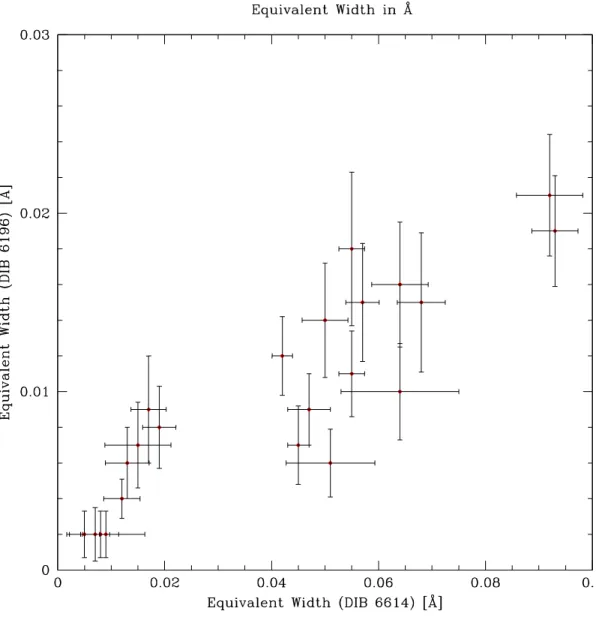
3.7 Correlation between the equivalent widths of the 6196 and 6614 ˚A DIBs. 99 3.8 Proﬁles of the 6196 and 6614 ˚A DIBs showing the reduction in DIB

strength with target star location . . . 100 3.9 Spectra of HD186500 and HD179406 showing that the 6614 ˚A DIB may

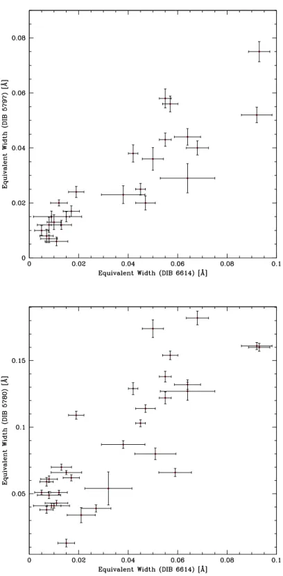
correlate well with the 5797 ˚A DIB. . . 102 3.10 Correlation between the equivalent widths of the (Top:) 5797 and 6614 ˚A

DIBs and (Bottom:) 5780 and 6614 ˚A DIBs. . . 103 3.11 Correlation between the equivalent widths of the (Top:) 5797 and 6196 ˚A

DIBs and (Bottom:) 5780 and 6196 ˚A DIBs. . . 104 3.12 Correlation between the equivalent widths of the (Top:) 5780 ˚A DIB and

the Na D2 line and (Bottom:) 5797 ˚A DIBs and the Na D2 line. . . 106

3.13 Profiles of the Na D lines showing the typical different profiles of the overlying broad absorption feature (blue) and the fitted Na D line profiles (red). . . 108 3.14 Identification of telluric lines in the 5930 ˚A region . . . 109 3.15 Plots of the Galactic latitude v EW for (Top:) the 5780 ˚A DIB, (Middle:)

the 5797 ˚A DIB and (Bottom:) the Na D2 line. . . 115

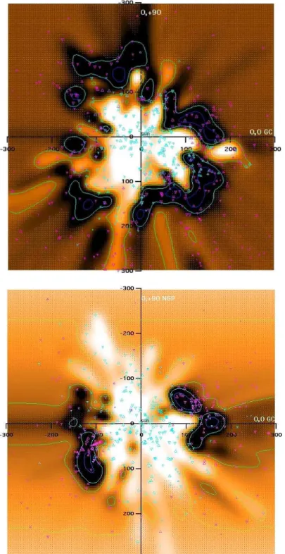
3.16 EW maps in Galactic coordinates of (Top Left:) the 5780 ˚A DIB ab-sorption, (Top right:) the 5797 ˚A DIB absorption and (Bottom:) the Na i _D₂ _{absorption. . . 117} 3.17 EW maps in the Galactic Plane projection of (Top:) the 5780 ˚A DIB

absorption and (Bottom:) the same map including all the sight lines for which there was no 5780 ˚A DIB absorption detected (marked in blue). . 120 3.18 EW maps in the Galactic Plane projection of (Top:) the 5797 ˚A DIB

absorption and (Bottom:) the same map including all the sight lines for which there was no 5797 ˚A DIB absorption detected (marked in blue). . 123 3.19 EW maps in the Galactic Plane projection of (Top:) the Na i _D₂

ab-sorption and (Bottom:) the same map including all the sight lines for which there was no Na i _D₂ _{absorption detected (marked in blue). . . . 125} 3.20 EW maps in the Meridian Plane projection of (Top:) the 5780 ˚A DIB

absorption and (Bottom:) the same map including all the sight lines for which there was no 5780 ˚A DIB absorption detected (marked in blue). . 126 3.21 EW maps in the Meridian Plane projection of (Top:) the 5797 ˚A DIB

absorption and (Bottom:) the same map including all the sight lines for which there was no the 5797 ˚A DIB absorption detected (marked in blue).128 3.22 EW maps in the Meridian Plane projection of (Top:) the Na i _D₂

ab-sorption and (Bottom:) the same map including all the sight lines for which there was no Na i _D₂ _{absorption detected (marked in blue). . . . 130} 3.23 Maps of the 5780/5797 ˚A DIB ratio in (Top:) the Galactic Plane

(10)

4.1 Comparison of DIBs observed in the lines-of-sight towards Sk-70 120 and Sk-69 223 in the LMC and DIBs in two Galactic lines of sight (Cox et al. 2006) . . . 134 4.2 Distribution of targets in the SMC and LMC. . . 136 4.3 Average proﬁles of (Top:) the Ca ii _{K line, (Second:) the 5780 ˚}_{A DIB,}

(Third:) the 5797 ˚A DIB and (Bottom:) the Na i _{D lines in the SMC.} ₁₃₉ 4.4 Average proﬁles of (Top:) the Ca ii _{K line, (Second:) the 5780 ˚}_{A DIB,}

(Third:) the 5797 ˚A DIB and (Bottom:) the Na i _{D lines in the LMC.} ₁₄₀ 4.5 Correlation between the equivalent widths of the 5780 and 5797 ˚A DIBs

for the SMC component in the SMC sight-line. . . 143 4.6 Proﬁle of (Top:) target 479 which has a strong 5780 ˚A DIB

absorp-tion but little, if any, 5797 ˚A DIB and (Bottom:) target 135 which has very strong Na absorption and also shows strong 5780 and 5797 ˚A DIB absorption. . . 144 4.7 Correlation between the equivalent widths of the 5780 and 5797 ˚A DIBs

for the Galactic component in the SMC sight-line, (Top:) all targets, (Bottom:) cropped version. . . 145 4.8 Proﬁle of target 215 showing the anomaly around the 5797 ˚A DIB in the

SMC. . . 146 4.9 Correlation between the equivalent widths of the 5780 and 5797 ˚A DIBs

for the LMC component in the LMC sight-line. . . 147 4.10 Correlation between the equivalent widths of the 5780 and 5797 ˚A DIBs

for the Galactic component in the LMC sight-line. . . 148 4.11 Proﬁle of target 1491 showing the the unreliability of the 5797 ˚A DIB. . 149 4.12 Correlation between the equivalent widths of the 5780 ˚A DIB and Na i

D2 line for (Top:) the SMC and (Bottom:) the LMC. . . 151

4.13 Correlation between the equivalent widths of the 5780 ˚A DIB and Na i D2 line for the Galactic component in (Top:) the SMC sight-line and

(Bottom:) the LMC sight-line. . . 153 4.14 Correlation between the equivalent widths of the 5797 ˚A DIB and Na i

D2 line for (Top:) the SMC and (Bottom:) the LMC. . . 155

4.15 Correlation between the equivalent widths of the 5797 ˚A DIB and Na i D2 line for the Galactic component in (Top:) the SMC sight-line and

(Bottom:) the LMC sight-line. . . 156 4.16 Correlation between the equivalent widths of the 5780 ˚A DIB and Caii

K line in the SMC for the (Top:) the blue component and (Bottom:) the red component. . . 158 4.17 Correlation between the equivalent widths of the 5780 ˚A DIB and Caii

K line in the LMC for the (Top:) the blue component and (Bottom:) the red component. . . 159

(11)

4.18 Correlation between the equivalent widths of the 5780 ˚A DIB and Caii K line for the Galactic component along the SMC sight-line. . . 161 4.19 Correlation between the equivalent widths of the 5780 ˚A DIB and Caii

K line for the Galactic component for (Top:) the blue component and (Bottom:) the red component along the LMC sight-line. . . 162 4.20 Correlation between the equivalent widths of the 5797 ˚A DIB and Caii

K line in the SMC for the (Top:) the blue component and (Bottom:) the red component. . . 163 4.21 Correlation between the equivalent widths of the 5797 ˚A DIB and Caii

K line in the LMC for the (Top:) the blue component and (Bottom:) the red component. . . 164 4.22 Correlation between the equivalent widths of the 5797 ˚A DIB and Caii

K line for the Galactic component in the SMC sight-line. . . 166 4.23 Correlation between the equivalent widths of the 5797 ˚A DIB and Caii

K line for the Galactic component for (Top:) the blue component and (Bottom:) the red component along the LMC sight-line. . . 167 4.24 Equivalent width maps of (Left:) the Ca ii _{K line for the blueward}

absorption line, and (Right:) the redward absorption line in the SMC. The rectangle represents the SMC bar and the circle represents an area containing giant molecular clouds and is a star forming region. . . 172 4.25 Proﬁles of the Ca ii _{K line showing the double feature in the SMC}

component for (Left:) target 317 and (Right:) target 395. . . 173 4.26 Equivalent width maps of (Top left:) the Na i _D₂ _{absorption line, (Top}

right:) the Na i _D₁ _{absorption line and (Bottom:) the sum of the} ab-sorption lines in the SMC. The rectangle represents the SMC bar and the circle represents an area containing giant molecular clouds and is a star forming region. . . 174 4.27 Equivalent width maps of (Top left:) the 5780 ˚A DIB absorption line,

(Top right:) the 5797 ˚A DIB line and (Bottom:) the ratio of the 5780/5797 ˚A DIBs in the SMC. The rectangle represents the SMC bar and the cir-cle represents an area containing giant molecular clouds and is a star forming region. . . 176 4.28 Proﬁles of the 5780 and 5797 ˚A DIBs showing (Top:) a good detection

if target 356 and (Bottom:) a bad and unreliable detection in target 864. 177 4.29 Equivalent width maps of (Left:) the Ca ii _{K line absorption for the}

blueward absorption line, and (Right:) the redward absorption line in the LMC. . . 179 4.30 Proﬁles of the Ca ii _{K line showing the double feature in the LMC}

component for (Left:) target 1161 showing a blueward wing and (Right:) target 1132 showing a redward wing. . . 180

(12)

4.31 Proﬁles of the Na i _D₁ _{and D}₂ _{absorption lines. Showing (Top:) an} example of good separation between the Galactic Nai_D₁ _{and the LMC} Na i _D₂ _{lines, (Middle:) a typical blended proﬁle showing evidence of} the two components and (Bottom:) an example where the fact there are two components is barely noticeable. . . 182 4.32 Equivalent width maps of (Top left:) the Na i _D₂ _{absorption line, (Top}

right:) the Na i _D₁ _{absorption line and (Bottom:) the sum of the} ab-sorption lines in the LMC. . . 183 4.33 Proﬁles of the Na i _D₁ _{and D}₂ _{absorption lines. Showing (Top:) an}

uncertain detection the the LMC bar region, (Middle:) a positive but weak detection to the North of the LMC bar and (Bottom:) a negative detection to the North of the LMC bar. . . 184 4.34 Equivalent width maps of (Top left:) the 5780 ˚A DIB absorption line,

(Top right:) the 5797 ˚A DIB line and (Bottom:) the ratio of the 5780/5797 ˚A DIBs in the LMC . . . 186 4.35 Proﬁles of the 5780 and 5797 ˚A DIBs showing (Top:) a good detection

and (Bottom:) a bad and unreliable detection. . . 187 4.36 Equivalent width map of the Ca ii _{K line in the Milky Way Galaxy in}

the direction of the SMC. . . 189 4.37 Proﬁle of the Ca ii _{K line showing a very broad feature in the Galactic}

component. . . 190 4.38 Equivalent width maps of (Top left:) the Na i _D₂ _{absorption line, (Top}

right:) the Na i _D₁ _{absorption line and (Bottom:) the sum of the} ab-sorption lines in the Milky Way Galaxy in the direction of the SMC. . 191 4.39 Proﬁles of the Na i _D₁ _{and D}₂ _{lines showing (Top:) the D}₁ _{and D}₂

components in both the Galactic component and the SMC component and (target 21) (Bottom:) an example where the Na is present in the Galactic observations but absent in the SMC observations (target 104). 192 4.40 Equivalent width maps of (Top left:) the 5780 ˚A DIB absorption line,

(Top right:) the 5797 ˚A DIB line and (Bottom:) the ratio of the 5780/5797 ˚A DIBs in the Milky Way Galaxy in the direction of the SMC. . . 194 4.41 Proﬁles of the 5780 ˚A and 5797 ˚A DIBs showing that the 5780 ˚A DIB is

the stronger of the two in the Galactic region (target number 867). . . 195 4.42 Proﬁles of (Left:) the 5780 ˚A DIB (target number 182) and (Right:) the

5797 ˚A DIB (target number 702) showing that these DIBs are weaker in the Galactic region than they are in the SMC. . . 196 4.43 Equivalent width maps of (Left:) the Ca ii _{K line absorption for the}

blueward absorption line, and (Right:) the redward absorption line in the Milky Way Galaxy in the direction of the LMC. . . 197

(13)

4.44 Proﬁles of (Top:) similar strength blueward and redward components (target number 1116), (Middle:) a stronger blueward component (target number 1121) and (Bottom:) a stronger redward component (target number 967) of the Ca ii _{K line . . . 198} 4.45 Equivalent width maps of (Top left:) the Na i _D₂ _{absorption line, (Top}

right:) the Na i _D₁ _{absorption line and (Bottom:) the sum of the} ab-sorption lines in the Milky Way Galaxy in the direction of the LMC. . 200 4.46 Proﬁles of (Left:) stronger Na absorption in the LMC component (target

number 1831) and (Right:) no Na absorption in the LMC component (target number 826). . . 201 4.47 Equivalent width maps of (Top left:) the 5780 ˚A DIB absorption line,

(Top right:) the 5797 ˚A DIB line and (Bottom:) the ratio of the 5780/5797 ˚A DIBs in the Milky Way Galaxy in the direction of the LMC. . . 203 4.48 Proﬁles of (Left:) weaker 5780 ˚A DIB in Galactic component and (Right:)

weaker 5797 ˚A DIB in Galactic component (target number 1262 for both). . . 204 5.1 A schematic diagram of a σ type or ’skin-eﬀect cloud. With thanks to

(14)

List of Tables

2.1 Characteristics of the CCD used at the NTT . . . 26

2.2 Parameters used on 2dfdr to reduce the data. . . 57

2.3 Constraints for ﬁtting absorption lines . . . 64

2.4 Constraints for ﬁtting absorption lines. . . 79

3.1 Values of the correlation calculations between the 5780 and 5797 ˚A, and the 6196 and 6614 ˚A DIBs; also showing the t-test values and the corre-sponding critical values oft. . . 112

3.2 Values of the correlation calculations between the 5797 and 6614 ˚A, 5780 and 6614 ˚A, 5797 and 6196 ˚A and also 5780 and 6196 ˚A DIBs; also show-ing thet-test values and the corresponding critical values of t. . . 113

4.1 Values of the correlation coeﬃcients between the 5780 and 5797 ˚A DIBs for the SMC data; also showing the t-test values and the corresponding critical values of t. . . 169

4.2 Values of the correlation calculations between the 5780 and 5797 ˚A DIBs for the LMC data; also showing the t-test values and the corresponding critical values of t. . . 169

(15)

1 Introduction and literature review

“Astronomy compels the soul to look upwards and leads us from this world to another”

- Plato

1.1 Motivation

The Interstellar Medium (ISM) is both the birthplace of stars and their ﬁnal resting place; the alpha and the omega. As such it is an incredibly complex and diverse environment the study of which is paramount to our understanding the evolution not only of stars, planets and galaxies but ultimately of life itself. In fact, the study of galaxy evolution would not be complete without accounting for the Interstellar Medium. Galaxies are ecosystems in which stars form, evolve and die; constantly interacting with the ISM.

Surprisingly, small, neutral ISM structures are encountered in both the cold ISM and in the much warmer (weakly-)ionized diffuse ISM. This poses many questions one of which is “Are the materials that make up these small structures the same or different in each type of environment?” By using Diffuse Interstellar Bands (DIBs), some of which are known to form in hot, UV-irradiated environments while others form in cooler environments, we can probe the distribution of material and conditions within extreme environments such as the Local Bubble (LB) and the Disc-halo interface. Thus, we can learn about the nature of the diffuse Interstellar Medium in such regions.

1.2 The Interstellar Medium

The Interstellar Medium consists of a tenuous gas of hydrogen and helium enriched with a scattering of heavier elements. Whether the gas of the ISM occurs as ions, molecules

(16)

or atoms depends upon the presence of radiation ﬁelds as well as the temperature and density of the gas.

The ISM is a turbulent and dynamic place where the majority of its volume con-tains diﬀuse (n _∼0.1 cm−3

) hot ionised gas (T _∼105

K) in which most of the gas mass is either in HI clouds (102

K < T < 104

K) or in cold, dense, star forming molecular clouds (T < 102

K), (Avila-Reese 2007; Cox 2005). In small scale interactions stars re-turn chemically enriched gas to the ISM by ionising radiation and stellar winds. Large scale interactions such as supernovae return the enriched gas to the Galactic Halo or inter-galactic space where it cools and rains down onto the Galaxy or is accreted by another galaxy close by (Bland-Hawthorn et al. 2007). The molecular clouds in which star formation occurs appear to form during the large scale compression of the ISM by supernova explosions (Avila-Reese 2007), colliding gas flows or spiral wave gravi-tational modulations. The intense star formation also produces massive gas outflows in the form of galactic fountains and winds returning material into galactic and inter-galactic space. The ISM on small scales often displays filamentary structure resulting from hydrodynamic and thermal dynamic instabilities in environments ranging from supernova remnants to the diffuse interstellar cirrus.

1.3 The Local Bubble

The Local Bubble is a desolate place, it is a cavity in the interstellar medium that con-tains so little matter it can be considered a near-perfect vacuum. Nevertheless our solar system is embedded within this desolate region. This gives us the unique opportunity to study the interstellar gas in such extreme environments via accurate absorption line measurements along lines-of-sight which are essentially free from intervening contam-inating features. The LB is a region of unusually low gas density in the interstellar medium (ISM); it extends for _∼ 100 pc in the plane of the Galaxy and for hundreds of parsecs vertically, presumably as far as the galactic halo (Welsh et al. 1999; Welsh et al. 2010).

(17)

Conditions in the ISM can be probed in many ways; for example: Ovi_absorption, absorption lines arising from neutral or singly-ionized atoms or molecules, X-ray and synchrotron emission. However, there is a problem with understanding the nature of the gas within the LB using the absorption line method as such atoms and molecules are not expected to survive at the high temperatures inferred for the LB. To overcome this problem it is necessary to probe the LB using species which may survive under these conditions. To achieve this we use absorption in the Diﬀuse Interstellar Bands. The carriers of DIBs are thought to be large molecules such as polycyclic aromatic hydrocarbons and such molecules are resistant to UV radiation.

The DIBs are a set of over 400 broad optical absorption features which are om-nipresent in the ISM; for reviews see Herbig (1995), Sarre (2006). They are absorption bands in the visual and near-infrared spectral region. Their carriers are, as yet, un-known but are likely to be molecular. I will describe them in more detail in section 1.6. The nature of their carriers has been much debated since Mary Lea Heger first observed them in 1922 (Heger 1922); however, the current consensus of opinion is that they are large molecules such as polycyclic aromatic hydrocarbons (PAHs). Such molecules are thought to be resistant to UV radiation. Observations of DIBs have shown that they are sensitive to their environment; for instance, the ratio of λ5780/λ5797 equivalent widths is indicative of the transition between diffuse atomic and diffuse molecular gas and at least some well-known DIBs are known to exist in hot, UV-irradiated envi-ronments. Although the signal-to-noise required is high, Cordiner et al. (2006) have shown there are DIB absorption towards stars within the Local Bubble with very un-usual band ratios (e.g., λ5780/λ5797) that identify a difference in band strength on a scale of a few hundred AU. The low reddening towards our stellar probes will result in rather weak DIB features, but as shown by van Loon et al. (2009) DIBs are also seen in the relatively harsh environments such as the Disc-Halo interface and the high λ5780/λ5797 ratio indicates the existence of interfaces between cool/warm and hot gas. This opens the possibility of probing the distribution and conditions within the LB via DIB absorption, whilst the differences in distributions of the various DIB car-riers can provide constraints on the nature of the carcar-riers. Another correlation that

(18)

is important is the near perfect correlation between the 6196 and 6614 ˚A DIBs. The correlation coeﬃcient for this DIB pair has been determined to be r = 0.986 with a goodness of ﬁt measurement taken as r2

= 0.971, indicating that 97.1% of the variance in one DIB can be explained by corresponding changes in the other DIB (McCall et al. 2010). Such a tight correlation is believed to be indicative of a common carrier but this has not yet been proved.

Here we use the DIBs to probe the interaction region (the wall of the LB) between the hot gas in the bubble and its cooler neutral surroundings as well as looking for neutral structures located within the bubble itself. The neutral structures within the LB are indicative of thermal instabilities leading to cold compact structures immersed within the hot gas. The wall/bubble interface shows dynamic instabilities due to pressure gradients, leading to small scale structure. Although several optically-varying lines-of-sight are known [see Crawford (2003) and references therein], a systematic inventory is lacking. My sample of high signal-to-noise observations of interstellar absorption towards nearby stars oﬀers a ﬁrst point of reference suitable for a systematic investigation of time-varying interstellar absorption. By re-observing those targets which are found to exhibit substantial interstellar absorption a few years later, it will be possible to search for time variations in the interstellar absorption which, are caused by the changing line-of-sight due to the stellar proper motion. This will probe the ISM on scales of a dozen AU, which is a much smaller scale than the tens of pc probed by the maps we create here.

1.3.1 The origin of the Local Bubble

The origin of the Local Bubble has been a bit of a mystery. Its presence was initially indicated by the very low values of interstellar extinction measurements of stars within 100 pc of the Sun when compared with more distant regions of the Galaxy (Fitzgerald 1968; Lucke 1978). The observation of a diﬀuse soft-X-ray background by the ROSAT satellite provided the ﬁrst evidence for the LB and was interpreted as indicating that the Sun was surrounded by a region of hot (_∼ 106

(19)

However, such a volume of hot gas should emit copious energy in EUV emission lines, which were searched for with the CHIPS satellite but not detected (Sasseen, Hurwitz & Team 2004). Hot gas should also strongly absorb in the O vi _{1032 ˚}_{A line, which is} far weaker towards nearby sources than expected (Cox 2005; Barstow et al. 2010).

Stellar winds and supernovae (SN) events that are associated with clusters of massive early-type stars, OB associations, are known to create large cavities, or ‘inter-stellar bubbles’, which are ubiquitous in the Milky Way galaxy as well as the Magel-lanic Clouds (e.g. N44 and N19) (Welsh & Shelton 2009). Therefore, it was reasonable to assume that such stellar winds and multiple SN explosions created the hot plasma ﬁlled, low-density cavity with surrounding dense shell of material that we ﬁnd ourselves residing in.

The age of the LB has been inferred as being_∼14 Myr and its formation is prob-ably the result of multiple supernovae (Breitschwerdt & deAvillez 2006; Breitschwerdt, deAvillez & Baumgartner 2009).

The origin of the LB was thought to be the result of multiple nearby SN (Cox & Anderson 1982) or possibly a single explosive event in the Sco-Cen OB association (Frisch 1981). Under this scenario the LB can be interpreted as being a region which is an old, cooling SN remnant or superbubble. However, there was no ﬁrm evidence for this as no OB association was found within boundaries of the LB (Fuchs et al. 2006).

1.3.2 The location and trajectory of the Sun

Figure 1.1 is an artist impression of the Local Bubble showing our location as the orange dot with the arrow showing the direction we are moving in, with respect to the Local Standard of Rest velocity frame. Regions of recent star formation are shown by nearly spherical bubbles. Near the Sun, the purple ﬁlaments represent gas shells left over from star formation that occurred 4 million years ago in the Scorpius-Centaurus Association just to the lower left of the Sun.

(20)

Figure 1.1: Impression of the Local Bubble by C. Wellmann showing the location of the Sun, (Frisch 1998).

(21)

1.4 The Small and Large Magellanic Clouds (SMC

and LMC)

The Small and Large Magellanic Clouds (SMC, LMC) are our nearest extragalactic neighbours; they have low-metallicity environments (the LMC has a metallicity of about 40% of the Milky Way Galaxy and the SMC has a metallicity of about 20% of the Milky Way Galaxy). The distance of the Magellanic Clouds is well known (about 50 kpc for the LMC and 60 kpc for the SMC, (Cioni et al. 2008)). They are receding from us at a rate of about 200-400 km s−1

for the LMC and 100-200 km s−1

for the SMC. Gas only records its most recent dynamical history as its kinematics are affected by non-gravitational processes and its chemistry reflects the most recent enrichment and mixing. Stars with age ranges from a few to approximately 100 Myr allow the evolution of a galaxy to be followed since the ISM processes will have dominated its evolution. With their low-metallicity environments and their proximity, which allows individual stars in the Clouds to be resolved, the Magellanic Clouds offer a unique and ideal opportunity to study the details of star formation and feedback under a range of conditions considered typical of the conditions which occurred at the height of cosmic star and galaxy formation at around redshifts 1–3.

1.4.1 Differences between the SMC, LMC, Milky Way (the

role of metallicity)

The Tarantula Nebula (30 Doradus (30 Dor), or NGC2070) in the LMC is the nearest example of a mini starburst region. It is a spectacular region of ionized hydrogen and irradiated dust clouds, which outshines all other HII regions in the Local Group. 30 Dor contains hundreds of powerful O- and B-type stars whose evolution is dominated by the eﬀects of mass-loss from their strong stellar winds. The stellar winds themselves are accelerated by momentum transfer from photons in the radiation ﬁeld to metal ions in the outer regions of the star. Thus it is expected that the mass lost by a star is dependent on the metallicity of the region. The proximity, metallicity and the

(22)

interaction with the ISM of 30 Dor make it an ideal case study with which to investigate the connection between the ISM and the dynamical evolution of this cluster and it provides an ideal template to investigate the dense regions of star formation in distant galaxies.

1.5 Diffuse interstellar bands (DIB)

One of the most powerful tools for detecting differences in the physical conditions of the gas in the ISM are observations of Diffuse Interstellar Bands (DIBs). Although excellent tracers of molecular material DIBs are under-used as a diagnostic. The carriers of DIBs, (PAHs), are thought to be resistant to UV radiation, and at least some well-known DIBs are known to exist in hot, UV-irradiated environments. This opens up the possibility of using DIBs to probe the distribution of material and conditions within the extreme environments of regions such as the Local Bubble and the Disc-halo interface, which are home to the diffuse interstellar medium.

Diffuse Interstellar Bands are weak absorption features seen in the spectra of hot stars. They are caused by the absorption of photons by the ISM and have been detected in the near UV, visual and near IR parts of the electromagnetic spectrum. Their name reflects the fact that the absorption features are much broader than the normal absorption lines seen in stellar spectra. The first observational record of DIBs was made by Mary Lea Heger in 1922 during her PhD research at the Lick Observatory (Heger 1922; Sarre 2006; Wszo lek 2007; Xiang, Liang & Li 2009). Heger’s work was based on that of Hartmann (1904) who discovered that in the spectrum of Nova Persei the H (3969 ˚A) and K (3934 ˚A) absorption lines of calcium and the sodium D lines (5890 and 5896 ˚A) remained in a fixed position while hydrogen lines and lines of other elements were broadened, displaced and changed form. This led Hartmann to conclude that the H, K and D lines had their origins not in Nova Persei itself but in a nebulous mass lying in the line-of-sight (Hartmann 1904). Heger undertook a more complete investigation of the sodium lines in class B stars and concluded they had the same

(23)

anomalous behaviour as the calcium lines as observed by Hartmann. During her work Heger noticed two broad features that appeared to be interstellar in origin; these were at 5780 and 5797 ˚A and she simply made a note of their existence (Heger 1922). Over a decade later observations at Mount Wilson by Merrill (1936) disclosed four detached interstellar lines, which included the two lines observed by Mary Heger and, which had the approximate wavelengths of 5780.4, 5796.9, 6283.9 and 6613.9 ˚A; these behaved like interstellar lines but were wider than expected and had diffuse edges, (Merrill (1936), Sarre (2006) and references therein). Further observations and investigations followed: notably by Merrill (1934); Merrill & Humason (1938); Merrill & Wilson (1938); Beals & Blanchet (1938); Baker (1949); Duke (1951); Herbig (1975); and Jenniskens & Desert (1994). Their work led to more DIBs being discovered and surveys of the observed diffuse features being published. Their results proved that the intensity of DIBs was correlated with distance and degree of interstellar reddening of the star that provided the background continuum. Their results also showed that the DIBs were of interstellar origin; they did not exhibit the velocity variations of the spectroscopic binaries they were observed against and they shared the same Doppler shift of the sodium lines that were formed in the intervening clouds, (Kre lowski (1988),Herbig (1995),Xiang, Liang & Li (2009) and references therein). Evidence that DIBs arise in the interstellar medium is given by further work on the stationary lines observed in spectra that led to their initial discovery. For instance: Kre lowski & Sneden (1993) observed the ISM in the direction of the binary HD23180 on two successive nights; their results showed that the diffuse bands together with interstellar sodium do not share the Doppler shift of stellar features.

In the top panel of Figure 1.2 it can be seen that the D lines remain station-ary as the stellar 5876 ˚A He i _{line oscillates in response to the orbital period of the} binary system; the bottom panel shows that the well known strong DIBs (at 5780, 5797, 5850 ˚A) and weaker features, which Kre lowski & Sneden (1993) claim as DIB detections, also remain ﬁxed in the sodium velocity space whereas the Si iii _{line at} 5739.73 ˚A and the Fe iii _{at 5833.94 ˚}_{A shift from night to night in the same manner} as the He I line. A major survey was conducted by Jenniskens & Desert (1994) to

(24)

Figure 1.2: Two spectra of the binary HD 23180 showing the Doppler shifts of the stellar lines and stationary nature of the interstellar features: Na, Si iii_{, known DIBs} and claimed DIB detections marked with arrows, (Kre lowski & Sneden 1993).

(25)

meet the need for a comprehensive survey that could be compared with laboratory results. The main characteristics of their survey was high spectral resolution (∆λ = 0.3 ˚A) over a wide spectral range (3800–8680 ˚A); however, it involved only four red-dened stars chosen to cover a range in reddening, spectral type and relative radial velocity between the star and the interstellar dust. This catalogue is published on-line at http://leonid.arc.nasa.gov/DIBcatalog.html and has been updated with new discov-eries by Kre lowski, Sneden & Hiltgen (1995) and Jenniskens et al. (1996). Figure 1.3 shows a composite spectrum of the certain and probable DIBs listed in the Jenniskens & Desert (1994) catalogue. It gives a reasonably complete picture of the strongest of the DIBs and their distribution in the electromagnetic spectrum.

1.5.1 The carriers of the DIBs

To date 414 DIBs have been documented. Their most remarkable characteristic is the varying widths of the bands; they range from _∼ 10−10_˚

A to _∼ 2_×10−10 _˚

A. The spectra are found between the range _∼ 4000 ˚A and _∼ 13000 ˚A, which is equivalent to photon energies in the 1–3 eV range. The breadth of the bands is considered to be a defining characteristic and should play a major role in defining their origin (Sarre 2006). Some important spectroscopic characteristics are the lack of regularity in the wavenumbers of the bands (used as a unit of energy in spectroscopy) and a lack of common band widths (Sarre 2006). Some of the DIBs are strong contrary to others which are extremely weak. There are narrow DIBS (e.g., 5797 ˚A) and very broad bands (e.g., 4430 ˚A). Such diversity is sufficient to indicate there must be many carriers of DIBs and possibly DIBs could be divided into families where one carrier is responsible for producing the bands that belong to each family (Wszo lek 2007).

(26)

Figure 1.3: Composite DIB spectrum of DIBs listed in the 1994 DIB catalogue, (Jen-niskens & Desert 1994).

(27)

In 1987 Kre lowski & Walker (1987) summarised the following groupings as families: 1. The broad shallow bands 4428, 6177 and perhaps 4882 ˚A

2. The relatively symmetric DIBs 4763, 4780, 5362, 5449, 5487, 5780, 6195, 6203, 6269, 6283 and perhaps 5535 ˚A

3. The relatively sharp but usually asymmetric bands 4726, 5545, 5797, 5849, 6376, 6613 and possibly 5494, 5508 and 6379 ˚A

The identity of the DIB carriers is a long standing problem. The large numbers of known DIBs and their wide distribution across the spectrum (see Figure 1.3 above) suggested that more than one carrier is involved, (Wszo lek 2007). The carriers are omnipresent; they are found in numerous reddened Galactic lines of sight and in ex-ternal galaxies including the Magellanic Clouds (Sarre 2006). Kre lowski et al. (1999) observed _∼70 stars representing various degrees of interstellar reddening; their results showed there was a good correlation between the band strengths and the reddening index E(B ₋V) indicating some association between the DIBs and the dust particles that cause optical extinction (see Figure 1.4). However, the dust grains are unlikely to be directly responsible for the diffuse band absorptions. Wszo lek (2007) notes that solid-state transitions in large-grains should produce features that exhibit changes in profile shape and central wavelength that correlate with grain size and that emission wings would be expected for grain sizes of radii > 0.1µm; these have not been ob-served. Also there is a lack of polarisation in the features that would link them to larger aligned grains, (Wszo lek 2007). Therefore, if solid particles are carriers of DIBs they must be very small in comparison with the wavelength. Figure 1.4 shows the correla-tion of the equivalent width, Wλ of the 5780 ˚A diffuse band vs. E(B−V) (Kre lowski

et al. 1999) on which Sarre (2006) noted that it also highlights the scatter that exists the reasoning for which is not understood.

A key point to consider for the possible carriers of DIBs is the understanding that large molecules can undergo photon absorption without being destroyed and that this results in broad spectra due to fast internal relaxation processes. The list of possible

(28)

Figure 1.4: Showing the relationship between the strong 5780 ˚A DIB and E(B ₋V), Kre lowski et al. (1999).

(29)

carriers now include: lattice defects; the hydrogen anion; porphyrins; carbon chains; molecular hydrogen; polycyclic aromatic hydrocarbons (PAHs); fullerenes and carbon nanotubes, (Sarre (2006) and references therein). DIB carrier abundances depend on various environmental factors particularly the UV radiation ﬁeld. Cox et al. (2006) undertook a study of DIBs in the LMC including 30 Dor, in which the dense cluster of OB stars produce a strong UV ﬁeld, to gain an insight to the chemical properties of the DIB carriers. They examined the relationship between the DIBs and atomic lines of several key interstellar species, which were observed simultaneously in several LMC lines-of-sight. Two of the strongest DIBs are 5780 and 5797 ˚A; theirWDI B5797/WDI B5780

ratio indicates the degree of ionisation conditions as inferred from the atomic to total (H+H2) hydrogen ratio (Cami et al. 1997). Certain correlations between DIBs are well

known so these DIBs and ratios of DIBs can be used to detect diﬀerences in physical conditions in the gas. Thus DIBs are a very powerful tool despite the fact we do not know what their carriers are!

1.5.2 The use of DIBs in mapping the ISM

The first systematic survey of DIBs was published by Herbig (1975); this covered a total of 39 diffuse absorption features between 4400 and 6850 ˚A which were regarded as probably originating in the ISM and another seven features considered possible DIB candidates. Herbig (1975) investigated the 17 bands with the most data available and noted an excellent correlation between the equivalent width, which provides a quantitative measure of the strength of a spectral feature, and colour excess E, which is a measure of the amount of interstellar reddening caused by light being scattered and absorbed by dust in the intervening ISM. This correlation showed that the entire diffuse line spectrum strengthened together with, and in direct proportion to, increasing stellar extinction; supporting the hypothesis that diffuse lines can be considered as fine structure in the ISM. As new data appear and better observations are made it may be possible to re examine the situation and create a more reliable set of family groupings, (Herbig (1995) and references therein). Snow & Destree (2011) list, as follows, the important properties of DIBs:

(30)

1. Limited wavelength region: Most are in the red range; almost none are in the blue.

2. Generally weak strengths: DIBs have very small depths; there are none below 20 percent down from the continuum. Most are less than 5 percent below continuum and less than 30m˚A in equivalent width.

3. Speciﬁc widths: The broad DIBs are up to 20 ˚A wide; the narrow ones are less than 1 or 2 ˚A wide.

4. Cloud type dependent: Slightly different sets of DIBs are seen in different environments; they are not constant everywhere. One factor seems to be cloud density, from diffuse to translucent.

5. Lack of saturation: All DIBs, whether strong or weak, grow linearly with increasing extinction.

6. Not circumstellar: Several studies of various types of stars with circumstellar material do not show DIBs, despite many searches.

7. Well-correlated with extinction: All correlations with extinction are good (meaning correlation coeﬃcients are generally above 0.7), but they are far from perfect. This includes UV extinction.

8. Well-correlated with atomic hydrogen: DIBs are signiﬁcantly better correlated with atomic hydrogen than with molecular hydrogen.

9. Poor correlations between DIBs: Different authors have defined different sets or families of the DIBs that seem to be well correlated. Only one pair of DIBs comes close to being perfectly correlated, 6196.0 and 6613.3 ˚A.

10. Invariant central wavelengths: DIB central wavelengths show little to no shift between sightlines, except for Doppler shifts with cloud motion.

(31)

11. Distinct proﬁles: Many DIBs are asymmetric, though some of the broad ones are symmetric. The proﬁles are invariant in most lines of sight.

12. Intrinsic structure: Some narrow DIBs show structure possibly consistent with rotational bands. This is not caused by Doppler shifts, as they are the same everywhere. Broad DIBs generally do not show structure.

13. Rarely found in emission: DIBs in emission have only been observed in the Red Rectangle and toward one other star.

14. Lack of emission wings: No DIB has shown emission wings in any environment. 15. Lack of polarization: Several DIBs have been studied in searches for

polariza-tion, with no positive results.

16. Reasonable elemental composition: Expectations about ISM gas composition should be consistent with the cosmic abundances of common elements.

17. Lack of UV DIBs: Recent searches have shown that any UV DIBs are weak and do not resemble strong DIBs such as 4428 ˚A.

There is increasing interest in searching for correlations between bands by observing through many lines of sight through different types of clouds. Sarre (2006) has con-ducted an observation program to record spectra at high signal-to-noise ratio towards binary stars that are only separated by_∼100_{− −}10,000 AU. This will mean that two lines-of-sight should have chemical and physical similarities in the cloud conditions unlike two widely separated unrelated lines-of-sight. This will complement other work to determine the small scale structure of the interstellar medium (Sarre 2006). Herbig (1975) calculated the mean wavelengths of the diffuse lines assuming that they shared the Doppler shift of interstellar Na i_{. To try and directly determine whether the} dif-fuse lines showed the fine structure of atomic lines produced in multiple clouds Herbig (1975) conducted a rough test to overcome the problem of the wide diffuse lines pre-venting this determination. The reasoning was that in a spectrum with widely spaced

(32)

double Na i _{lines of equal strength the unresolved diﬀuse lines would have an} inter-mediate displacement; assuming other factors were equal. This hypothesis was tested using 6 Cas (HD 223385), which can be seen through both the Orion and Perseus arms and where the double Na i _{lines have a separation of 39 km s}−1

. The results show that the mean displacement of the diﬀuse lines is in 6 Cas is -17 km s−1

and so clearly corresponds to the Na i _{component at -16 km s}−1

and not an intermediate value. The only conclusion that could be reached is that the diﬀuse lines share the displacement of the Orion arm interstellar lines and there is little or no contribution from the Perseus arm (Herbig 1975).

The spatial distribution and physical state of the ISM is an important current question; the discoveries of unexpectedly high abundances of H+

3 along optical

trans-mitting sightlines and radio detections of molecules in absorption in translucent clouds have raised new challenges. One possibility is that diffuse clouds have fine structure; for example: sheets; filaments or cloudlets. If this is so it could alter the understanding of the chemical constituents of the diffuse ISM and have significant implications for the early stages of star formation. Cordiner et al. (2006) searched for small changes in the absorption-line strength in the diffuse bands between lines of sight. From their observations they modelled C2 and CN abundances in several lines-of-sight using their

results to commence a study to link this data with the chemistry of known atoms and molecules along these lines-of-sight, (Cordiner et al. (2006), and references therein).

It is possible the diffuse bands could trace a relatively diffuse component of the interstellar gas. Work by Herbig (1993) has found that the carrier of the 5780 ˚A diffuse band is dependent on the amount of atomic hydrogen and independent of molecular hydrogen, which controls the abundance of neutral carbon diatomic molecules like CH in diffuse clouds. The variations in diffuse band strengths could be explained by species-dependant reaction rates for the diffuse band carriers in the different lines-of-sight and therefore, could explain the small scale structure observed for atomic species (Cordiner et al. (2006), and references therein).

The investigations of Welty et al. (2006) suggest that the general correlations of DIB strength with the column densities of other components of the ISM, coupled

(33)

with the different DIB behaviour noted in different regions of the ISM, make DIBs a powerful tool as quantitative tracers of diffuse interstellar material and as diagnostic of the physical conditions in the regions they probe. Since their discovery in 1922 a large number of DIB data has been accumulated. The emphasis has been on determining the nature of their carriers and this has lead to a veritable cornucopia of information which can now be used to determine the nature of hitherto un-mapped regions of the ISM such as hot, UV-irradiated environments where at least some well-known DIBs are known to exist. This overcomes the problem of understanding the nature of the gas within such extreme environments as, typically, conditions in the ISM are probed via lines arising from neutral or singly-ionized atoms or molecules, which are not expected to survive at such high temperatures and are therefore not useful as tracers in these extreme environments. With new, large telescopes and advancements in image detectors and processing systems high signal-to-noise spectra are being obtained; this is an essential way forward to gain insight into the intrinsic profiles of DIBs.

1.6 Direction of thesis research

1.6.1 Pertinent scientific questions to be addressed

Mapping the the small scale structure of the ISM in order to determine the small scale structure of the ISM has the potential to answer some important questions. It can give a global picture, an overview of small scale structure. Creating the maps using diﬀerent tracers can reveal detail and then standing back to look at the whole picture can suddenly make things obvious that before had gone unnoticed because study has been too concentrated in one small area. The global picture that mapping can give also highlights areas of interest to study in detail.

Knowing what type of environment is where and how that changes on small scales is key to understanding how some molecules may be able to survive the harsh inter-stellar space. By mapping the abundances of the Diﬀuse Interinter-stellar Bands, sodium

(34)

and calcium we can put constraints on conditions that are needed for DIBs to survive, for the environment the need to form or in what type of environment they may be destroyed. It is the the question that has been asked since their discovery and to date we still do not know the answer.

Speciﬁc questions that are still to be answered include the following:

1. What is the structure of the Interstellar Medium, in particular of the Local Interstellar Medium (LISM)?

2. What is the Earth going to run into next?

3. What is or are the carriers of the Diﬀuse Interstellar Bands (DIBs)?

To try to answer these questions I have used absorption-line spectroscopy of back-ground stars to obtain spectra that include DIBs, I have observed different regions, the low metallicity of the Magellanic Clouds and the higher metallicity of the local Bubble. Does metallicity make a difference? I have observed nearby stars for the Local Bubble to see the detail and get the local picture. I have observed the distant LMC and SMC that would also trace the environment though the Local Bubble and the Galactic Halo. With the SMC and LMC I am the distant observer and I observe the global picture. Are there areas where there are similarities between the LB and MC - are there differences?

1.6.2 Methodology (absorption-line spectroscopy of back-ground

stars)

Spectroscopy is the study of the interaction between matter and radiation as a function of wavelength or frequency and is used in astronomy mainly to determine the chemical composition and physical properties of astronomical objects or to measure the velocity of objects from the Doppler shift of their spectral lines. Spectral lines are observed either in absorption or emission and are the result of a photon carrying a speciﬁc

(35)

amount of energy that allows a change in the energy state of the atomic or molecular system it encounters. Absorption lines occur when the detector is in a direct line with the photon source and the gas; a decrease in the intensity of light at the frequency of the incident photon is seen as the re-emitted photons from the gas are generally in random directions diﬀerent to the original direction. Emission lines occur when the detector is not in line with the photon source; in this case the detector sees the pho-tons that are randomly emitted from the gas, see Figure 1.5 which was obtained from http://www.atnf.csiro.au/outreach/education/senior/astrophysics/spectra astro types. html on 03 May 2010.

As spectral lines are specific to a type of atom they are used to identify the chemical compositions of the medium the photons encounter and are re-emitted from (emission); the stars that emit the original photon (absorption); and the interstellar medium (absorption). As interstellar absorption lines are produced by atoms in the interstellar medium and seen in absorption against the spectrum of a background star, they are observed in stellar spectra but have no connection with the star. There are two major advantages of absorption-line studies over emission-line studies when studying the ISM. Firstly, the angular resolution of a telescope and the Earth’s atmospheric seeing limit the spatial scales that are probed by emission-line studies; whereas those two problems do not affect absorption-line studies and the spatial scales probed are as narrow as the angular size of the background source. As stars subtend very small angles on the sky the scales probed by absorption-lines studies are three or more orders of magnitude finer than the scales probed by emission-line studies. This means that even if a star only moves a milliarcsecond per year across the sky a different portion of the ISM will be encountered when a star is re-observed the following year. Secondly, emitted photons are spread isotropically and so line emission is much weaker than the corresponding absorption of background light. Therefore, absorption-line studies are vastly more sensitive to small amounts of interstellar matter than emission-line studies are.

(36)

Figure 1.5: Adapted from a diagram by Kaler (1989) by Australia Telescope National Facility.

(37)

1.6.3 Overview of this work

The remainder of this work describes the contributions I have made to the study on the Interstellar Medium during my Ph.D studies. Chapter two describes in detail the code I had to write in order to be able to reduce the set of data from the New Technology Telescope in Chile and how I fitted the profiles to the data to take the measurements I wanted from the data. Chapter 3 presents the maps I created of the Local Bub-ble and discusses the findings. Chapter 4 presents the maps I created of the Small Magellanic Cloud and the Large Magellanic Cloud together with Galactic foreground maps that I could create using the same observation as the Galactic component of the DIBs and sodium lines were well separated from the Magellanic Clouds because of the Doppler shifts of the Clouds. Chapter 5 discuses the two projects together, what are the similarities and differences between the local ISM, the SMC and the LMC as well as considering the implications for the nature of the carriers of the Diffuse Interstellar Bands.

(38)

2 Data collection and processing

“I don’t see the logic of rejecting data just because they seem incredible”

– Fred Hoyle

2.1 Observations

This chapter details the telescopes and instrumentation used to obtain the data for all the projects considered in this thesis. It describes the targets chosen, the methodology of data acquisition, the data reduction process, the problems encountered with data reduction where this occurred and the code written to overcome these problems.

2.1.1 Spectroscopy of the Local Bubble sample using the New

Technology Telescope

The observations were taken in visitor mode, at the 3.5m New Technology Telescope (NTT) at the European Southern Observatory (ESO), La Silla, Chile (Latitude 29◦

15′

south, Longitude 70◦

44′

west, altitude 2400m), on the nights of 21st–23rd March 2011, 15th–17th August 2011 and 19th–21st August 2012. The author wrote the successful proposal for the observing time, was principal investigator of the project and was present at all observations. The author was accompanied in March 2011 and August 2012 by J.Th. van Loon and was the solo observer in August 2011.

2.1.1.1 Instrument setup

Charge-coupled device

The data are collected using a semiconductor chip called a charge-coupled device (CCD), which is a highly sensitive solid-state detector consisting of a two-dimensional array of light-sensitive elements. These light-sensitive elements generate images con-sisting of an array of picture elements (pixels) where each pixel corresponds to one

(39)

light-sensitive element. Each photon of light that falls on a pixel generates one electron-hole pair in the semiconductor, so the number of pairs generated depends upon the intensity of the radiation. As the electron is produced by a photon it is called a photo-electron. Once the exposure is completed the accumulated charge is converted into a digital signal. To do this the accumulated charge is read out as a tiny electric current that is ampliﬁed and converted into a number and expressed in analogue data units (ADU). This value does not represent the number of electrons detected in the pixel but it is proportional to it. An analogue-to-digital conversion (ADC) factor is applied to the ADU number to quantify the number of photons that were incident on the pixel during exposure. The ADC factor represents the number of photoelectrons per ADU. Table 2.1 lists the characteristics of the CCD used at the NTT.

Grisms, offset slits and filters

The Faint Object Spectrograph and Camera (EFOSC2) is used with Volume-phased Holographic (VPH) grisms. A grism is a combination of a prism and a grating arranged in such a way that light at a chosen wavelength can pass straight through so that light is dispersed but not deviated. Unlike classical gratings, which have a surface structure, VPH grisms disperse light by Bragg diffraction from the refractive index modulations within a thin layer of processed dichromated gelatin sandwiched between two glass substrates. Light is diffracted at angles corresponding to the classical grating equation but the diffraction must also obey the Bragg condition. Maximum efficiency is achieved when the incident angle and wavelength match the Bragg condition and is much higher than the efficiencies achieved with surface gratings. Any given VPH grism will diffract different wavelengths as it is tilted with respect to the incident beam. If a camera can be tilted with twice the tilt of the grism the spectrograph can be tuned to a range of wavelengths and resolutions with the same grism, thus making it a very efficient and versatile piece of equipment (Hill et al. 2003). For these observations EFOSC2 was used with grism #20 and the 0.3′′

blue offset slit. The offset slit has a fixed offset of 15mm and it is used to extend the wavelength covered by the VPH grisms. The

(40)

Table 2.1: Characteristics of the CCD used at the NTT

General characteristics

Type – Loral/Lesser, Thinned, AR coated, UV ﬂooded, MPP chip

CCD size – 2060_×2060

Image Size – 2048_×2048

Pixel Size – 15 microns _× 15 microns; 0.157arcsec_× 0.157arcsec

Field Size – 5.2arcmin _× 5.2arcmin

Full well capacity – 104,000 electrons/pixel

Dark Current – 7 electrons/pixel/hour

Digital saturation – 65535 ADU In fast readout mode

Bias – 201–210 (ADU)

Readout Noise – 12.6 (electrons)

Gain – 1.31–1.38 (electron/ADU)

CCD readout time – 24 s

(41)

wavelength shift resulting from using this oﬀset slit is found using the equation: dλ= 45.5D_×dY

where dλ is the wavelength shift in Angstr¨om, D is the dispersion of the grism in Angstr¨om per pixel (0.55 for grism #20) and dY is the displacement of the slit in mm (15mm for the 0.3′′

blue oﬀset slit). Hence, the wavelength shift we achieved was 375.375 ˚A which altered the wavelength range to 5672–6772 ˚A. This combination of grism and slit gave a spectral resolution of ∆λ= 1.2 ˚A with a resolving power (per 2.2-pixel resolution element) of R _∼ 5500, where R = λ/∆λ. This combination of grism and oﬀset slit covers the wavelength range of 5672–6772 ˚A, which includes the major λ5780, 5797, 5850, 6196, 6203, 6269, 6283 & 6614 ˚A DIBs. Following the recommen-dations in the EFOCS2 user manual, because a 0.3′′

slit was used a fast readout with 1_×1 binning was selected to ensure suﬃcient sampling in the dispersion direction and to reduce the overhead time per target. To maximise the signal-to-noise ratio (S/N) we achieved and the number of targets that could be observed during the night we aimed to expose the target until just below saturation level. This was optimal because our targets were bright and had short exposure time, thus, the overhead times including readout for each exposure was a major contribution to the total observation time spent per target.

The slit was originally positioned at column 1100 on the CCD to avoid known bad pixels on CCD#40. However, grism #20 introduces a lateral shift of the beam, therefore, the slit was later re-positioned at column 1680 to ensure the photons arrived approximately at column 1107 which corresponds to the area on CCD#40 that is free from bad pixels. The V-band magnitudes of the target stars ranged from 2.9 to 8.4 with exposure times ranging from 3.4 seconds to 847 seconds respectively. The V Bessel #641 and Hbe Cont #743 filters were chosen for the acquisition images with the latter being a narrowband pass filter to use with the brightest stars (_≤ 3rd magnitude) to avoid saturation in the shortest exposures. The V Bessel #641 filter has a central wavelength of 5470 ˚A with a Full Width Half Maximum (FWHM) of 1134 ˚A, The Hbe Cont #743 filter has a central wavelength of 4770 ˚A with a FWHM of 72 ˚A, The

(42)

observation blocks for each target were prepared with the Phase 2 Proposal Preparation Tool (P2PP); version 2.13 was used in 2011 and version 3 was used in 2012.

Exposure times

Exposure times were calculated using the EFOSC2 Exposure Time Calculator on the ESO website and amended to take account of the limitations in slit width and grism that were available to choose from. This was necessary because the VHP grisms and oﬀset slits were new additions and the online calculator had not been updated to include them. In the Instrumental Setup part of this calculator the smallest slit width that could be chosen was 0.5′′

and grism #20 was only available from 2012. For the 2011 exposure times the Grism information table on page 11 of the EFOSC2 manual (Monaco & Snodgrass 2008) was used as a guide to estimate the exposure times for our set up. As the seeing would likely alter during the night and the targets were bright it was expected that real time changes to the exposure time would be needed. The information in the table stated that for grism#18 the dispersion was 1.0 ˚A per pixel and the resolution at FWHM was 8.19 ˚A per arcsecond. For grism #20 the dispersion was 0.55 ˚A per pixel and the resolution at FWHM was 8.19 ˚A per 0.5 arcsecond. The online exposure calculator was used for grism #18 and a 0.5′′

slit, the required S/N was set to be 2000. As the targets were bright, uncertainties due to the Poisson distribution were insignificant. Therefore, to make the exposure time amendments, the maximum intensity value returned by the online calculator was first divided by the square root of the resolution given for grism #18 (rounded up to the nearest integer), this value was then divided by approximately two thirds of the saturation level as given by the online calculator to give the number of exposures per target required to gain the S/N level required. To scale the exposure time that was given by the online calculator it was first multiplied by 0.55 to take account of the difference in the dispersion for grism #20 (as given in the manual) and then multiplied by five thirds to adjust for the slit used being 0.3′′

instead of 0.5′′

. So for the 2011 observing runs the exposure time were estimated as above and repeated 3 times for each target.

(43)

grism #20. Therefore, the only adjustment needed was to account for the 0.3′′

slit being used. To estimate the exposure times for this run the maximum intensity returned by the online calculator using grism #20 and a 0.5′′

was divided by the saturation level and rounded up to the nearest integer to give the number of exposures needed. The exposure times were adjusted by multiplying by ﬁve thirds as before. This lead to the estimate of needing 6 exposures of the target at the estimated exposure time.

As mentioned, the seeing conditions at the time lead to many live time amend-ments to these estimated exposure times. In poor seeing the photons were spread out more so further exposures or an increase in exposure time was needed. In exception-ally good seeing the image of the target star was very sharp and so often diﬃcult to accurately place onto the slit to achieve optimum number of photons, in which case the observations sometimes needed the target to be reacquired on the slit and further exposures taken, whilst in such good conditions when the target was accurately placed the exposure times needed reducing to avoid saturation. The quality of the spectra were inspected as they were acquired; for targets where the maximum counts per pixel were <20,000 a further three exposures were made to achieve the required S/N. This was needed in the 2011 observing runs more than the 2012 observing run which justiﬁed the increase in the number or repeat exposures calculated for 2012.

In March 2011 the skies were clear with seeing varying between 0.4′′

and 2.0′′

. In August 2011 one and a half nights were lost due to bad weather conditions. For the remainder of the August 2011 run fast moving clouds were present and observations were made though cirrus and thicker cloud. Individual exposure times were altered to accommodate the fast changing conditions with seeing varying between 0.4′′

and 2.4′′

. In August 2012 cirrus and thicker cloud were present during most of the observing sessions with seeing varying between 1.0′′

and 1.8′′

. On the last night (August 21st) the wind was strong and northerly restricting the direction on which observations could be made with the dome closing due to strong wind at 05:20, loosing an hour and a half of observing time. In the afternoon before the start of each night a set each of bias frames, dome ﬂat ﬁeld (4_×1,000W quartz-halogen lamps) and arc frames for wavelength calibration (HeAr) were taken, this is described later.