The copyright of this thesis rests with the author and no quotation from it or information derived from it may be published without the prior written consent of the author
For additional information about this publication click this link. http://qmro.qmul.ac.uk/xmlui/handle/123456789/13045
Information about this research object was correct at the time of download; we occasionally make corrections to records, please therefore check the published record when citing. For more information contact scholarlycommunications@qmul.ac.uk
1
Bayesian
Networks for Health Care
Support
By: Nargis Pauran
A thesis submitted for the degree of Doctor of Philosophy, 2015 Risk & Information Management (RIM) Research Group, Department of Electronic Engineering and Computer Science, Queen Mary University of London,
2
Declaration
I certify that this thesis, and the research to which it refers, are the product of my own work, and that any ideas or quotations from the work of other people, published or otherwise, are fully acknowledged in accordance with the standard referencing practices of the discipline.
--- ---
3
Acknowledgements
I would like to express my sincere gratitude to my supervisor Dr William Marsh for the continuous support of my PhD studies. I would like to thank to my family members for their warm encouragement as well as the generous financial support throughout my PhD studies. Finally, I gratefully acknowledge the 6 month’s fund provided by ImpactQM.
4
Abstract
Bayesian Networks (BNs) have been considered as a potentially useful technique in the health service domain since they were invented. Many authors have presented BNs for managing health care and waiting time, predicting outcomes, improving treatment recommendation process and many more. Despite all these development effort, BNs have been rarely applied to provide support in any of these clinical areas. This thesis investigates the use of BNs for analysing clinical evidence data from observational studies, currently considered the type of study proving the weakest evidence.
It begins by investigating challenges around the analysis of data and evidence faced by health professionals in health service. It then discusses the importance of observational studies to understand how disease, treatments and other clinical factors interact with each other. Further it describes the various techniques, such as using statistical inference methods and clinical judgements, available to justify any discovered interactions. In contrary to Frequentist approaches, Bayesian Networks can combine knowledge and data to derive evidence of relationships between different factors.
This thesis proposes a novel way to combine knowledge and observational data in Bayesian Networks to derive evidence for clinical queries. Firstly, it shows how to construct and refine a Bayesian Network model by performing hypothesis tests to check which out of a number of experts’ judged causal relations between a set of domain variables are plausible for the available observational data. Secondly, it proposes techniques to evaluate the strength of all plausible relations/associations. Finally, it shows how these techniques are combined into a novel data analysis method for answering clinical queries by combining knowledge with data. In order to illustrate this method this thesis uses a case study and data about the operation of a multidisciplinary team (MDT) that provided treatment recommendations to cancer patients, at Barts and the London HPB Centre over five years. In summary, the case study shows the potential for the method and allows us to propose ways to present results in a comprehensible format.
5
6
Table of Contents
!
Chapter 1!Introduction…. ... 18!
1.1! Hypothesis ... 20!
1.2! Structure of this thesis ... 20!
Chapter 2!Clinical Evidence in Health Services ... 22!
2.1! Introducing organisational changes in health services ... 23!
2.2! Causality ... 26!
2.2.1! Causal DAG ... 27!
2.3! Frequentist inference and interpretation ... 28!
2.3.1! Null hypothesis, P-values and Confidence intervals ... 29!
2.3.2! Criticisms of the use of P-values and CIs ... 30!
2.4! Bayesian inference ... 34!
2.5! Summary ... 37!
Chapter 3!Review of Bayesian Networks ... 38!
3.1! Introduction to Bayesian networks ... 38!
3.1.1! Static and dynamic discretisation methods ... 43!
3.1.2! Inference in Bayesian networks ... 46!
3.2! Construction methods for Bayesian nets ... 46!
3.2.1! Constructing BNs based on domain experts ... 51!
3.2.2! Learning BNs from data ... 51!
3.2.3! BNs from data and domain experts ... 54!
3.3! Tools for BNs ... 55!
3.4! Summary ... 56!
Chapter 4!Bayesian Networks in the Clinical and Health Care Domain ... 57!
4.1! The use of BNs for clinical reasoning ... 57!
7
4.1.2! Classification ... 58!
4.1.3! Prognosis ... 60!
4.2! Performance of Bayesian nets ... 63!
4.2.1! Discrimination or classification ability ... 63!
4.2.2! Generalisation ability ... 66!
4.2.3! Calibration ability ... 66!
4.3! Use of the performance measures in practice ... 67!
4.3.1! Critiques of the performance methods ... 69!
4.4! Summary ... 70!
Chapter 5!Case study: Evaluating Treatment Selections for Patients with Cancer – Initial BN’s Construction…… ... 71!
5.1! Multidisciplinary team meetings ... 72!
5.2! Data ... 74!
5.3! Selection of variables ... 77!
5.4! The structure ... 82!
5.5! Summary ... 88!
Chapter 6!!Establishing the Plausibility of Hypothetical Relations from Data ... 90!
6.1! Assessing the existence of a relation ... 90!
6.2! The method ... 91!
6.2.1! Method advantages ... 92!
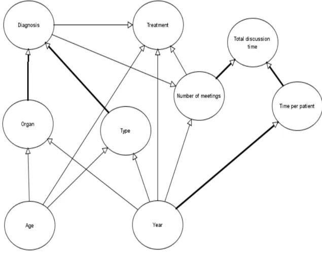
6.3! Hypothetical links and structure hypotheses ... 93!
6.4! Parameters and explanation of data ... 98!
6.5! Selection of plausible relations – three variables ... 100!
6.6! Selection of plausible relations – five variables ... 106!
6.7! Revised model structure ... 109!
6.8! Summary ... 110!
Chapter 7!!Evaluating the Strength of Associations ... 111!
7.1! Impact of MDT meetings ... 111!
7.2! Conditional probabilities from data ... 112!
7.3! Impossible combination and learning conditional probabilities ... 118!
8
7.5! Impact of age on other factors ... 127!
7.6! Efficiency in the MDT meetings with years ... 133!
7.7! Impact of year on type, organ and treatment ... 135!
7.8! Impact of diagnosis on the treatment and number of meetings ... 138!
7.9! Using MDT findings for health care management ... 141!
7.10!!!!Summary ... 141!
Chapter 8!!A Method for Modelling Associations ... 142!
8.1! Modelling Associations ... 142!
8.1.1! Assumptions ... 146!
8.1.2! Modelling issues ... 147!
8.2! Outline of a comprehensive tool ... 149!
8.3! Discussion and related research ... 154!
8.3.1! Medical case studies with related aims ... 154!
8.3.2! Related approaches using Bayesian network modelling ... 156!
8.4! Summary ... 157!
Chapter 9 Conclusion ... 158!
9.1! Review of the research hypotheses ... 158!
9.1.1! Hypothesis 1: the need for new methods ... 158!
9.1.2! Hypotheses 2 & 3: The structure of a BN model from knowledge and data…. … ... 161!
9.1.3! Hypothesis 4: The strength of strong associations ... 162!
9.1.4! Hypothesis 5: A method for analysing observational data ... 162!
9.2! Future work ... 163!
Chapter 10!!References ... 165!
Appendix A Establishing plausible causal relations ... 185!
A.1! Plausible relations - number of meetings, year and diagnosis ... 185!
A.2! Plausible relations - organ, age and year ... 187!
A.3 ! Plausible relations - type, age and year ... 190!
Appendix B!!Evaluating the strength of relations ... 194!
9
B.2! Impact of year on type, organ and treatment ... 195! B.3! Impact of diagnosis on treatment and MDT meetings ... 196!
10
Glossary of Abbreviations
BN Bayesian Network
MDT Multidisciplinary Team
EBM Evidence-Based Medicine
RCT Randomised Controlled Trial
SORT Strength of Recommendation Taxonomy
NICE National Institute for Health and Clinical Excellence
CI Confidence Intervals
BF Bayes Factor
MCID Minimum Clinically Important Difference DAG Directed Acyclic Graph
CPD Conditional Probability Distributions CPT Conditional Probability Table
JPD Joint Probability Distribution
CI Conditional Independence
NPT Node Probability Table
MLE Maximum Likelihood Estimation
EM Expectation-Maximisation
BIC Bayesian Information Criterion AIC Akaike Information Criterion
GS Greedy Search
NPC Necessary Path Condition PBN Prognostic Bayesian Network MCMC Markov Chain Monte Carlo MDL Minimum Description Length BDR Bronchodilator Response
LOS Length of Stay
PBNs Prognostic Bayesian Networks MDL Minimum Description Length BDR Bronchodilator Response
11
TP True Positive
FP False Positive
TN True Negative
FN False Negative
PPV Positive Predictive Value NPV Negative Predictive Value CC Correlation Coefficient
ROC Receiver Operating Characteristic
AUROC Area Under the Receiver Operating Characteristic Curve
12
List of Figures
Figure 2-1 A non MDT process 24
Figure 3-1 A strong association BN formed of four variables 40 Figure 3-2 The probability of ‘High’ sputum for no evidence (in the left
BN) and the probability of ‘High’ sputum for no mechanical ventilation is observed (in the right BN)
43 Figure 3-3 Dynamic discretisation in a continuous node with Normal (5,
1) and Normal (10, 5) 45
Figure 4-1 MDL based PBN to demonstrate the time dependent ordering of variables
61 Figure 4-2 The ROC curve from the independent dataset in [1] 65 Figure 5-1 The process of recommending treatments to patients referred
to the MDT 73
Figure 5-2 Bayesian network model fragment constructed with links based on (a)
84 Figure 5-3 Bayesian network model fragment constructed with a link
based on (b) 84
Figure 5-4 Bayesian network model fragment constructed with a link based on (c)
85 Figure 5-5 Structure of the complete MDT BN model structure from the
links of possible relation types 88
Figure 6-1 BN fragment for learning plausible relations between the
Number of meetings and other variables 94
Figure 6-2 Hypotheses regarding the BN fragment shown in Figure 6-1 95 Figure 6-3 Five BN models for representing five different hypotheses:!!,
!!, !!, !! and !!" regarding the Treatment fragment
97 Figure 6-4 A Bayesian network model for parameter estimation 99 Figure 6-5 Bayesian parameter learning networks for determining the
best structure for the variables Number of meeting, Year and Diagnosis
104
13
Figure 6-6 Structure of the MDT BN model fragment for learning plausible relations between five model variables
107 Figure 6-7 Revised structure of the MDT BN after learning the data
supported relations
110 Figure 7-1 A multinomial BN model for estimating parameters from data 114 Figure 7-2 Underlying expressions used for nodes in a multinomial BN
model
115 Figure 7-3 (a) A multinomial model for learning the probability of each
treatment for benign pancreas 120
Figure 7-3 (b) A multinomial model for learning the probability of each treatment for malignant pancreas
121 Figure 7-4 A graphical representation of the model to test the hypotheses
of interest. Left-hand and right-hand sides of the graph are identical, and each corresponds to parameter estimation part for the relevant strong association link of the BN model depicted in Figure 6-7
124
Figure 7-5 An example of actual Bayesian network to test the hypothesis of interest to the clinicians, e.g. if cancerous organs were high in an older age group (i.e., 46to54) than in a younger age group (i.e., under 46)
125
Figure 7-6 Number of patients per cancerous organ for each of the seven age groups
128 Figure 7-7 Geometric mean of BFs to assess a) changes that occur in
each organ for other age groups in relation to a particular age group and b) a change that occurs in each organ for an older age group when compared with younger age groups
130
Figure 7-8 Number of patients per cancer type for each of the seven age groups
132 Figure 7-9 Geometric mean of BFs to assess a) changes that occur in
each type of cancer for other age groups in relation to a particular age group and b) a change that occurs in each type of cancer for an older age group when compared with younger age groups
132
Figure 7-10 Geometric mean of BFs to assess efficiency in the MDT meetings with years
134 Figure 7-11 Changes with years a) in Type, b) in Organ and c) in 137
14
Treatment
Figure 7-12 Evidence for a difference that occurs a) in surgery and b) in each meeting category for each diagnosis category compared to others
140
Figure 8-1 A flow chart of modelling association 145
Figure 8-2 Time needed to calculate a parameter mode 148
Figure 8-3 (a) How to construct a strong association BN structure using knowledge and data
150 Figure 8-3 (b) How to evaluate strong association strength and address
relevant queries
151 Figure 8-4 Changes that occur in the quality of food with the level of
danger
152 Figure 8-5 Changes that occur in the low quality of food for the Medium
and High danger levels compared to the Low level
15
List of Tables
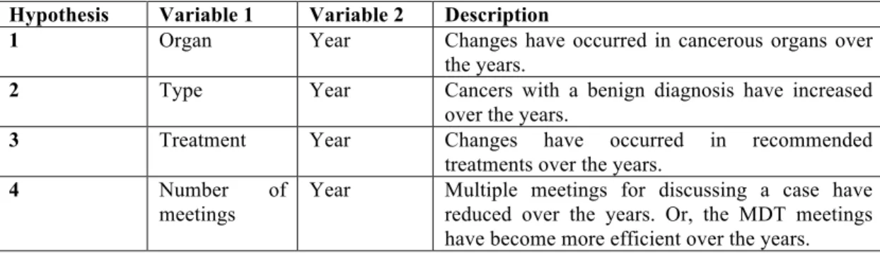
Table 1-1 Research hypotheses verified in this thesis 20
Table 2-1 Jefferys’ scale of evidence for Bayes factors 36
Table 3-1 Methods of Bayesian net inference 46
Table 4-1 Measures for evaluating the ability of a Bayesian network 64 Table 4-2 Evaluation methods and measures for BNs discussed in sections
4.1.1 to 4.1.3 67
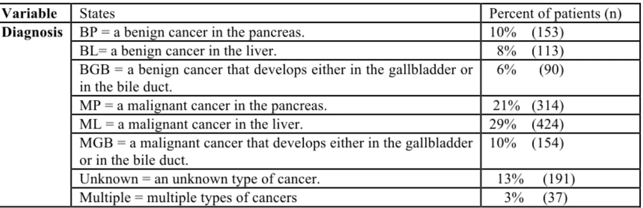
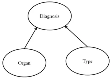
Table 5-1 Possible categories of cancer for each organ 75
Table 5-2 Summary statistics of the MDT meetings for the study period 76 Table 5-3 The distribution of values of the Age, Year and Number of
meetings for patients in the ‘Meeting data’ 80
Table 5-4 The distribution of the values of the Organ and Type for patients in the ‘Organ-Type data’
80 Table 5-5 The distribution of values of the Diagnosis for patients in the
‘Diagnosis data’
81 Table 5-6 The distribution of values of the Treatment for patients in the
‘Treatment data’ 81
Table 5-7 Relation types that exist between the model variables 82 Table 5-8 Hypotheses for the relations between other variables and Age 86 Table 5-9 Hypotheses for the relations between other variables and Year 86 Table 5-10 Hypotheses for the relations between other variables and
Diagnosis
87 Table 5-11 Hypothesis for the relations between Treatment and Number of
meetings 87
Table 6-1 Hypotheses of the variables for the fragments relating to Organ and Type
94
Table 6-2 Hypotheses that do not appear in Figure 6-3 98
16
patients of each Year and Diagnosis combination
Table 6-4 Probabilities of data points obtained per learned parameter for !!
of the Number of meetings fragment 104
Table 6-5 Joint probability and score per hypothesis per fragment 105 Table 6-6 Normalised scores of the sixteen competing hypotheses one of
which assumes to be the best in terms of the data
109 Table 7-1 Counts of the cancerous organ for patients in the corresponding
age group
113 Table 7-2 Probability of each cancerous organ given the age group 116 Table 7-3 Probability of each cancer type given the age group 116 Table 7-4 Probabilities over the states of a) Organ, b) Type, c) Number of
meetings and d) Treatment given year
117 Table 7-5 Probability of each meeting category given Diagnosis 117 Table 7-6 Counts of the recommended treatments for patients in the
corresponding diagnosis option
118 Table 7-7 Probabilities over the states of Treatment given diagnoses 122 Table 7-8 Results per hypothesis test. A positive BF from a test indicates
evidence to support an increase for the corresponding organ for the 46to54 age group compared with the under 46 age group
126
Table 7-9 BF obtained for each organ from a hypothesis testing whether there is an increase for an older age group compared with a younger age group
126
Table 7-10 BFs (with two decimal places) that derive from the hypothesis tests for meeting categories 1 to 4 and more, for the five years considered
133
Table 8-1 BFs to assess changes in food quality according to the level of
danger 151
Table 8-2 The results produced in [2] 155
Table A-1 The posterior probability of each data point for each learned parameter of H2:Number of meetings is dependent on Diagnosis and Year
185
17
parameter of H3:Number of meetings is dependent on Year Table A-3 The posterior probability of each data point for each learned
parameter of H4:Number of meetings is dependent on Diagnosis
186 Table A-4 The cancerous organs for patients corresponding to the age group
and year combination
187 Table A-5 The posterior probability of each data point for each learned
parameter of H1: Organ is independent of Age and Year
188 Table A-6 The posterior probability of each data point for each learned
parameter of H2: Organ is dependent on both Age and Year
188 Table A-7 The posterior probability of each data point for each learned
parameter of H3: Organ is dependent of Age
189 Table A-8 The posterior probability of each data point for each learned
parameter of H4: Organ is dependent of Year
190 Table A-9 The cancer severity stages for patients corresponding to the age
group and year combination
190 Table A-10 The posterior probability of each data point for each learned
parameter of H1: Type is independent Age and Year
191 Table A-11 The posterior probability of each data point for each learned
parameter of H2: Type is dependent on Age and Year
192 Table A-12 The posterior probability of each data point for each learned
parameter of H3: Type is dependent on Age
192 Table A-13 The posterior probability of each data point for each learned
parameter of H3: Type is dependent on Year
193 Table B-1 Bayes Factors (BFs) to analyse the impact of Age on Type 194
Table B-2 BFs to analyse the impact of Year on Type 195
Table B-3 BFs to analyse the impact of Year on Organ 195
Table B-4 BFs to analyse the impact of Year on Treatment 196
Table B-5 BFs to analyse the impact of Diagnosis on Surgery 196 Table B-6 BFs to analyse the impact of Diagnosis on Number of meetings 197
18
Chapter 1
Introduction
Clinicians and other health care professionals use research studies to understand the domain. The design of a study is considered to be crucial for determining the strength of the evidence resulting of the study. Experimental studies such as randomised controlled trials (RCTs) use randomisation to decrease the effect of confounding, and provide the highest ranked evidence. Due to this most attention has been given to experimental trials rather than observational studies. However, experimental trials are not suitable for all questions of interest, and in addition, are sometime impossible to conduct since the time and cost require are often very high. Thus, an important research challenge within the health service domain for today is to produce strong evidence from observational studies.
Every study uses a technique for assessing the strength of the results that it generates. For observational studies, two common techniques are: using P values, and Confidence Intervals. Both these statistics state if the result derived from the hypothesis tests it is statistically significant. Some judgments are then made by experts to determine how likely a change can be made on the basis of this evidence. This process can become difficult since studies reporting these measures rarely indicate how they should assist in managing complex issues.
The analysis of observational data requires the use of a model, such as a multivariate regression. Bayesian networks (BNs) are well known as expert systems but can also be used to model data. A BN is a probabilistic model that represents the probabilistic relationships and conditional dependencies among variables. A BN allows probabilistic inference to be performed coherently, using the law of probability. Also a BN has the
19
capability to represent associations elicited from experts as well as from data, and this makes it perfectly suitable for causal modelling.
Many BNs have been developed to provide support to various clinical tasks including diagnosis, treatment selection, risk analysis and health care management [3][4][5][6][7][8]. However, their application to regular practice is still rare. Numerous studies have mentioned the existing methods for justifying the use of BNs appeared to have drawbacks [9][10]. Specifically, these methods are mostly for showing how accurate a BN model is in predicting the states of one outcome whereas in most health care domain the existing framework of clinical evidence from observed data is for providing decision support to queries regarding multiple outcomes. This thesis proposes a novel way to use a BN model to address clinical queries. . The initial interest here is to form a BN model for representing causal relations by combining the knowledge of experts and data found from an observational study.
Unlike most approaches, there is no need to construct a full model, instead the relations for each variable can be considered in turn to establish if the knowledge based causal relation show the plausibility of existence for the available data. Secondly, this thesis proposes to use the data of plausible relations of the BN model for assessing the strength of each of these relations. Further, it demonstrates that Bayesian analyses on findings from this assessment generate evidence, allowing more confident support for queries by health professionals.
The method is introduced using a case study and data collected from meetings of a Multidisciplinary Team (MDT) meeting process that treats patients suffering with cancer or suspected to have cancer. Data about the MDT meeting process were collected from the Barts and the London HPB (HepatoPancreaticoBiliary) centre following some changes to the MDT process. By evaluating the strength of each of the associations, we examine whether the MDT process has improved treatment recommendations for these patients.
20
1.1
Hypothesis
The thesis is about using a BN to combine the use of both knowledge and data to answers clinical queries. In particular, the thesis addresses the five research hypotheses listed in Table 1-1.
Table 1-1 Research hypotheses verified in this thesis
Hypothesis Chapter of
the thesis
It is important and possible to answer clinical queries from observational data.
It is important to propose a new method for answering clinical queries that derive from observational studies.
2, 3, 4
Data, if available, can demonstrate existence of associations in an expert constructed causal Bayesian Network model
6 Using both the knowledge of experts and data from an observational study we can form a BN to represent associations between its variables.
5, 6 For the BN model we can assess the strength of each association. The results from this assessment can then help to address a relevant query with confidence.
7 The above techniques have the potential for successfully analysing observational data found outside the clinical domain
8
1.2
Structure of this thesis
Chapter 2 discusses the potential benefits of Bayesian methods for introducing new changes in health service. We review the existing approaches to examine the effectiveness of complex health care initiatives and discuss the pitfalls of these approaches.
Chapter 3 introduces BNs and reviews existing methods for their construction, including both expert judgement and learning from data. The importance of dynamic
21
discretisation which extends the use of BNs to continuous variables is described. Then, the chapter highlights existing techniques to complete a BN’s construction process. Chapter 4 reports on the existing applications of BNs to medical and health care domain. The chapter surveys the types of application in the health care domain and the associated techniques of evaluation and their limitations. Overall, this survey shows that the existing techniques for using BNs in this domain are not sufficient for our aim: the analysis of non-experimental data.
Chapter 5 introduces the case study. The chapter identifies the factors relevant for the problem domain, including the assumptions that a health professional might wish to confirm. Then, drawing on existing work, it presents an initial BN for the domain that was constructed by consulting with an expert. This BN contains causal relations and is the starting point of our analysis.
The next three chapters present the main contribution of the thesis.
Chapter 6, working with the case study shows how the expert-judged causal relations in the initial BN can be assessed against data, and the results can be used to ensure that the structure of the BN model given in Chapter 5 represents only those associations that both experts and data have confirmed.
Chapter 7, again using the case study, shows how to assess the strength of each expert and data based association of the BN model and to use the results to address queries. The chapter shows how to construct the posterior distribution over the parameters of each association from data, using an auxiliary multinomial BN model. Further, it shows how this model can be used to answer questions about the modelled domain, using a Bayesian approach to uncertainty and confidence.
Chapter 8 presents the complete methodology for the analysis of data, in a way that could be applied to other studies. The chapter shows that the approach is not restricted to the domain of the case study used but can be applied to successfully model associations in any domain.
22
Chapter 2
Clinical Evidence in Health Services
Introducing changes in health service is a challenging task. It takes time, collaborative effort and energy. Before implementation it is essential to ensure that this change is in the best interest of patients, will improve the quality of care, clinically-led and based on the best available clinical evidence. Many health professionals now seek knowledge from scientific research to make their decisions on organisational design. Marston et al. categorised these studies into six study types: descriptive, taxonomic, analytics, interpretive, explanatory, and evaluative [11].
In evidence-based approach, the best way to assess the effect of an intervention is to perform a randomized controlled trial [12]. When the change in health service concerns introducing a complex intervention such a multidisciplinary team which varies in composition, frequency, and processes, this is difficult to conduct [13]. In [12] Boxer et al compared the intervention group with a non intervention group to evaluate the performance of such an intervention, and acknowledged that the approach generates bias.
Identifying factors which impact on intervention effectiveness and understanding possible disadvantages of the intervention is also not simple from research studies. Altman [14] stated that a large proportion of published medical research lacking either relevance or sufficient methodological rigour to be reliable enough to answer clinical questions. Classical measures showing associations between factors such as P-values and Confidence Interval (CI) values are hard to interpret [15][16][17]. In contrast, Bayesian inference is advantageous since it allows expertise, or prior evidence, to be integrated with evidence from data.
23
In this study we examine the potential benefits of Bayesian methods for introducing new changes in health service. We review the existing approaches to examine the effectiveness of complex health care initiatives and discuss the pitfalls of these approaches.
2.1
Introducing organisational changes in
health services
In health services managers and health professionals regularly take challenging initiatives to make useful organisational changes. For patients suffering with complex illness such as cancer and mental illness, many have focused on replacing existing recommendation process with Multidisciplinary Team (MDT) Meetings intervention.
What is an MDT?
MDT is the short word for ‘multidisciplinary team’. The key idea of an MDT is that different hospital specialists work together to provide care for a patient. In each MDT meeting the team discuss patients and make decisions about the next stage of their care [18].
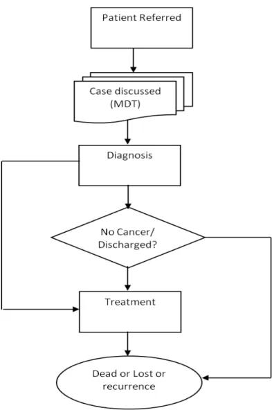
A patient journey in the MDT arm
For a complex disease like cancer GP refers the patient to a clinic/hospital. During the clinic visit specialists examine symptoms, test results and other relevant factors to understand the current state of the disease. After diagnosis, the patient is discussed at an MDT meeting where doctors, specialist nurses, the oncologists, surgeons, radiologists and pathologists meet to discuss the specific case, and consider the scans, general health of the patient, the type of the cancer and the wishes of the patient to decide an appropriate course of treatment.
What is involved in the non-MDT process?
In a non-multidisciplinary setting a GP can provide health care to patients. Figure 2-1 provides a simplified overview of the pathways followed in general practice to provide effective treatments to patients.
24
In brief, after seeing a patient presenting with signs and symptoms, a GP may follow (a) the history of the patient, (b) any presented complain, (c) the outcomes of test(s), or (d) all listed options for diagnosis. The GP applies the diagnostic label to justify a decision to prescribe a treatment option. If no treatment is needed then the GP may discharge the patient or sent him back home to monitor. For a complex diagnostic label, the GP may decide to refer the case to a specialist in a hospital. This referral often initiates the MDT process for recommendations.
Figure 2-1 A non MDT process
Evaluating the impact of MDT
As MDT meetings require substantial administrative, human and technical resources to run successfully, it is important for the meetings to run well[19]. The following questions can therefore be used for evaluating MDT meetings:
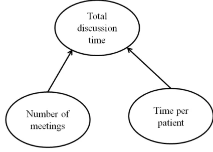
! How long does it take to discuss each patient? ! At how many meetings is each patient discussed?
Patient'
GP#
Diagnosis
Treatment
Monitor
Discharge
Outcome
Referral
25
! Is the decision correct?
In [12] Boxer et al compared MDT and non MDT groups patients to understand the pattern of care for those suffering with lung cancer and reported decreased diagnosis to surgery time, more recommendations of radiotherapy (66% versus 33%, P <0.001), chemotherapy (46% versus 29%, P < 0.001), and palliative care (66% versus 53%, P < 0.001). In [20] authors reported better treatment recommendations in the MDT group (76.81% patients underwent neoadjuvant chemotherapy instead of direct surgery). In [21] the use of a multidisciplinary breast cancer evaluation programme provided important second opinions for many and led to a change in treatment recommendation for 43% (32 of 75) of the patients. In [22] authors compared the treatment of patients with inoperable NSCLC before and after the introduction of MDT, and found that the introduction of an MDT was associated with an increase in the proportion of patients being staged and a change in treatment; more patients received chemotherapy and fewer received palliative care only.
In addition to the benefits in treatment recommendations, MDT discussion can facilitate faster initial of treatment [23], reduce hospitalisation time and costs [24][25], and improve coordination of care[26]. Many authors have shown that patients who received multidisciplinary care were significantly more satisfied than others [27][28]. Also in most situations patients prefer to visit once to a clinic and receive care provided by a team of specialists then a multiple-visit approach [23].
A number of the above studies are based on before and after design [29]. Since care for cancer patients is improving over time, it may be possible that patents for recent times were staged more accurately than those diagnosed before [12]. Some MDT related research studies have shown the benefits of MDT meetings by conducting multiple concurrent organisational changes such as centralising the process [30], increasing caseload [31], and appointing new specialists [32]. Despite these adjustments the evidence for implementing an MDT process is compelling. The question of ones interest is now how to implement this process change and this is what addressed in the empirical part of the thesis.
26
2.2
Causality
The term causality is about investigating that a cause is something that produces an effect. For the time-series data in Economics, Grenge [33] formulated causality as this - a ‘cause’ ought to improve our ability to predict an effect in a probabilistic system. In this discipline the use of structural equation models has been seen as the dominant approach to making inference about causal effects. An example of causality from Medicine is that the establishment of specific bacteria is the cause of specific infectious diseases. In Statistics a probabilistic cause is one that increases or reduces the chance that the effect will occur, and a probabilistic statement about a cause and effect gives quantitative information about an estimate of the strength and nature of that relation. It also provides quantitative information on potential effect modification and about any relation that may exist between the cause and its effect [34].
Experimental studies, such as Randomised Controlled Trials (RCTs) often provide the most trustworthy methods for establishing causal relations from data. In an experimental study (a) the analysis of causation begins with studying the effects of causes, (b) effects of causes are always relative to other causes – it takes two causes to an effect and (c) not everything is taken as a cause so focus is always on some specific fields. Such studies, while potentially highly informative, may be:
• Impossible, impractical or unethical. For example, to assess the effectiveness
of photodynamic therapy (PDT) it is impossible for the clinicians to allocate the patients with brain tumours into a PDT group and a placebo group [35].
• Unnecessary if the effect of a treatment is very high. For example, the use of
Imatinib (Glivec) to treat patients with Chronic Myeloid Leukaemia [36].
• Inadequate. In an RCT, the patients who participate must meet the chosen
study criteria and the follow-up period is short, whereas the treatment evaluated takes place in clinical practice – where a large quantity of patients suffering from many different conditions are of concern – for a longer period
27
of time. Thus, the estimate of an effect of a treatment which was found in the RCT may not be externally valid or generalisable outside the context of the trial [37] [38].
• Increases the type-1errors – false positive errors – due to interim analyses.
During an ongoing experiment, an interim analysis of data is held to let the investigators know whether the intervention is efficient or harmful in relation to the current placebo in order for them to decide if the study should be stopped earlier than planned. In any situation, an interim analysis that is held but hasn’t been planned in advance increases the type-1 error [39].
Causality to nonrandomised observational studies has also been investigated extensively. Observational studies are based on observed data, and these data are more readily available than experimental data. As observational data become increasingly available, opportunities increases for using them. Besides, observed data describe situations that happened in the past and there are no needs for doing experiments. These make applications of observational studies higher where generalisation is an issue during discovery of causal relations or simply statistical associations.
2.2.1
Causal DAG
Directed acyclic graph (DAG) models are well-used tools for capturing causal relationships and for guiding attempts to discover these relations from data. They supply a means of extracting causal conclusions from probabilistic conditional independence properties inferred from purely observational data.
A DAG consists of nodes that represent variables, and arrows that join these variables. Given a joint distribution over an ordered set of random variables (!!,…,!!), one can construct an associated DAG with the (!!) as vertices by adding arrows to !!!!(!= 0,..,!−1) from the smallest subset, !!, of all earlier variables, !! = !
!,…,!! , such
28
!!!! !!|!
!
According to Hernan and Robins [40], a causal DAG is a DAG in which:
i. the lack of an arrow from !! to !! can be interpreted as the absence of a direct causal effect of !! on !! (relative to other variables on the graph)
ii. the inclusion of the measured variables implies that the causal DAG must also include unmeasured common causes.
One description of the idea of 'cause' relates it to an intervention or forced changes. If A causes B, then forcing A to a new value causes B to change. This is relevant to decision making when there is a need to change B but it cannot be done directly. Pearl [41]and other have popularised causal modelling and have developed a principled way to predict the outcome of interventions. These models assume that the direction of causal relations is known from some source other than data.
Also, with two variables A, B, it is not possible to tell from data (i.e. statistics) whether A causes B or B causes C or neither. The third cases arises from a possible unknown third variable U, which causes both A and B and therefore give rise to a correlation between A and B.
2.3
Frequentist inference and interpretation
In the frequentist method, an investigator performs a statistical test – e.g. a hypothesis test – on a sample of a target population and uses the results of the test to make inference about the population. The method mostly utilizes P-values and confidence intervals (CIs) to measure the results of the test. Because these measures are easy to misinterpret they can easily lead to an invalid conclusion when a clinician considers them to decide on clinical application [15]. I discuss about the use of the measures of frequentist more in Sections 2.3.1 and 2.3.2. In contrast to the frequentist method, the Bayesian methods of statistical inference are rather simple and highly applicable
29
alternative for assessing the results of statistical tests [42]. This method is described in Section 2.4.
2.3.1
Null hypothesis, P-values and Confidence intervals
The frequentist method uses hypothesis tests and considers the null hypothesis. For a hypothesis such as: is chemotherapy with surgery more effective as a treatment for the patients with stomach cancer than the chemotherapy alone, the null hypothesis,!!, particularly states: there is no difference in effect between the treatment options. An investigator tests a null hypothesis by calculating the P-value.
There are many definitions available for a P-value.These definitions are placed in relation to either the test of significance of Ronald A. Fisher or the hypothesis testing method of Jerzy Neyman, and Egon S. Pearson. Here we have given two definitions to demonstrate the difference:
“The P-value is the probability of observing data as extreme as, or more extreme than, the data actually observed assuming that the null hypothesis is true”. [43]
“A p-value is the probability of finding a result as extreme, or fantastic, or disappointing, as the one return by a statistical test”. [44]
A P-value of 0.05 is the cut-off for rejecting or not rejecting the null hypothesis [45][46]. If the measured P-value of the test is below the cut-off it indicates that the result is statistically significant [47] – that is, considering the hypothesis above, any difference in effect between the treatment options is likely to be real and not to have occurred by chance [48]. Conversely, a P-value which is equal or greater than 0.05 informs the investigator that the evidence is not sufficient to reject the null hypothesis so the result of the test is not statistically significant and any difference may be due to chance.
However, a P-value less than the cut-off point is not the evidence to support the hypothesis. According to Akobeng [45], a “p-value of <0.05 should not be regarded as
30
‘proof’ that an intervention is effective, and a p-value of ≥0.05 does not also mean that the intervention is not effective”. Further, the P-value does not give information about whether the result of the test is suitable to be placed into clinical practice. Many have therefore suggested that a study should use confidence intervals (CIs) to determine the clinical importance of the result [42]. There are now also requirement that to submit a clinical paper the authors must include both CIs with the P-values in their results [49][50].
A CI measures the significance of a result and the magnitude of effect of the intervention that is under consideration [42]. Instead of defining a probability, the CI estimates a range of plausible values within which the ‘true’ value is expected to be observed, and the use of the 95% CI, the measure that is most common in the studies, indicates that 95 out of 100 times the true value lies within the range [15]. The width of the CI can indicate (1) the precision of an estimate – the narrow the CI the better is the precision – and, (2) the amount of error in an estimate.
As a method of reporting the statistical significance of results, CIs are known to be easier than a P-value.[45]. In brief, along with the information about the statistical significance, a CI helps an investigator to determine when an effect is clinically important [48] [51][52].
2.3.2
Criticisms of the use of P-values and CIs
The use of both P-values and CIs have been criticised for their improper use and misinterpretation with regards to the results of clinical research studies.
In [53], Steven has stated twelve misconceptions that exist among investigators when they decide to interpret a P-value that arises from a two-group randomized controlled trial. Some of these misconceptions also exist among the investigators when they interpret the P-values that arise from an observational research study. Fenton and Neil [54] also present a summary of the problems with the use of P-values, drawing on the book The Cult of Statistical Significance [55]. This thesis includes some of the criticisms which the authors of the above studies have mentioned, and in addition,
31
included few more that other researchers have made during their discussion regarding the use of the P-values and CIs.
Specifically, the following criticisms are found regarding the use of P-values:
• Provides misinterpreted assessment of the null hypothesis.
If a P-value is 0.05, an investigator often misinterprets the result stating that there is a 5% probability that the null hypothesis or no relation is true [56][57]. However, R.A Fisher has introduced the P-value as a rough numerical guide which one can follow to evaluate the strength of evidence against the null hypothesis. His proposal in relation to a P-value less than 0.05 was to suggest an investigator to repeat the test and make conclusions based on the results of subsequent tests. Besides, it is not possible to equate the P-value with the probability of the null hypothesis since an investigator only calculates the P-value considering that the null hypothesis is true [56].
• Makes one to focus less on the problem of interests.
A smaller P-value is only to show more evidence against a null hypothesis. But from an investigator’s point of view the exclusive focus on the null hypothesis is not always interesting [54]. Goodman [58] demonstrates that deriving the strongest evidence sometimes requires a different scope, addressing a question that needs a composite hypothesis in order to answer it properly.
• Generates confusion because the use of cut-off level is arbitrary.
A P value of < 0.05 is commonly taken as statistically significant, but the use of this threshold for the P-value has been considered to be arbitrary [46][59]. For an investigator it is difficult to propose an interpretation of a P-value that is near to 0.05; it turns out that during an interpretation any previous evidence or the judgment influences the suggestion. For example, if a P-value is 0.06, the value is a short distance from the significant level and therefore, the investigator can suggest the interpretation that the
P-32
value is showing is that the result is almost statistically significant or he can simply say that there is no evidence of a relation [42].
• Accelerates inconclusive assessment of clinical relevance.
The P-value does not provide the information that is more important to a clinician, namely, the clinical significance or relevance of a relation [54]. What clinicians are interested in is to know about the magnitude of an effect and therefore, they can intuitively misinterpret statistical significance as clinical significance.
• Provides wrong interpretation of the used data.
“The P-value is not the probability of the observed data under the null (chance) hypothesis, because the P-value includes the probability of more extreme data”. [56]
• Provides misleading information for the tests of significance.
Two tests based on the same observed data do not always give us the same P-value [58]. Goodman [56] has further demonstrated that if two trials are run, and the sizes of the trials are the opposite – one is large whereas the other is small, even if the P-values for both are 0.05 the evidence against the null hypothesis in these cases will be different. This tells us that an investigator’s assumption that the identical data means the identical evidence will not always be acceptable.
• Overemphasised on the use of the cut-off level.
When interpreting the P-value the investigator’s emphasis on the 0.05 threshold value is regarded more strongly than it should be [60]. Since a P-value of 0.05 only corresponds to the minimum Bayes Factor (we will discuss more about Bayes Factor in Section 2.3) of 0.15, it represents at best moderate evidence against the null hypothesis. Sterne et al. [46] have mentioned that a strong evidence against the null hypothesis comes from a P-value which is much smaller than 0.05.
33
• Inappropriate for an inductive inference.
The P-valuesrepresent deductive inference [42]; a hypothesis is initially held and tests are then performed to check if the observations are consistent with the hypothesis [61]. In contrast, strong association inference in clinical practice requires inductive inference where the clinicians first make observations and then decides which hypothesis is likely for the observations [62]. Since their interest is in knowing the probabilities of effects based on the observed data, the clinicians often incorrectly interpret P-values using inductive inference [61][63].
• Suitable only to support dichotomous outcome.
The emphasis of a P-value is on the strength of evidence considering that only dichotomous ‘reject’ or ‘fail to reject’ outcomes.
The criticisms made regarding the use of CIs are as follows:
• For the 95% CI, an investigator often interprets this to imply that there is a 95%
probability that the true relation lies with the 95% CI [64].Whereas what 95% actually means is that when the same test is repeated many times and the CI is calculated for each, then 95% of such intervals will include the true relation [64], and many clinicians ignore this distinction during their interpretations.
• While making an interpretation, clinicians do not always consider the
implications – the importance for applying into clinical practices – of the range of values in the interval [46]. They prefer to use CIs to examine significance and the 95% CI usually uses P < 0.05. A relation is classified as significant when the 95% CI excludes the null hypothesis of no relation [15]. Regarding this drawback with CIs, Goodman [61] states “their impact on the interpretation of research is unclear”.
• Clinicians do not always prefer to make healthcare decisions with 95%
34
association between the factors. For example, a clinician may be interested in knowing whether an intervention has an 85% probability of showing an effect.
• The use of a CI can lead to a misleading conclusion. With the reference to the
study [65] Shakespeare et al. [15] explained that the results given suggesting the effect is not being statistically significant, do not rule out a potential benefit completely and therefore that, a conclusion of ‘no effect’ is misleading.
• The relationship between the width of a CI and the sample size of the test is not
always linear; in general, investigators need to increase the sample sizes by a factor of four to halve the width of the CIs [51]. Therefore, if a clinician intuitively thinks that a linear relation exists, erroneous decisions can result.
2.4
Bayesian inference
Bayesian inference method can overcome many limitations of the frequentist and offer many advantages when it comes to evaluating the strength of evidence. In particular, these advantages can be summarised by the following points:
• Bayesian inference calculates the evidence in favour of a null hypothesis
[66][60][67].
The usual interpretation of significance tests can be used only to reject hypotheses and do not offer an assessment of the strength of evidence in favour of the null hypothesis. Bayesian methods of statistical inference let us calculate what is really required as evidence – including the cumulative impact of different evidence – and this is not
35
Here, !!(!) specifies the prior probability regarding the uncertainty for the hypothesis and ! !! !) is the likelihood of data which specifies the probability of the data given the hypothesis. These two then combine in Bayes’ Theorem to give ! !! !) which is the posterior probability of the hypothesis given the observation that is made from the data.
• It can handle uncertainty in moeling and draw inference about a relation.
While investigating the effect of one variable on another one needs to think about several other possible covariates. It is not often clear if the chosen set is the right set of covariates, and this confusion generates uncertainty that should be taken into account during this investigation. Similarly, other functional and distributional assumptions may lead to different estimates of quantities of interest, and again, one would like to take account of uncertainty about these assumptions within the estimation process. The Bayesian inference method allows doing this in a natural way by averaging over the candidate models with their posterior probabilities as weights [66][57][68].
• By giving the probability for a hypothesis on the basis of the data Bayesian
methods permit inductive inference, which are more appropriate for assessing cause-effect relations. [62][69].
• During hypothesis tests, the use of Bayesian methods enable a researcher to
measure the strength of the evidence by calculating Bayes factors (BFs) [56][61][70].
A Bayes Factor (BF) is the ratio of the probabilities of two competing hypotheses. For example, if we have two hypotheses:!!! and !!, the BF computes by taking the ratio of
the conditional probability of the hypothesis, !!, given the data ! and the conditional probability of the competing hypothesis, !!, given the same data !!, from the equation as follows:
36
When the priors for the hypotheses – ! !! and !(!!) – are equal, the Bayes factor of
two competing hypotheses is
In words,
Posterior odds = Bayes factor × prior odds
The use of Bayes factor can quantify the evidence for one hypothesis relative to another [71] and can suggest which hypothesis is better for predicting the data that an investigator observes. According to Goodman [58], the use of Bayes factors lets the investigator make a clearer distinction between evidence and error, and enables him to derive a proper measure for the evidence. The magnitude of the Bayes factor calculated from the observed data also informs us about the strength of the evidence [56]. For this purpose, Jeffreys [72] has recommended a scale (Table 2-1); an interpretation of the Bayes factor based on the scale helps to decide whether the data we have to hand support one hypothesis over another and in what degree.
Table 2-1 Jefferys’ scale of evidence for Bayes factors
Bayes factor Strength of Evidence > 100 Decisive evidence for !!
30 - 100 Very Strong evidence for !!
10 - 30 Strong evidence for !!
3 - 10 Substantial evidence for !!
37
According to the scale, if the Bayes factor for !! against !! is 1.5, and then the interpretation indicates that the observed data are 1.5 times likely to have occurred under the hypothesis !! than under the hypothesis !! . This BF corresponds to the
category: Anecdotal evidence for!!!, which specifies that although the BF favours the hypothesis!!!, we do not have strong evidence from the observed data to reject or accept either hypothesis.
The use of Bayes Factor provides the flexibility – such as linking evidence, supporting the rare co-ordination – during Bayesian analysis. In particular, these advantages can be summarised by the following points:
• A large number of hypotheses is sometime needed to test a complex
relationship. To determine the strength of the relations results from all these tests needed to be used to ensure a complete assessment. An investigator can take the cumulative of the BFs from the tests during an analysis.
• A large P-value can tell that the result found is not statistically significant. But
one can simply find a large P-value just because there is less or no indication of that particular relation in the available data. The use of priors allows taking account of this uncertainty within the Bayes Factor.
2.5
Summary
This chapter examines the potential benefits of Bayesian methods for introducing new changes in health service. It reviews the existing approaches to examine the effectiveness of complex health care initiatives and discuss the pitfalls of these approaches.
38
Chapter 3
R
eview of Bayesian N
etworks
The chapter discusses the basic components of Bayesian Networks (BNs). The chapter starts with an introduction to BNs and then discuses, in Section 3.1.1, how a BN can model both discrete and continuous variables. Section 3.1.2 discusses the methods developed to perform inference in a BN. Section 3.2 provides a review of the methods used to construct a BN, with Section 3.3 covering the tools available for constructing BNs.
3.1
Introduction to Bayesian networks
The theory of BNs has been developed since the early 1980s, building on early work by Pearl [41], Jensen [73], Lauritzen and Spiegelhater [74] and others.
A BN, also known as a causal probabilistic network or a belief network, is a graphical model that represents probabilistic relationships among a set of variables. They consist of two parts: a graphical structure and a set of parameters. The structure is to represent a directed acyclic graph (DAG) and the parameters are to determine the Conditional Probability Distributions (CPDs) for the variables.
The structure of a BN is formed by the variables – known as nodes – and links that connect the variables. The variables represent the factors (or the propositions) that we find as relevant for the domain being modelled and the links convey information about dependency relations between the variables. Usually, the relations within the structure are expressed by using the wording of family relations: for example, to describe the
39
relation formed by the link from a variable X to another variable Y, we often prefer to say that X is a parent of Y or Y is a child of X.
The purpose of the Conditional Probability Distributions (CPDs) in a BN is to quantify the strength of the relationships that are defined within its structure. The Conditional Probability Distributions can be defined as: (a) Conditional Probability Table (CPT) – for discrete variables and (b) Conditional Probability Distributions (CPD) –for the continuous variables. The BN that has both discrete and continuous variables is known as a ‘Hybrid Bayesian Network’ [75]. The CPD of a variable has a collection of parameters, the number of parameters being determined by the type of considered variable.
Figure 3-1 is a BN for the diagnosis of pneumonia. This model is based on the discussion in [76], but represents the development of the disease in a simplified manner. Since all the links of the BN are chosen to show that the parent variables have strong influence on the child variables, this can be regarded as a Bayesian Network representing strong associations. For example, the link Pneumonia → Fever shows that
Pneumonia is a cause for Fever. The BN has two parents for the variable Sputum;
Pneumonia and Mechanical ventilation regard as two separate, but interrelated, causes for increased (High) production of sputum.
40
Figure 3-1 A BN formed of four variables
One important property of BNs is their ability to represent the Joint Probability Distribution (JPD) for all the variables in a compact form [77]. The traditional approach, i.e. the chain rule, requires a full specification of the probability distributions. In this traditional approach, the full JPD of a probabilistic model with ! random variables!!,!!,….,!! is as follows
This approach is complex and has the potential to introduce a high number of probability entries [78]. In contrast, the framework of a BN reduces the complexity inherent in the full joint probability distribution by reducing the number of probabilities
41
of an inference. In particular, given the structure, the JPD for the BN is the product of all conditional probabilities specified in the BN:
where !"!(!!) are the parents of variable !! in the BN. The conditional probabilities are
therefore determined by !(2!"!! !!) parameters instead of !(2!) that they would
otherwise require if the JPD were computed directly using Equation 3.1. Using Equation 3.2, the BN saves (a) the space that requires for storing the parameters and (b) the time that requires for computations.
Based on the BN in Figure 3-1 the JPD by using Equation 3.1 computes as:
Considering the necessary conditional independence assumptions, the JPD by using Equation 3.2 computes as:
This representation allows us to determine the conditional probabilities for the large CPT, i.e. the CPT for the variable Sputum, with 2!!! i.e. 8!parameters rather than 2!
i.e.,16 that is required otherwise.
42
Before entering any evidence, based on the prior probabilities on variables, the probability that a patient is producing high sputum is 74.5%. We can calculate this using equation 3.6.
If we get the information that the patient is not receiving mechanical ventilation than this situation will reduce the probability of producing high sputum to 0.55 from Equation 3.7.
43
This probability is lower than earlier one, since we are now sure that the patient did not receive any mechanical ventilation. The right side BN in Figure 3-2 demonstrates that the evidence we enter into Mechanical ventilation does not cause any change in
Pneumonia since the variables are conditionally independent given Sputum.
Figure 3-2 The probability of ‘High’ sputum for no evidence (in the left BN) and the probability of ‘High’ sputum for no mechanical ventilation is observed (in the right BN)
3.1.1
Static and dynamic discretisation methods
A BN can include both discrete and continuous variables [75]. A discrete variable has a finite, usually small, set of discrete values and in contrast, a continuous variable has an infinite number of values: that is, the variable can take any value between any two points on a scale. However, BNs generally require a continuous variable to be discredited in order to reduce the number of distinct values by dividing its whole range into a finite set of disjoint intervals [79].
44
Discretisation methods mainly fall into two types, namely: static discretisation and dynamic discretisation. In a static method, the intervals do not change: that is, remain static, while in a dynamic method the intervals change depending on the assignment of probability. Traditionally, a static discretisation is performed in two steps: 1) the user defines the number of intervals for the range of the given continuous variable and 2) the set of cut-off points is then determined in order to assign the probabilities. There are a number of methods that can help users to make the best choice when defining the number of intervals [80][81]. In [81], Clemen has explained ‘the bracket median method’ where the values of a continuous variable are divided into ! equal- width intervals and the median of each of the intervals is used to label the interval. In each of the ! intervals the assigned probability is!1/!.
The number of intervals used influences the accuracy of a BN [82] [83] and also for the level of complexity for a computation [84] – resulting in a longer time to calculate the conditional probabilities in the BN as the number of intervals increases. As a result, to limit the complexity, a user likes to define a minimum number of intervals; this leads to more intervals in the areas where the probability is expected to be varying fastest and fewer, wider intervals where the probability is expected to be more nearly constant. Since in a static method the user would have to understand in advance what the probabilities will be in each area of the range, this leads to more intervals than are essentially required [82].
In [84], Kozlov and Koller attempted to overcome the limitations of static discretisation methods and described a dynamic discretisation method instead. The work shows that an iterative algorithm that can be used to perform discretisation, varying the intervals depending on the evidence observed. Another dynamic discretisation method was later proposed by Neil and his colleagues [79], and the general outline of the method can be found in [83] [79]. In brief, the discretisation starts by considering the whole range of the variable and then recursively divides the range into two intervals until an acceptable level of accuracy is obtained. In each of the iterations the conditional probabilities are calculated and inference is performed to update the probabilities given the observed evidence. Although the method of [79] is influenced by the work of Kozlov and Koller, but the algorithm is simpler and yet capable of achieving higher accuracy.
45
Figure 3-3 demonstrates dynamic discretisation in a continuous node with the distribution Normal (mean=5, variance =1) and the distribution Normal (mean=10, variance=5) with green and blue colour. The node has been discretised following Neil’s method. The result clearly shows wider intervals in those areas where the probability is more constant – at the centre and extremes of the normal – and narrow intervals elsewhere.
Figure 3-3 Dynamic discretisation in a continuous node with Normal (5, 1) and Normal (10, 5)
In general, a dynamic discretisation method let us to model a BN by producing more accurate intervals in the areas that matter the most. In addition to this, the adjustments to the intervals in response to new evidence also help to ensure that a greater accuracy is obtained in the BN. Because of these advantages dynamic methods are most suitable for incorporating continuous variables with those that have discrete states [85], and consequently, have been applied by many to deal with clinical problems where some factors of interests have to be measured using a continuous scale. In this thesis, the BN needs both discrete and continuous variables, so we have preferred to use a dynamic method for discretisation.
46
3.1.2
Inference in Bayesian networks
A Bayesian Network can update the probability of any unknown variable. In particular, given evidence into some variables the model calculates the posterior probabilities for the variable of interest. However, many BNs are complex, which makes it impossible to perform Bayesian inference calculations manually. Due to this, an increasing number of researchers have turned their attention to develop efficient methods of Bayesian inference. Some of the classic methods for exact inference are summarised in Table 3-1.
Table 3-1 Methods of Bayesian net inference
Author Year Description
Perl [86] 1986 A message propagation algorithms whereby the probability distributions for each variable update in response to observations of one or more variables. Pearl’s original algorithm applies only to networks that are trees but similar algorithms have since been used for approximate inference in general BNs.
Shachter [87] 1988 The algorithm reverses links until the explanation of the probabilistic query is obtained from the network Lauritzen and
Spiegelhater [74]
1988 The ‘Junction tree’ algorithm initially transforms the BN into a tree, clustering some variable together. Inference is then done by message passing, using an algorithm similar to Pearl’s.
Zang and Poole [88] 1994 A variable elimination algorithm whereby variables eliminate after summation.
3.2
Construction methods for Bayesian nets
BNs provide an ideal mechanism to model problems that involved uncertainty. At the same time, a network can be formulated to combine all the relevant domain information in an intuitive way. The links can represent cause-effect relations between variables so that it is possible to design the relations in a BN from the understanding of domain experts.