http://eprints.whiterose.ac.uk/97244/ Version: Accepted Version
Article:
Xiangjin B., Chen,, Gao, Jiti, Li, Degui orcid.org/0000-0001-6802-308X et al. (1 more author) (2018) Nonparametric Estimation and Forecasting for Time-Varying Coefficient Realized Volatility Models. Journal of Business and Economic Statistics. pp. 1-13. ISSN 0735-0015
https://doi.org/10.1080/07350015.2016.1138118
[email protected] https://eprints.whiterose.ac.uk/
Reuse
Unless indicated otherwise, fulltext items are protected by copyright with all rights reserved. The copyright exception in section 29 of the Copyright, Designs and Patents Act 1988 allows the making of a single copy solely for the purpose of non-commercial research or private study within the limits of fair dealing. The publisher or other rights-holder may allow further reproduction and re-use of this version - refer to the White Rose Research Online record for this item. Where records identify the publisher as the copyright holder, users can verify any specific terms of use on the publisher’s website.
Takedown
If you consider content in White Rose Research Online to be in breach of UK law, please notify us by
ISSN: 0735-0015 (Print) 1537-2707 (Online) Journal homepage: http://amstat.tandfonline.com/loi/ubes20
Nonparametric Estimation and Forecasting for
Time-Varying Coefficient Realized Volatility Models
Xiangjin B. Chen, Jiti Gao, Degui Li & Param Silvapulle
To cite this article: Xiangjin B. Chen, Jiti Gao, Degui Li & Param Silvapulle (2016):
Nonparametric Estimation and Forecasting for Time-Varying Coefficient Realized Volatility Models, Journal of Business & Economic Statistics, DOI: 10.1080/07350015.2016.1138118
To link to this article: http://dx.doi.org/10.1080/07350015.2016.1138118
Accepted author version posted online: 25 Mar 2016.
Submit your article to this journal
Article views: 2
Nonparametric Estimation and Forecasting for Time-Varying
Coe
ffi
cient Realized Volatility Models
Xiangjin B. Chen1, Jiti Gao1∗, Degui Li2 and Param Silvapulle1
1Monash University, Australia and2University of York, United Kingdom
Abstract
This paper introduces a new specification for the heterogeneous autoregressive (HAR) model for the realized volatility of S&P 500 index returns. In this modelling framework, the coefficients of the HAR are allowed to be time-varying with unspecified functional forms. The local linear method with the cross-validation (CV) bandwidth selection is applied to estimate the time-varying coefficient HAR (TVC-HAR) model, and a bootstrap method is used to con-struct the point-wise confidence bands for the coefficient functions. Furthermore, the asymp-totic distribution of the proposed local linear estimators of the TVC-HAR model is established under some mild conditions. The results of the simulation study show that the local linear estimator with CV bandwidth selection has favorable finite sample properties. The outcomes of the conditional predictive ability test indicate that the proposed nonparametric TVC-HAR model outperforms the parametric HAR and its extension to HAR with jumps and/or GARCH in terms of multi-step out-of-sample forecasting, in particular in the post-2003 crisis and 2007 GFC periods, during which financial market volatilities were unduly high.
Keywords: Bootstrap Method, Heterogeneous Autoregressive Model, Local Linear Estimation, Locally Stationary Process, Nonparametric Method, Time-Varying Coefficient Models. JEL Classifications: C14, C22, C52, C58, G32
∗Correspondence to: Jiti Gao, Department of Econometrics and Business Statistics, Monash University, 26 Sir
John Monash Drive, Caulfield East, Victoria 3145, Australia.. Email: [email protected].
1
Introduction
Financial return volatility is fundamental to portfolio diversification, pricing financial assets and derivatives, and risk management, among others. As a consequence, volatility modelling and forecasting have been two of the most researched topics in both theoretical developments and practical applications in financial econometrics. Engle (1982) and Bolleslev (1986) developed ARCH/GARCH models for deterministic volatility modelling of financial market, which led to various extensions and empirical applications in the last three decades. Recently, several authors studied the GARCH model with time-varying coefficients (TVC). For example, Frijns et al. (2011) introduced a TVC-GARCH model based on multinormial switching mechanism, while Polzehl and Spokoiny (2006) proposed an adaptive procedure to estimate the GARCH coefficients as a function of time. In addition, Heston (1993), Ruiz (1994), and Jacquier et al. (1994) developed stochastic volatility models in both the continuous and discrete time series frameworks. In these models, however, the volatility is assumed to be a latent factor and the daily volatility series are estimated largely from daily return series.
The seminal papers by Andersen and Bollerslev (1998) and Andersen et al. (2001), among others, introduced the nonparametric realized volatility (RV) measures constructed from intra-day transaction data, which retain most of the pertinent information for measuring, modelling, and forecasting RV over the daily and long horizons. Additionally, RV was shown to be an efficient and consistent estimator of the latent volatility of asset returns series. Evidently, the availability of nonparametric measures of latent volatility constructed from high frequency intraday data such as the RV has created a new innovative research direction on the modelling and forecasting of volatil-ity in the recent literature on financial econometrics. The construction of observable RV series and the use of standard time-series techniques have led to promising approaches for modelling and forecasting daily return volatility.
The RV is known to possess the long memory property, and as a result several studies modelled
the RV as the ARFIMA process, which is known to be difficult for estimating and forecasting. Based on the Heterogeneous Market Hypothesis introduced by M¨uller et al. (1993), as an alterna-tive to ARFIMA model, Corsi (2009) proposed the heterogeneous autoregressive (HAR) model, which is a relatively simple autoregressive specification and shown to capture the crucial long memory feature of the RV series. In spite of its simplicity, Corsi (2009) showed that the HAR model can successfully encapsulate the main empirical features of financial returns distribution’s fat tails and thus has a remarkably better forecasting performance than its competitors. McAleer and Medeiros (2008) provided an excellent literature review and compared the performance of the HAR with that of the latent GARCH-type and stochastic volatility models. The authors further pro-posed a HAR with multiple-regime switching smooth transition model for RV, combining the HAR and the smooth transition autoregressive models. Liu and Maheu (2008) introduced a jump com-ponent as well as asymmetric comcom-ponents to HAR model. See also Raggi and Bordignon (2012) and Nonejad (2014) who proposed various extensions to HAR model for the log-transformed RV (logRV) series.
Corsi et al. (2008) showed that the residual series of the HAR model exhibits volatility cluster-ing and thus proposed HAR-GARCH model to explicitly account for this property. They found that the HAR-GARCH model outperforms the HAR model in terms of out-of-sample point forecasting. Subsequently, the HAR with various jump components in modelling and forecasting the logRV se-ries has received notable attention in the recent literature. Anderson et al. (2007) introduced an HAR-J model, in which the price process includes daily jumps associated with short-lived busts in realised volatility, and proposed an HAR-CJ model, in which logRV is modelled in terms of multi-period rough jumps and smooth continuous components. Some further advances can be found in Bollerslev et al. (2009) and Andersen et al. (2011). These studies raise the HAR model with jumps to the prominence by showing that the HAR models with jump components produce better RV forecasts than those without jump components. In this paper, we propose a flexible data-driven nonparametric approach and apply this to estimate the TVC-HAR model, and compare the results
with those of the aforementioned HAR-type models in terms of out-of-sample forecasting of daily, weekly and monthly logRV.
The principal contributions of the paper are the following: (i) it introduces an alternative speci-fication for HAR model of S&P 500 index returns by allowing the parameters of the HAR model to be time-varying with unknown functional forms; (ii) it applies a local linear smoothing method to estimate the TVC-HAR model and uses a bootstrap method to construct the point-wise confidence bands for the coefficient functions; and (iii) it evaluates the multi-period out-of-sample forecast-ing performance of the proposed TVC-HAR model against the HAR, HAR-GARCH models with and without jumps. To our knowledge, this paper is among the first to generate nonparametric multi-step ahead forecasts for logRV.
In a preliminary analysis of the daily S&P 500 stock index returns over the period 1999-2010, we found that the coefficients of the simple HAR model across the sub-sample periods were sig-nificantly different. Without making any parametric assumption as to the way in which these coef-ficients vary over time, in this paper we allow the coefficients of the HAR models to vary over time with unknown functional forms. If these coefficients are assumed to be constants but indeed time-varying, then the model misspecification can give rise to time-varying volatility for HAR model, which is introduced and extensively studied by Corsi et al. (2008). Thus, the nonparametric TVC-HAR model that we propose in this paper is a natural competitor to the well-known TVC-HAR-GARCH model. To assess the out-of-sample performance of the model proposed in this paper relative to several parametric counterparts, we use the conditional predictive ability (CPA) test developed by Giocomoni and White (2006). We further employ a hypothesis testing method to find supporting evidence for its relative in-sample performance. In this respect, this paper makes methodological as well as empirical contributions to the growing literature on realized volatility.
Modelling the TVC is common in finance. The TVC models have been applied to several ar-eas in finance, including the popular capital asset pricing model and the term structure of interest
various parametric structures to TVC functions, in practice, the underlying true feature of the TVC function is largely unknown. However, the traditional approach to establish a TVC model relies on the assumption made on the parametric functional forms for the time-varying coefficients. More-over, although it is simple to implement, the parametric structure imposed for the TVC functions is often too restricted and can be unrealistic, leading to model misspecification, and thus to inac-curate forecasting. By contrast, without imposing any specific structure, nonparametric estimation of the TVC models would be an attractive alternative, because it allows the data to “speak for themselves”. There exists a vast literature on nonparametric estimation of the mean regression models as well as their econometric applications. For instance, Robinson (1989) contributed to the early development of the nonparametric mean estimation of TVC regression models with exoge-nous explanatory variables, while Cai (2007) and Li et al. (2011), among others, contributed to the recent literature on this topic. Meanwhile, there has also been increasing interest on nonparametric estimation of the dynamic time series models under the assumption of local stationarity (c.f., Kim, 2001; Giraitis et al., 2012; and Zhang and Wu, 2012). However, so far as we know, there is little literature on nonparametric estimation of the TVC realized volatility models with local stationarity assumption. This paper fills this gap by further deriving the asymptotic distribution theory of the proposed nonparametric methodology which is given in the appendix.
The rest of the paper is organized as follows. Section 2 introduces the TVC-HAR model specification for logRV, local linear estimation method with the cross-validation (CV) bandwidth selection and the construction of the point-wise confidence bands for the coefficient functions, and conducts a simulation study for assessing the finite sample performance of the proposed model and estimation approach. Section 3 provides a description of the parametric and nonparametric out-of-sample forecasting and evaluation. Section 4 describes the S&P 500 series and presents a preliminary analysis of the series, followed by the results of local linear estimation and CPA testing of the proposed nonparametric TVC-HAR model. Section 5 concludes this paper. An asymptotic theory for the proposed methodology with some regularity conditions is given in Appendix A.1
and the generalized likelihood ratio test for the simple HAR model against the TVC-HAR model is outlined in Appendix A.2.
2
Model and Methodology
In this section, we first specify the TVC-HAR modelling framework, and then introduce the methodologies including the local linear estimator and the bootstrap method to construct the point-wise confidence bands for the coefficient functions. Furthermore, we also give a simulation study and report the results.
2.1
Specification of the TVC-HAR Model
We start with Corsi (2009)’s simple HAR model, which is defined by
log RVt = β0+βdlog RVt−1+βwlog RVt−5,t−1+βmlog RVt−22,t−1+εt, (1)
wherelog RVt+1−k,t = k−1 log RVt−1+log RVt−2+∙ ∙ ∙+log RVt−k = 1k
Pk
j=1(log RVt−j) is the
k-period normalized realized variation, β0, βd, βw and βm are the four unknown parameters which
are assumed to be invariant over time. We next relax the restriction that the coefficients of the HAR model (1) are constant which might be unrealistic in practical application as mentioned in Section 1. Instead, we allow that the coefficients of the model can vary over the time with certain unknown functional forms, which leads to a flexible TVC-HAR model for logRV.
Before specifying the nonparametric TVC-HAR model, we introduce some notation through the following general TVC autoregressive time series model:
Yt = Xt⊤βt +εt, t =1,∙ ∙ ∙ ,n, (2)
where Xt = 1,Xt,1,Xt,2,∙ ∙ ∙ ,Xt,d⊤are the lagged values of the response variable Ytwith Xt,k = Yt−k
for k = 1,∙ ∙ ∙ ,d,β = β , β ,∙ ∙ ∙ , β ⊤is a vector of unknown functions of time t, and {ε}is a
sequence of stationary errors. As in Robinson (1989), Cai (2007) and Li et al. (2011), we assume that
βt,j =βj(τt),τt =
t
n, t=1,∙ ∙ ∙ ,n, j=0,∙ ∙ ∙ ,d, (3)
where n is the sample size. Such a specification of βt makes it possible to construct a consistent
nonparametric kernel regression estimation of the coefficient functions, via increasingly intense sampling of data points at each point in the interval [0,1].
Let Yt = log RVt, Xt = 1,log RVt−1,log RVt−5,t−1,log RVt−22,t−1⊤ andβt = βt,0, βt,d, βt,w, βt,m⊤
in the model (2), with the coefficient functions replaced with those defined by (3). We then obtain the nonparametric TVC-HAR model for the logRV series through:
log RVt = β0(τt)+βd(τt) log RVt−1+βw(τt) log RVt−5,t−1+βm(τt) log RVt−22,t−1+εt. (4)
The simple HAR model (1) can be seen as a special case of the TVC-HAR model by restricting the coefficient functions to be constants over the time. Furthermore, note that model (4) is different from those in Cai (2007) and Li et al. (2011), as there is a dynamic structure involved in model (4) and the commonly-assumedα-mixing condition may not be satisfied in our setting.
2.2
Local Linear Estimation Method
We next introduce the local linear method to estimate the coefficient functionsβt,j =βj(τt) for j=
0,d,w,m. The local linear method has been employed in the nonparametric regression estimation
in the literature, due to its attractive properties such as efficiency, bias reduction, and adaptation of boundary effects (c.f., Fan and Gijbels, 1996). Assuming each βj(∙) has a continuous
second-order derivative in the interval [0,1], βj(τt) can be approximated by a linear function through the
first-order Taylor expansion:
βj(τt)≃ aj+bj(τt−τ),
where aj = βj(τ), and bj = β′j(τ) which is the first-order derivative ofβj(τ). Thus, the model (4)
can be locally approximated by
log RVt ≃ Xet⊤θ(τ)+εt, (5)
where Xet⊤ = Xt⊤,Xt⊤(τt −τ)⊤ andθ(τ) = β⊤(τ),[β′(τ)]⊤ ⊤. Note that the dimension for Xet and θ(τ) in the above model is 8.
Based on the local approximation (5), we define the locally weighted sum of squares:
n X t=1 log RVt−eX⊤t θ 2 Kh(τt−τ), (6)
where Kh(u) = 1hK(hu), K(∙) is a kernel function, and h = hn > 0 is the bandwidth satisfying the
conditions that h→0 and nh→ ∞as n → ∞. Note that h controls the amount of smoothing used in the local linear estimation. Then,bθ(τ) can be obtained by minimizing the weighted loss function (6) with respect toθ. By some elementary calculation, we may show that the expression ofbθ(τ) is given by bθ(τ)= Sn0(τ) Sn1⊤(τ) Sn1(τ) Sn2(τ) −1 Mn0(τ) Mn1(τ) , (7) where Snk(τ)= 1 n n X t=1 XtXt⊤(τt−τ)kKh(τt−τ), k= 0,1,2, and Mnk(τ)= 1 n n X t=1 Xt(log RVt)(τt −τ)kKh(τt −τ), k=0,1.
The local linear estimate ofβ(τ)= β0(τ), βd(τ), βw(τ), βm(τ)⊤isbβ(τ) which consists of the first 4
elements ofbθ(τ), and the local linear estimate of the derivativeβ′(τ) isbβ′(τ) which consists of the last 4 elements ofbθ(τ). Proposition 1 in the appendix shows that the local linear estimationbβ(τ) is asymptotically normally distributed under some regularity conditions.
As is well-known, the local linear estimator is sensitive to the choice of the bandwidth h, and thus it is critical to choose an appropriate bandwidth in empirical applications. In this paper, we apply the commonly-used CV bandwidth choice for the time series case (c.f., H¨ardle and Vieu, 1992). Letbβ−t(τt) be the local linear estimated value ofβ(τt) by using the sample{log RVs: s,t}.
The optimal bandwidth hoptis chosen such that
CV(h)= 1 n n X t=1 h log RVt −Xt⊤bβ−t(τt) i2
is minimized. In Section 2.4 below, we conduct a simulation study to evaluate the finite sample properties of the local linear estimator of the TVC-HAR model with the CV bandwidth selection.
2.3
Construction of the Confidence Bands
For given 0 < α < 1, the (1−α) point-wise confidence bands of βj(∙) at point 0 ≤ τ ≤ 1 can be
defined by
h
bβj(τ)−cα/2(τ)×sd(bβj(τ)), bβj(τ)+cα/2(τ)×sd(bβj(τ)) i
(8) for j= 0,d,w,m, wherebβj(τ) is the local linear estimate ofβj(τ), cα/2(τ) is the upperα/2 percentile
of Qj(τ) = (bβj(τ)−βj(τ))/sd(bβj(τ)) andsd(bβj(τ)) is the standard deviation ofbβj(τ). However, (8)
cannot be directly used to construct the confidence bands of βj(τ) as neither cα/2(τ) norsd(bβj(τ))
is known. We next estimate cα/2(τ) andsd(bβj(τ)) by using the bootstrap procedure. Then, by using
the estimates of cα/2(τ) andsd(bβj(τ)) which are denoted bybc∗α/2(τ) andsd∗(bβj(τ)), respectively, the
(1−α) point-wise confidence bands ofβj(τ) can be obtained by h
bβj(τ)−bc∗α/2(τ)×sd∗(bβj(τ)), bβj(τ)+bc∗α/2(τ)×sd∗(bβj(τ)) i
.
The bootstrap procedure to estimate cα/2(τ) andsd(bβj(τ)) is described as follows.
1. Estimateβt by the local linear smoothing method introduced in Section 2.2, and denote the
resulting estimates bybβt for t= 1,∙ ∙ ∙ ,n.
2. For each t = 1,∙ ∙ ∙ ,n, generate log RVt∗ = Xt⊤bβt +ε∗t, where {ε∗t}nt=1 is sampled from the
centred residuals{eεt}nt=1, witheεt =bεt−bεt,bεt =log RVt−X⊤t bβtandbεt = 1nPnt=1bεt. In practice, ε∗t = eεt ∙ ηt, where {ηt} is a sequence of independent and identically distributed random
variables drawn from a prespecified distribution with mean zero and unit variance, such as
N(0,1). Use the data set{(log RV∗
t,Xt) : t = 1, . . . ,n} to estimate the coefficient functions
and denote the resulting estimator asbβ∗(∙).
3. Repeat Step 2 for B times and obtain B bootstrap local linear estimated values,bβ∗(τ,i),i = 1,∙ ∙ ∙ ,B. The estimate of sd(bβj(τ)) is the sample standard deviation of {bβ∗j(τ,i) : i =
1,∙ ∙ ∙ ,B}and is denoted assd∗(bβj(τ)).
4. For each i = 1,∙ ∙ ∙ ,B, use the sequence {bβ∗j(τ,i)} and sd∗(bβj(τ)) to compute Q∗j,i(τ) =
(bβ∗j(τ,i)−bβj(τ))/sd∗(bβj(τ)), and then obtain the estimate of cα/2(τ), denoted bybc∗α/2(τ), by
calculating the upperα/2 percentile of{Q∗
j,i(τ) : i= 1,∙ ∙ ∙ ,B}.
As in Ter¨asvirta et al. (2010), we let the covariates Yt−k, for k = 1,5,22 in the dynamic
autoregression be invariant when generating bootstrap samples, although other bootstrap methods may also be applicable in our setting. In Section 4, the results of our empirical application show that the above bootstrap procedure works reasonably well. Additionally, we find that the point-wise confidence bands for the coefficient functions of TVC-HAR are sensitive to minor variations to the optimum bandwidth which produces the narrowest confidence bands. The simultaneous confidence bands for the coefficient functions proposed in Zhang and Peng (2010) for the case where the observations are independent does not appear to work well in our setting, where the data is weakly dependent and locally stationary, and they are generally much wider than the point-wise confidence bands. Therefore, in the empirical study presented in Section 4, we report only the point-wise confidence bands.
2.4
Simulation Study
In this section, we conduct a simulation study to evaluate the finite sample behavior of the local linear estimator with the CV bandwidth, which is introduced in Section 2.2, to estimate the coeffi -cient functions of the TVC-HAR model. In this simulation study, we specify the TVC-HAR model as
Yt = β0(τt)+βd(τt)Yt−1+βw(τt)Yt−5,t−1+βm(τt)Yt−22,t−1+εt (9)
where τt = nt, and Yt−k,t−1 = k−1(Yt−1+Yt−2+∙ ∙ ∙+Yt−k) = 1kPkj=1Yt−j, k = 1,5,22 and t =
1,∙ ∙ ∙ ,n. The functional forms forβj(∙), j = 0,d,w,m, are generated as: β0(τ) = 0.1×sin(2πτ),
βd(τ) = 0.1×cos(2.5πτ), βw(τ) = 0.1×cos(2πτ), andβm(τ) = −0.1×sin(πτ). We consider two
data generating processes: DGP 1 and DGP 2. In DGP 1,εt in (9) isN(0,1); and in DGP 2,εt is
Student-t with 5 degrees of freedom. We set n = 250, 500 and 1000 sample sizes, and M = 500 replications. Moreover, to ensure that the initial values for the DGP do not affect the results, we generate n+n∗observations, with n∗= 1000 being the burn-in sample size.
The simulation study is conducted in the following steps:
1. Set n= 250 and generate{εt}fromN(0,1).
2. Generate the initial values of the elements of{Y0,Y−1,Y−2, ...,Y−21}.
3. Generate a T×1 series of Yt recursively from DGP1: TVC-HAR with the known coefficient
functions and the standard normalεt.
4. Then, construct the RHS dynamic variables 1,Yt−1,Yt−5,t−1,Yt−22,t−1as defined above.
5. Discard the first n∗ observations of Y
t and Xt, where Xt = (1,Yt−1,Yt−5,t−1,Yt−22,t−1). Use
the remaining n observations to estimate the four unknown coefficient functionsβ(.)j by the
local linear method with the CV bandwidth, and denote the resulting estimates bybβj(.) for
j=0,d,w,m.
6. Repeat the above Steps 3 to 5 M times.
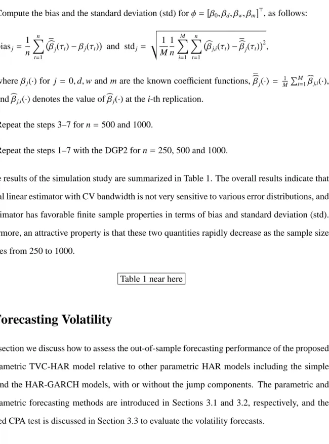
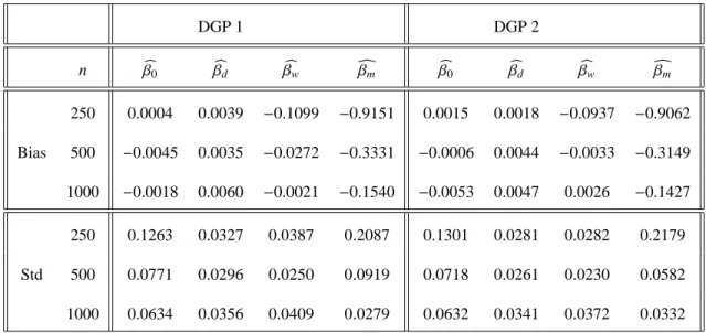
7. Compute the bias and the standard deviation (std) forφ= β0, βd, βw, βm⊤, as follows:
biasj = 1 n n X t=1 bβj(τt)−βj(τt) and stdj = v t 1 M 1 n M X i=1 n X t=1 bβj,i(τt)−bβj(τt) 2 ,
whereβj(∙) for j = 0,d,w and m are the known coefficient functions,bβj(∙) = M1
PM
i=1bβj,i(∙),
andbβj,i(∙) denotes the value ofbβj(∙) at the i-th replication.
8. Repeat the steps 3–7 for n=500 and 1000.
9. Repeat the steps 1–7 with the DGP2 for n=250, 500 and 1000.
The results of the simulation study are summarized in Table 1. The overall results indicate that the local linear estimator with CV bandwidth is not very sensitive to various error distributions, and this estimator has favorable finite sample properties in terms of bias and standard deviation (std). Furthermore, an attractive property is that these two quantities rapidly decrease as the sample size increases from 250 to 1000.
Table 1 near here
3
Forecasting Volatility
In this section we discuss how to assess the out-of-sample forecasting performance of the proposed nonparametric TVC-HAR model relative to other parametric HAR models including the simple HAR and the HAR-GARCH models, with or without the jump components. The parametric and nonparametric forecasting methods are introduced in Sections 3.1 and 3.2, respectively, and the so-called CPA test is discussed in Section 3.3 to evaluate the volatility forecasts.
3.1
Parametric Multi-Step-Ahead Forecasting
In this section we first provide a summary of some selected parametric forecasting models of the logRV series, and then describe how to generate the multi-step-ahead forecasts of logRV using these models.
Andersen et al. (2007) extended Corsi (2009)’s daily HAR model to longer horizons, i.e.,
log RVt,t+δ=βδ,0+βδ,dlog RVt−1+βδ,wlog RVt−5,t−1+βδ,mlog RVt−22,t−1+εt,t+δ, (10)
Theδ-step-ahead forecasts of logRV can be generated as the one-step-ahead forecast from model (10) for a givenδ. The estimates of the parameters in model (10) are expected to vary for different
δ. In this paper, for the purpose of forecasting comparison, we include the parametric HAR-family including simple HAR, HAR-GARCH(1,1) with normal errors, and HAR-J and HAR-CJ models (Equations 13 and 28 in Andersen et al. (2007), respectively), and HAR-J with GARCH(1,1) errors, where the letter C refers to the log continuous sample path component variation, while the letter J refers to the log jump component of logRV.
To generate multi-step-ahead out-of-sample forecasts, we partition the total data sample of size
n into two periods: an estimation period and an evaluation period:
t = 1,2,∙ ∙ ∙ ,k, | {z } estimation period k+1,k+2,∙ ∙ ∙ ,n | {z } evaluation period .
Next, we describe the out-of-sample forecasting methodology only for the HAR model (10), and the methodology is similar for other parametric HAR-type models included in this forecasting exer-cise; see also Andersen et al. (2007) for HAR models with jumps. We generate the volatility point forecasts using a rolling window of fixed length k with the estimation scheme. At the time point
k, let the estimators of parameters in model (10) bebβk
δ,j estimated using the first k observations,
and then the δ-step-ahead out-of-sample forecasts are generated and compared to the realization log RVk+δ. Similarly, at the time point k + 1, bβkδ,+j1 are obtained using the k observations ending
at k+ 1, the second set of δ-step-ahead forecasts are generated and compared to the realization
log RVk+δ+1, and so on. This iterative procedure generates m ≡ n−δ −k+1 number of
out-of-sample forecasts and relative forecast errors. Following Patton (2011), we measure the relative forecast error using the simple mean squared error loss function. In summary, settingδ =1,5 and 22 as the daily, weekly and monthly forecasting horizons, respectively, the conditional forecasts of log RVt,t+δat any time point t ∈ {k,k+1,∙ ∙ ∙ ,n−δ+1}, are computed directly as follows:
E(log RVt,t+δ|Ft)=bβtδ,0+bβ
t
δ,dlog RVt−1+bβtδ,wlog RVt−5,t−1+bβtδ,mlog RVt−22,t−1
forδ =1,5 and 22, whereFtrepresents the information set available up to time t.
3.2
Nonparametric Multi-Step-Ahead Forecasting
The nonparametric multi-step-ahead forecasting for non-linear autoregression models with order d can be made by estimating the conditional meanE(Yt+δ|Yt,∙ ∙ ∙ ,Yt−d+1) via nonparametric
smooth-ing of Yt+δ on (Yt,∙ ∙ ∙ ,Yt−d+1) directly (c.f., Robinson, 1983; H¨ardle and Vieu, 1992; Ter¨asvirta
et al., 2010). The direct nonparametric approach, however, ignores the substantial information contained in the intermediate variables Yt+1,∙ ∙ ∙ ,Yt+δ−1about the conditional mean. Hence, to
im-prove this estimator, Chen et al. (2004) introduced a multi-stage nonparametric predictor, which utilises information in pseudo observations Yt∗+1,∙ ∙ ∙ ,Yt∗+δ−1 (which will be defined later) to gen-erate an estimate for Yt+δ. They showed that such multi-stage smoother improves the estimation
of the conditional mean, and demonstrated that this new predictor is more efficient than the direct nonparametric smoother. In the empirical application, we thus employ the multi-stage nonpara-metric predictor introduced by Chen et al. (2004) for the conditional forecasts of log RVt+δunder
the nonparametric TVC-HAR modelling framework (4), with adjustments made to the predictor to account for the time-varying nature of the coefficient functions. The approach of the nonparametric multi-step-ahead forecasting is described as follows.
1. Choose the optimal bandwidth h by the CV selection introduced in Section 2.2, where
only the first k observations of{Yt,Xt}are used.
2. For one-step-ahead forecast at time t, use the optimal bandwidth hoptfrom Step 1 and obtain
the local linear estimatesbβt,j ofβt,j, using the past observations up to time t. Use thesebβt,j
and model (4) to predict Yt+1, denoted asbYt∗+1, and compare it to the realization log RVt+1.
3. For two-step-ahead forecast at time t, update the vector of regressor values by including the pseudo observationbY∗
t+1. Then, estimate the coefficient functions using the same bandwidth hopt, and let the resulting estimator bebβt+1,j. Use this estimator to generate the
two-step-ahead forecast,bYt∗+2, and compare it to the realization log RVt+2.
4. Similarly, for δ-step-ahead forecast at t, update the set of regressors by adding the pseudo observationsbYt∗+1,∙ ∙ ∙ ,bYt∗+δ−1. Estimate the coefficient functions in the updated model using the same bandwidth hopt and let this estimator bebβt+δ−1,j. Use this estimator to generatebYt∗+δ
and compare it to the realization log RVt+δ.
For simplicity, in Steps 2–4, we apply the same optimal bandwidth, hopt, which is constructed
from Step 1. In practice, however, one may re-estimate the optimal bandwidth hopt, as it may differ
as the data sample changes. The advantage of bandwidth re-estimation is the gain in the forecast accuracy (which may not be significant), but it comes at a cost of a significant increase in the computation time for nonparametric forecasting.
3.3
Evaluation of Volatility Forecasts: CPA Testing
It is of practical importance to evaluate and compare the out-of-sample forecasting performance between the proposed TVC-HAR model and its competitors including the simple HAR and the HAR-GARCH models. To achieve this, we employ the CPA test introduced by Giacomini and White (2006).
Diebold and Mariano (1995) and West (1996) (henceforth referenced as DM-W), contributed to the early literature on the unconditional out-of-sample predictive ability evaluation of forecast-ing models. However, the recent CPA test provides a framework for an unconditional forecast evaluation criterion, which is robust to misspecified forecasting models. In our forecast evaluation which involves three models, the proposed TVC-HAR and the simple HAR are nested models, whereas the proposed TVC-HAR and HAR-GARCH are non-nested models. The CPA test has an advantage over the DM-W approach in that the former is well suited for evaluating CPA of nested as well as non-nested forecasting models. In addition, the CPA test can be applied to multi-step point, interval, probability or density forecast valuation for a general loss function. Furthermore, the CPA approach accommodates conditional forecast evaluation objectives (which is more ac-curate at a specific future date), as well as nesting the unconditional objectives (which is more accurate on average) of the DM-W approach. Although both the unconditional and conditional approaches are informative, the global (or average) relative forecasting performance may conceal important information about the relative forecasting performance over time. Hence, the use of the CPA test appears promising for assessing the merit of the TVC-HAR model against the parametric HAR-type models in terms of out-of-sample forecasting accuracy. The CPA test is implemented via the following three steps.
1. Based on the rolling samples of fixed length k, the conditional forecasts of Yt+δ by using
the TVC-HAR and the benchmark models (say, the simple HAR model), respectively, for a given setFt (defined in Section 3.1), are generated for the target date t+δof the evaluation
period at t = k,k+1,∙ ∙ ∙ ,n−δ. LetbY1,t+δandbY2,t+δbe the conditional forecasts of Yt+δby
using the simple HAR and TVC-HAR models, respectively.
2. For each of the two forecasting models, generate a sequences of losses, Lj,t+δ= L(Yt+δ,bYj,t+δ),
with j=1 denoting the benchmark model, and j=2 denoting the TVC-HAR model, where
through calculating∆Lt+δ = L1,t+δ−L2,t+δ.
3. To test whether the alternative TVC-HAR model outperforms the benchmark model, we consider testing
H0∗: E[∆Lt+δ|Ft]= 0 a.s., versus H1∗ : E[∆Lt+δ|Ft]>0 a.s.
We use the test statistic Tk,m = mZ ⊤
k,mbΘ−m1Zk,m, where Zk,m = m1 Pn−t=kδZt+δ, Zt+δ = πt∆Lt+δ,
m=n−δ−k+1,πt is a chosen test function,
b Θk,m= 1 m n−δ X t=k Zt+δZ ⊤ t+δ+ 1 m δ−1 X l=1 wm,l× n−δ X t=k+l [Zt+δZt⊤+δ−l+Zt+δ−lZ⊤t+δ],
and wm,lis a weight function such that wm,l → 1 as m→ ∞for each l= 1,∙ ∙ ∙ , δ−1.
With respect to the choice of πt, as discussed in Giacomini and White (2006), πt is chosen
by researchers to include variables that are considered helpful to distinguish the relative forecast performance of the two competing models. It can be an indicator of past relative performance (such as lagged loss differences or moving averages of past loss differences) or business cycle indicators, see Bierens (1990) and Stinchcombe and White (1998) for various ways of choosing the test function. Section 4.3 below will specify the choices ofπt and wm,l in the analysis of the
logRV of the S&P 500 index returns.
The null hypothesis H0∗ of equal conditional predictive ability of the models is rejected when
Tk,m > χ2q,1−α, whereχ2q,1−α is the (1−α) quantile of the χ2q distribution and q is the dimension of πt. This rejection occurs when the out-of-sample loss difference{∆Lt+δ} is significantly different
from zero. Furthermore, in case where the null hypothesis of equal conditional predictive ability is rejected, Giacomini and White (2006) also proposed an approach to make forecasting model selection decisions. Their approach consists of the following three steps.
1. Regress ∆Lt+δ on πt over the out-of-sample period for t = k,k+ 1,∙ ∙ ∙ ,n− δ, and let bϕm
denote the regression coefficient matrix. Apply the above χ2
q test and if the null hypothesis
is rejected, then we proceed to step 2.
2. ApproximateE[∆Lt+δ|Ft] usingbϕ⊤mπt, and model A (the benchmark model), with the lower
loss, is considered superior ifbϕ⊤
mπt < c, and model B (the alternative TVC-HAR model) is
superior otherwise. In this paper, we specify c = 0, as we desire to choose a model that yields lower loss at t+δ.
3. Compute the ratio m1 Pn−t=kδI{bϕ⊤mπt > 0}, the relative out-of-sample performance of models A
and B, where I{∙} is an indicator function. Thus, model A is a better forecasting model at
t+δif the ratio<0.5, and model B otherwise.
4
Analysis of the US Market Data
4.1
Preliminary Analysis of the Data
The primary data set consists of tick-by-tick transaction prices for the S&P 500 index for the period from 10/May/1999 to 26/October/2010. All the index data have been supplied by the Securities Industries Research Centre of Asia Pacific (SIRCA) on behalf of Reuters, with the raw index data filtered prior to the construction of the RV data. Construction of RV does not impose any particular requirement on the way in which prices are sampled as long as the corresponding returns are non-overlapping and span the time period of interest. There are variety of different sampling schemes used in the literature. However, it is well established that ultra high-frequency returns would lead to bias in the volatility measures, due to market microstructure effects such as the bid-ask bounce, stale prices and price discreteness. These effects cause the observed asset prices to behave differently to the assumptions underlying the construction of RV. In the literature, there is a general consensus that the five-minute interval minimizes the influence of such microstructure
and Bollerslev et al. (2009), we compute the daily realized variance from five-minute logarithmic returns constructed using the nearest price to each five-minute mark. The resulting daily log RVt
time series is displayed in Figure 1.
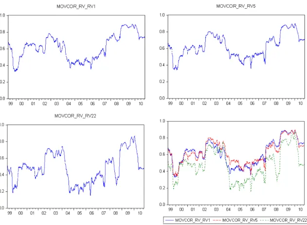
We first fit the simple HAR model (1) to the data set, and the ordinary least squares (OLS) esti-mates of the coefficients are presented in Table 2. All of the coefficients are significantly different from zero at the 10% significance level. Furthermore, to examine if the four coefficients, β0, βd, βw and βm change significantly over time, we also estimate the moving window (with size 250)
bivariate correlations between log RVt and log RVt−1, log RVt−5,t−1, and log RVt−22,t−1, respectively.
All the three sets of correlations are plotted in Figure 2. All three moving window correlations appear to be nonlinear over the sample period and they move in unison over time. In particular, all of the three correlation measures move upwards during the crises such as the 2002-03 stock market downturn and the 2007 global financial crisis (GFC), and then downwards and stay low during the tranquil period between 2003 and early 2007.
Table 2 near here
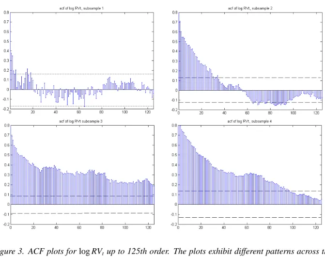
To learn more about the time-varying nature of the coefficients of the HAR models, we subdi-vide the full sample period into four different subsample periods. A simple HAR model is fitted to each of the four subsamples, and the results are also presented in Table 2. Subsample 1 covers the periods before the dotcom crisis, subsample 2 covers the US stock market downturn during the dotcom crisis, subsample 3 covers the period before the GFC, and subsample 4 represents the recent GFC period. The OLS estimates and their standard errors (in the parentheses) of the coeffi -cients in the simple HAR model for each subsample are listed in Table 2. The result of the Wald test for the equality of the regression coefficients indicates that the coefficients are significantly different across the four sample periods, as the value of the test statistic is 61.168. Moreover, the ACF plots of log RVt series for all the four subsamples are presented in Figure 3, which exhibit
different patterns across the subsamples, indicating the dynamic changes of the serial dependence
in the log RVt series. Therefore, from the above our preliminary analysis, the TVC-HAR model
(4) may be a better alternative to the simple HAR specification for the log RVtseries.
4.2
Estimation of the TVC-HAR model
In this section, we implement the methodologies introduced in Sections 2.2 and 2.3 to the logRV of the S&P 500 series. We first compare the local linear estimation method with the Nadaraya-Watson local constant estimation method. The optimal bandwidths chosen by the CV method for the local constant and local linear methods are 0.137 and 0.174, respectively. Overall, the local linear estimates of the coefficient functions are somewhat smoother than those by using the local constant method, mainly due to a slightly larger optimal bandwidth for the local linear method. In addition, as shown in Figure 4, the plot of the residuals from the latter estimation are closer to a normal distribution than those from the former. To evaluate the in-sample estimation performance of the simple HAR model with OLS estimation, the TVC-HAR model with local constant smoothing and the TVC-HAR model with local linear smoothing, the mean squared errors are calculated as 0.269, 0.266, and 0.260, respectively, which indicate that the local linear smoothing method of the TVC-HAR model provides the best estimation overall. Following the preceding observations, we will not further discuss the results of local constant estimation on TVC-HAR.
The local linear estimates of the time-varying coefficient functions in the TVC-HAR models are plotted in Figure 5 along with their 90% point-wise confidence bands. The horizontal lines in all four panels in Figure 5 indicate the OLS estimates: beta0-OLS, beta1-OLS, beta2-OLS and beta3-OLS, respectively of the constant coefficients, β0, βd, βw and βm of the simple HAR
model (1). The plot of the intercept function ˆβ0(∙) in Figure 5 is significantly smaller than the
corresponding constant coefficient during the tranquil period. Thebβd(∙),bβw(∙) andbβm(∙) in Figure
5 are respectively the estimated coefficient functions of log RVt−1, log RVt−5,t−1, and log RVt−22,t−1
on log RVt, Reported along with these estimates are their 90% point-wise confidence bands which
lie either above or below the horizontal lines. The local linear estimates of coefficient functions of TVC-HAR in Figure 5 are denoted by beta0-LL, beta1-LL, beta2-LL and beta3-LL, respectively.
The plot ofbβd(∙) which measures the daily effect of log RVt−1on log RVt is smaller during the
tranquil period, while it is larger during the GFC period. However, the opposite effects emerge from the plot of thebβw(∙) function, which measures the weekly effect of log RVt−5,t−1 on log RVt.
It is larger during the non-crisis period while smaller during the GFC period. The plot of the estimate of monthly effectbβm(∙) shows a downwards trend until 2004 indicating declining effect
of log RVt−22,t−1 on log RVt during this period, reaches its trough during the period 2004–2006,
but then increases on the occurrence of the GFC and peaks around mid-2008 when this crisis was deepening. It is evident that all the coefficients of the HAR model are time-varying.
To find further statistical evidence of whether or not the widely used simple HAR model is adequate for the data, we apply the generalized likelihood ratio (GLR) test proposed by Fan et al. (2001), with the wild bootstrap method to compute the p-value, is outlined in Appendix A.2 below. We use the GLR to test whether H0: simple HAR against H1: TVC-HAR is rejected or not. By
setting B = 200 in the bootstrap procedure, we obtain the p-value of 0, which indicates that the simple HAR model is rejected in favour of the TVC-HAR specification for the logRV of the S&P 500 index returns. Despite the GLR test originally proposed for the independent data, the result of our analysis indicates that this test works well numerically for the weakly dependent and locally stationary logRV series.
4.3
Forecasting and CPA Test
In this section we evaluate the out-of-sample forecasting ability of the TVC-HAR model with the local linear method relative to the simple HAR, CJ, J, GARCH and HAR-J-GARCH models. To do this, we first define the in-sample estimation and the out-of-sample prediction periods as follows:
Evaluation (m)
Estimation (k) pre-GFC post-GFC
Dates 01/07/2002–13/11/2007 14/11/2007–31/8/2008 02/09/2008–16/07/2009
Data size 1345 200 220
The reason for splitting the out-of-sample forecasting period into pre- and post-GFC periods is that during the post-crisis period the stock market volatility has been unduly high. Finding a model that generates superior multi-step-ahead out-of-sample forecasts relative to its competitors during high volatility is very useful to investors and practitioners. To apply the nonparametric forecasting method discussed in Section 3.2, the optimal bandwidth hopt estimated for the full
sample period is used for simplicity and time efficiency. All the models included in this forecasting are estimated using the rolling samples of k observations and the conditional forecasts of log RVt,t+δ
are generated and compared them with the realizations. Following Giacomini and White (2006)’s method described in Section 3.3, we choose the weight function wm,l = 1− δl and the test function πt =(1,∆Lt+δ−1), where∆Lt+δ−1 is the lagged value of the difference of the loss∆Lt+δ, from which
the test statistic for the CPA test is constructed. In what follows, we report the results of the CPA test.
4.3.1 CPA Test of the HAR-type model against the TVC-HAR model
The CPA test applied for testing the H0∗that the parametric HAR-type model (benchmark model)
and the TVC-HAR model have the same out-of-sample forecasting performance against the H1∗
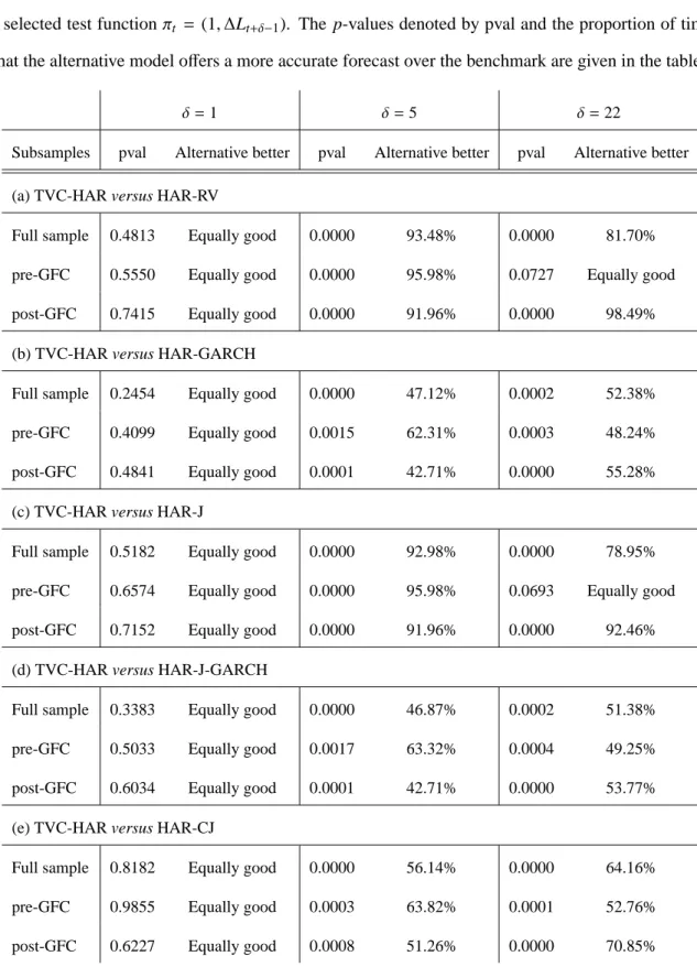
that these two models do not have the same forecasting performance. The p-values of the test statistic are reported in Table 3. Furthermore, the proportion of the times (in percentages) that the alternative model TVC-HAR offers a more accurate forecast over the benchmark model are also reported in this table. When the simple HAR model is considered as the benchmark model, the
results are given in Table 3(a). For the entire forecasting evaluation period, the p-values indicate that the TVC-HAR model is as good as the HAR model in forecasting of log RVt,t+δatδ = 1. On
the other hand, atδ = 5 and 22, the performance of TVC-HAR is superior to HAR in forecasting. The results in Table 3(c) and (e) show that these observations are very similar when the HAR-J and HAR-CHAR-J model are considered as the benchmark model. More importantly, there is an overwhelming evidence showing that the TVC-HAR model consistently outperforms the three HAR-type models in the post-2007 GFC period.
The out-of-sample forecasting evaluations of these models were also made during the 2003 crisis, for which we used the estimation period 10/05/1999–20/09/2001, and the out-of-sample forecasting evaluation periods: pre-2003 crisis period 21/09/2001–16/07/2002 and the post-2003 crisis period 17/07/2002–06/06/2003. The forecasting performance of the TVC-HAR relative to the three HAR-type models are very similar to what was observed during the 2007 crisis. To save space the results for during the 2003 crisis period are not tabulated in this paper.
Table 3 near here
4.3.2 CPA Test for HAR-GARCH and HAR-J-GARCH against TVC-HAR
In this section, the HAR and HAR-J models with GARCH(1,1) errors are treated as benchmark models against the TVC-HAR model. The results of the CPA test are reported in Table 3(b) and (d), respectively, and they show that as a consequence of adding the GARCH component, the out-of-sample forecasting performances of HAR-GARCH and HAR-J-GARECH models have improved for the full forecasting evaluation period, which includes the 2007-crisis. However, it is noticeable that the relative performance of the TVR-HAR model consistently better than the parametric counterparts during the post-GFC period whenδ = 22 and during the pre-GFC period whenδ =5.
5
Conclusions
In this paper, we introduce a flexible TVC-HAR modelling framework for the logRV of the S&P 500 index returns. In this flexible model, the coefficients of the HAR model are allowed to be time-varying with unspecified functional forms, which are estimated by a local linear method. In a simulation study, we find that the local linear estimator for the coefficient functions of a TVC-HAR time series model has good finite sample properties in terms of bias and standard deviation. We construct the point-wise confidence bands for the coefficient functions using the bootstrap procedure, which provide a statistical evidence to show that the HAR coefficients are indeed time-varying. Additionally, the GLR test statistic augmented with the wild bootstrap method is con-ducted to provide further statistical evidence against the simple linear HAR model for logRV of the S&P 500 series in favour of the TVC-HAR model proposed in this paper. We evaluate the multi-step-ahead out-of-sample forecasting performance of the TVC-HAR model relative to the simple HAR model and its extensions to HAR with jumps and/or GARCH. The results of the CPA test developed by Giacomini and White (2006) indicate that the one-step-ahead (daily) forecasting performance of these models are equal. On the other hand, the TVC-HAR model consistently outperforms the other parametric HAR-type models in 5-step-ahead (weekly) and 22-step-ahead (monthly) out-of-sample forecasting, particularly in the post-2003 and 2007 crises periods during which the financial market volatilities were extremely high.
6
Acknowledgements
We are grateful to the Co-Editor–Professor Rong Chen, an Associate Editor and two referees for their helpful comments, which greatly improved the original version of the paper. Thanks also go to the participants of several seminars and conferences for their constructive comments and suggestions on earlier versions of this paper. The authors would also like to acknowledge financial support by the Australian Research Council
Appendix A
A.1. Assumptions and an Asymptotic Distribution
In this part of the appendix, we derive the asymptotic distribution theory of the local linear estimation bβ(τ) defined in Section 2.2, which is of independent interest. Existing literature, such as Robinson (1989), Cai (2007) and Li et al. (2011), mainly considers the limiting distribution of the nonparametric kernel or local linear estimation of the TVC models where the covariates are exogenous and do not include the lagged term of the response. Hence, their results cannot be directly extended to the setting here.
Before giving the asymptotic results, we introduce a general class of evolutionary processes which can accommodate a variety of forms of nonstationary (or locally stationary) behavior. Letτt = nt and
Xt =βt,0+ p P j=1 βt,jXt−j+εt =β0(τt)+ p P j=1 βj(τt) Xt−j+εt, (11)
which allows the autoregressive coefficients to change smoothly over time, and thus provides a much more general framework than the traditional autoregression models. Following Dahlhaus (1996), the process (11) is locally stationary under some mild conditions on the coefficient functions. The locally stationary process behaves like a stationary process in a small neighbourhood of each instant in time, but has a nonstationary behavior globally. We can refer to Kim (2001), and Zhang and Wu (2012) for recent development on nonparametric estimation of the coefficient functions{βj(∙) : 1≤ j≤ p}.
We next convert our TVC-HAR model into the framework of the locally stationary process (11). It is easy to see that model (4) can be re-written as
log RVt = β0(τt)+βd(τt) log RVt−1+βw(τt) h1 5 5 X i=1 log RVt−i i +βm(τt) h 1 22 22 X i=1 log RVt−i i +εt = β0(τt)+hβd(τt)+ βw(τt) 5 + βm(τt) 22 i log RVt−1+ hβw(τt) 5 + βm(τt) 22 iX5 i=2 log RVt−i +hβm(τt) 22 iX22 i=6 log RVt−i+εt ≡ ϕ0(τt)+ 22 X j=1 ϕj(τt) log RVt−j+εt, (12)
whereτt = nt. Hence, the TVC-HAR model falls into the locally stationary modelling framework defined in (11). Before presenting the asymptotic properties of the local linear estimator for the TVC-HAR models, we introduce the following regularity conditions.
Assumption 1. The coefficient functionsβj(∙), j =0,d,w,m, are twicely continuous differentiable in [0,1]. Meanwhile,P22j=0ϕj(τ)zj , 1 for all|z| ≤1+c with c> 0 uniformly inτ∈[0,1], whereϕj(∙) is defined on the right hand side of (12).
Assumption 2. The sequence{εt}is independent and identically distributed (i.i.d.) withE[εt]= 0, 0< σ2 ≡
E[ε2t]<∞andE[|εt|2+κ]<∞forκ >0.
Assumption 3. The kernel function K(∙) is a continuous, symmetric and nonnegative function with a compact support.
Assumption 4. Let the bandwidth h satisfy h→0 and nh→ ∞.
Assumption 1 imposes certain smoothness condition on the coefficient functions which ensures that the local linear approach is applicable and it also entails local stationarity and short-range dependence, respectively (c.f., Dahlhaus, 1996; Kim, 2001; and Zhang and Wu, 2012). The i.i.d. condition on the error term in Assumption 2 can be relaxed to some stationary and weakly dependent conditions such as the stationary martingale differences. Assumptions 3 and 4 are two commonly-used conditions on the kernel function and bandwidth, respectively.
LetFj∗ = ∙ ∙ ∙, εj−1, εjbe a shift process of i.i.d. random variablesεi. We next give the asymptotic distribution for the local linear estimationbβ(τ) defined in Section 2.2, whereτ∈[0,1].
Proposition 1. Suppose that Assumptions 1–4 are satisfied. Furthermore, there exists a measurable and stochastically Lipschitz continuous functionX(∙,∙) such that
max 1≤t≤n Xt∗− X(τt−1,Ft∗−1)=OP 1 n ! , (13)
where Xt∗=(log RVt−1, log RVt−5,t−1,log RVt−22,t−1)⊤. Then, we have √ nhhbβ(τ)−β(τ)−bτ(h) i d −→N0, ν0σ2Σ−τ1 , (14) where bτ(h) = 12h2µ2β ′′ (τ)+oP(h2) with µ2 = R
u2K(u)du, ν0 = R K2(u)du and Στ = E h e XτXe⊤τ i , Xeτ =
Proof. By (13), Assumption 1 and Proposition 4.2 in Zhang and Wu (2012), we can prove that Xt =
(1,log RVt−1, log RVt−5,t−1,log RVt−22,t−1)⊤in the local linear estimation can be replaced byXet =1,X⊤(τt−1,Ft∗−1)⊤,
which would not affect the asymptotic distribution. Noting that {εt} is i.i.d. and εt is independent of
X(τt−1,Ft−∗1), we can complete the proof of (14) by using the central limit theorem and the argument in
Zhang and Wu (2012).
A.2. Specification Testing
In this part of the appendix, we give an outline for the generalized likelihood ratio test developed by Fan et al. (2001) for finding a statistical evidence to check whether the proposed TVC-HAR model fits the data better than the simple HAR model. To outline this test, we consider the null hypothesis:
H0 : β0(τt)=β0, βd(τt)=βd, βw(τt)=βw, βm(τt)=βm,
against the alternative hypothesis:
H1 : βj(τt),βjfor at least one of j=0,d,w,m.
If H0is rejected, then we would infer that the nonparametric TVC-HAR model fits the logRV series better
than HAR. The test statistic is constructed based on the generalized maximum likelihood ratio test proposed by Fan et al. (2001) and defined as follows:
T Sn=
RS S0−RS S1
RS S1
, (15)
where RS S0 is the residual sum of squares under the null hypothesis H0, and RS S1 is the residual sum
of squares under the alternative hypothesis H1. Lettingbβ be the OLS estimate of β = (β0, βd, βw, βm)⊤, then RS S0 = 1nPnt=1bε2t0withbεt0 = log RVt−Xt⊤bβand RS S1 = 1nPnt=1bε2t1withbεt1 = log RVt −X⊤t bβ(τt) = log RVt−Xt⊤bβt.
The null hypothesis is rejected if the p-value of the test is smaller than a nominal level (say 5%). The p-value is computed using the following wild bootstrap procedure introduced by Stinchcombe and White (1998).
1. Under the null hypothesis H0, for each t =1,∙ ∙ ∙,n, generate log RVt∗= Xt⊤bβ+ε∗t, where the{ε∗t}is defined as in Step 2 of the bootstrap procedure in Section 2.3.
2. Use the data set{(log RVt∗,Xt) : t=1,∙ ∙ ∙ ,n}to estimate the models under both H0and H1and then
calculate the corresponding RS S0∗and RS S∗1, and T S∗ndefined in (15).
3. Repeat Steps 1 and 2 for B times and obtain the empirical distribution of T S∗n. Then, the p-value of the test statistics is computed by 1BPBi=1I(T S∗n(i) ≥ T Sn), where I(∙) is an indicator function and T S∗n(i) is calculated as T S∗nby using the i-th bootstrap sample.
References
[1] Andersen, T.G., and Bollerslev, T., 1998. Answering The Skeptics: Yes, Standard Volatility Models Do Provide Accurate Forecasts. International Economic Review, 39, 885−905.
[2] Andersen, T.G., Bollerslev, T., and Diebold, F.X., 2007. Roughing it Up: Including Jump Components in the Measurement, Modeling and Forecasting of Return Volatility. Review of Economics and Statistics, 89, 701−720. [3] Andersen, T.G., Bollerslev, T., Diebold, F.X., and Labys, P., 2001. The Distribution of Realized Exchange Rate
Volatility. Journal of the American Statistical Association, 96, 42−55.
[4] Andersen, T. G., Bollerslev, T., and Huang, X., 2011. A Reduced form Framework for Modeling Volatility of Speculative Prices based on Realized Variation Measures. Journal of Econometrics, 160(1), 176−189.
[5] Bierens, H. B. 1990. A Consistent Conditional Moment Test of Functional Form. Econometrica, 58, 1443−1458. [6] Bollerslev, T. 1986. Generalized Autoregressive Conditional Heteroskedasticity. Journal of Econometrics, 31,
307−327.
[7] Bollerslev, T., Kretschmer, U., Pigorsch, C., and Tauchen, G., 2009. A Discrete-Time Model for Daily S&P 500 Returns and Realized Variations: Jumps and Leverage Effects. Journal of Econometrics, 150, 151−166.
[8] Cai, Z. 2007. Trending Time-Varying Coeffcient Time Series Models with Serially Correlated Errors. Journal of Econometrics, 136, 163−188.
[9] Chen, R., Yang, L., and Hafner C., 2004. Nonparametric Multistep-Ahead Prediction in Time Series Analysis. Journal of the Royal Statistical Society, Series B, 66, 669−686.
[10] Cochrane, J.H., 2001. Asset Pricing. Princeton University Press, Englewood Cliffs, NJ.
[11] Corsi, F., 2009. A Simple Approximate Long-Memory Model of Realized Volatility. Journal of Financial Econo-metrics, 7, 174−196.
[12] Corsi, F., Mittnik, S., Pigorsch, C., and Pigorsch, U., 2008. The Volatility of Realized Volatility. Econometric Reviews, 27, 46−78.
[13] Dahlhaus, R., 1996. On the Kullback-Leibler Information Divergence of Locally Stationary Processes. Stochastic Processes and Their Applications, 62, 139−168.
[14] Diebold, F. X. and Mariano, R. S., 1995. Comparing Predictive Accuracy. Journal of Business & Economic Statistics, 13, 253−263.
[15] Engle R. F., 1982. Autoregressive Conditional Heteroscedasticity with Estimates of The Variance of United Kingdom Inflation. Econometrica, 50, 987−1007.
[16] Fan, J., and Gijbels, I., 1996. Local Polynomial Modelling and its Applications. Chapman and Hall, London. [17] Fan, J., Zhang, C., and Zhang, J., 2001. Generalized Likelihood Ratio Statistics and Wilks Phenomenon. Annals
of Statistics, 29, 153−193.
[18] Frijns, B., Lehnert, T., and Zwinkels, R. C., 2011. Modeling Structural Changes in the Volatility Process. Journal of Empirical Finance, 18(3), 522−532.
[19] Giacomini, R., and White, H., 2006. Tests of Conditional Predicative Ability. Econometrica, 74, 1545−1578.
[20] Giraitis, L., Kapetanios, G., and Yates, T., 2012. Inference on Stochastic Time-Varying Coefficient Models. Working Paper at Queen Mary, University of London.
[21] H¨ardle, W., and Vieu, P., 1992. Kernel Regression Smoothing for Time Series. Journal of Time Series Analysis, 13, 209−232.
[22] Heston, S. L., 1993. A Closed-Form Solution for Options with Stochastic Volatility with Applications to Bond and Currency Options. The Review of Financial Studies, 6, 327−343.
[23] Jacquier, E., Polson, N. G., and Rossi, P. E. 1994. Bayesian Aanalysis of Stochastic Volatility Models (with Discussion). Journal of Business & Economic Statistics, 12, 371−417.
[24] Jagannathan, R., and Wang, Z., 1996. The Conditional CAPM and the Cross-Section of Expected Returns. Journal of Finance, 51, 3−53.
[25] Kim, W., 2001. Nonparametric Kernel Estimation of Evolutionary Autoregressive Processes. Discussion paper 103, Sonderforschungsbereich 373, Berlin.
[26] Li, D., Chen, J., and Gao, J., 2011. Nonparametric Time-Varying Coefficient Panel Data Models with Fixed Effects. The Econometrics Journal 14, 387−408.
[27] Liu, C., and Maheu, J. M., 2008. Are There Structural Breaks in Realized Volatility ? Journal of Financial Econometrics, 6(3), 326−360.
[28] McAleer, M., and Medeiros, M. C., 2008. A Multiple Regime Smooth Transition Heterogeneous Autoregressive Model for Long Memory and Asymmetries. Journal of Econometrics, 147, 104−119.
Challenge to Econometricians. 39thInternational AEA Conference on Real Time Econometrics, 14−15 October 1993, Luxembourg.
[30] Nonejad, N., 2014. Long Memory and Structural Breaks in Realized Volatility: An Irreversible Markov Switch-ing Approach. Available at SSRN 2427675.
[31] Patton, A. J., 2011. Volatility Forecast Comparison using Imperfect Volatility Proxies. Journal of Econometrics, 160, 246−256.
[32] Polzehl, J., and Spokoiny, V., 2006. Varying Coefficient GARCH versus Local Constant Volatility Modeling: Comparison of the Predictive Power (No. 2006, 033). SFB 649 Discussion Paper.
[33] Raggi, D., and Bordignon, S., 2012. Long Memory and Nonlinearities in Realized Volatility: a Markov Switching Approach. Computational Statistics & Data Analysis, 56(11), 3730−3742.
[34] Robinson, P. M., 1983. Nonparametric Estimation for Time Series Model. Journal of Time Series Analysis, 4, 185−208.
[35] Robinson, P. M., 1989. Nonparametric Estimation of Time-Varying Parameters. Statistical Analysis and Fore-casting of Economic Structural Change. Hackl, P. (Ed.). Springer, Berlin, 164−253.
[36] Ruiz, E., 1994. Quasi-maximum Likelihood Estimation of Stochastic Volatility Models. Journal of Econometrics, 63, July 1994, 289−306 .
[37] Stinchcombe, M. B., and White, H., 1998. Consistent Specification Testing with Nuisance Parameters Present Only under the Alternative. Econometric Theory, 14, 295−325.
[38] Ter¨asvirta, T., Tjøstheim, D., and Granger, C. W. J., 2010. Modelling Nonlinear Economic Time Series. Oxford University Press.
[39] Tsay, R. S., 2002. Analysis of Financial Time Series. Wiley, New York.
[40] West, K. D., 1996. Asymptotic Inference about Predictive Ability. Econometrica, 64, 1067−1084.
[41] Zhang, T. and Wu, W., 2012. Inference of Time-Varying Regression Models. Annals of Statistics, 40, 1376− 1402.
[42] Zhang, W. and Peng, H., 2010. Simultaneous Confidence Band and Hypothesis Test in Generalised Varying-Coefficient Models. Journal of Multivariate Analysis, 101, 1656−1680.
Figure 1. Time series of logarithmic realized volatility.
Figure 2. The moving window correlation plots between log RVt and log RVt−1, log RVt−5,
log RVt−22, respectively. The bottom-right plot combines the curves in the other three plots.
Figure 3. ACF plots for log RVt up to 125th order. The plots exhibit different patterns across the
four subsamples, reflecting the dynamic changes of the serial dependency of the log RVtseries over
the sample period.
Figure 4. Plots of the residuals from local linear and local constant regressions as well as their distributions.
Figure 5. The local linear estimates of the coefficient functionsβ(∙) (solid nonlinear line) with 90%
point-wise confidence bands (dotted lines), and OLS estimates (solid horizontal line).