Open Access Dissertations Theses and Dissertations
January 2016
Cardinality Constrained Optimization Problems
Jinhak Kim
Purdue University
Follow this and additional works at:https://docs.lib.purdue.edu/open_access_dissertations
This document has been made available through Purdue e-Pubs, a service of the Purdue University Libraries. Please contact [email protected] for additional information.
Recommended Citation
Kim, Jinhak, "Cardinality Constrained Optimization Problems" (2016).Open Access Dissertations. 1388.
OPTIMIZATION PROBLEMS
A Dissertation Submitted to the Faculty
of
Purdue University by
Jinhak Kim
In Partial Fulfillment of the Requirements for the Degree
of
Doctor of Philosophy
August 2016 Purdue University West Lafayette, Indiana
ACKNOWLEDGMENTS
I have been very fortunate to have two outstanding scholars, Prof. Mohit Tawar-malani and Prof. Jean-Philippe P. Richard as my advisors. Foremost, I express my best gratitude to Prof. Tawarmalani for his unstinted support throughout my Ph.D. study. His astonishing erudition and extraordinary passion have guided me to a stun-ning field, mathematical programming. No one can substitute for his heartfelt effort and ardent guidence for my Ph.D. study. I also would like to show my appreciation to my co-advisor, Prof. Richard for the thoughtful and fruitful advise on my research. I was particularly grateful to his sedulousness and earnestness on commenting my writings and presentations.
In addition to my advisors, I thank two other thesis committee members, Prof. Yanjun Li and Prof. Thanh Nguyen for their comments and questions on the thesis and the defense of the dissertation.
I also would like to acknowledge my family members for their patience, support, and sacrifice. I especially thank my lovely wife Jayoung Sohn for giving me two beloved sons, Timothy and Jeremy during our Ph.D. studies. I am blessed that I have the best women as the sole partner of my life. I next want to appreciate my mother, Yekeum Yoo and my parents in law, Inshik Sohn and Myungna Jeong for their diligence and effort on raising my children. This thesis will never exist without their dedication.
Finally, I gratefully acknowledge the partial support from National Science dation grants CMMI 0900065, 1234897, and 1235236 and a Purdue Research Foun-dation research assistantship.
TABLE OF CONTENTS
Page
LIST OF TABLES . . . vi
LIST OF FIGURES . . . vii
ABSTRACT . . . viii
1 Introduction . . . 1
2 On cutting planes for cardinality constrained linear programming . . . . 7
2.1 Introduction . . . 7
2.2 Disjunctive relaxation of a simplex tableau with a cardinality constraint 9 2.3 A characterization of cl conv(Q) . . . 13
2.4 Dual network formulation of B2 . . . 23
2.5 Label-connected trees and facet-defining inequalities of cl conv(Q0) . 30 2.6 Generalized Equate-and-Relax procedure for CCLPs . . . 38
2.7 Conclusion . . . 49
3 Semidefinite programming relaxations for sparse principal component anal-ysis . . . 51
3.1 Introduction . . . 51
3.2 Characterization of the convex hull of sparse PCA . . . 55
3.2.1 Separation problem . . . 55
3.2.2 Characterization of the convex hull . . . 58
3.2.3 Recovery of an optimal solution . . . 62
3.3 SDP relaxation for sparse PCA . . . 66
3.4 Preliminary computational results . . . 73
3.4.1 pitprops problem . . . 73
3.4.2 Test results with randomly generated matrices . . . 75
3.5 Conclusion . . . 75
4 Facial disjunctive programming formulation and generalized RLT for cardi-nality constrained linear programming . . . 77
4.1 Introduction . . . 77
4.2 Facial Disjunctive Program Formulation . . . 78
4.2.1 Formulation and sequential convexification . . . 78
4.2.2 Finitely convergent cutting plane algorithm . . . 79
4.3 Generalized Reformulation-Linearization Technique . . . 82
4.3.1 Barycentric coordinates . . . 82
Page
4.3.3 Convexification using generalized RLT . . . 87
4.4 Valid inequalities for cardinality constrained knapsack problem . . . 88
4.4.1 Preprocessing . . . 89
4.4.2 Two-term disjunction method: δ-inequalities and its variants 90 4.4.3 Derivation of known inequalities for the literature . . . 102
4.4.4 Derivation of theδ-inequality via lifting. . . 104
4.5 New valid inequalities via lifting . . . 106
5 Concluding remarks . . . 113
5.1 Conclusion . . . 113
5.2 Future research directions . . . 114
LIST OF REFERENCES . . . 116
LIST OF TABLES
Table Page
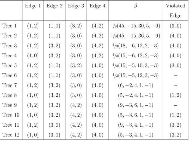
2.1 Feasible spanning trees for Example 4. . . 37
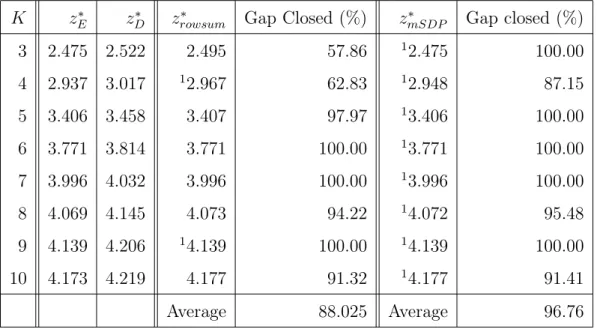
3.1 Optimal values and gaps closed for the test problempitprops . . . 74
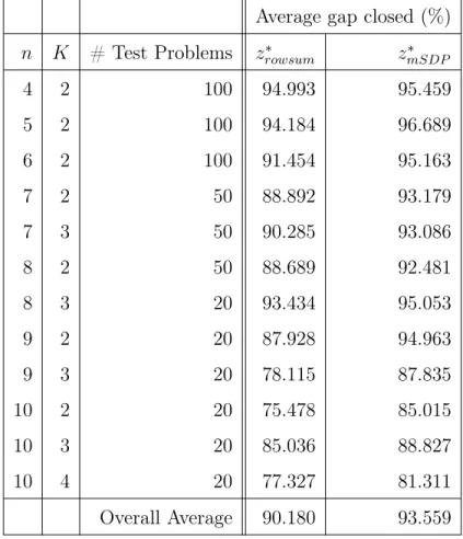
3.2 Test results for randomly generated covariance matrices . . . 76
LIST OF FIGURES
Figure Page
2.1 Spanning trees and induced inequalities for Example 2 . . . 31
2.2 Possible edge labels for two spanning trees of Example 2 . . . 33
2.3 Two spanning trees inducing (2.19) in Example 3 . . . 34
2.4 Label-connected feasible spanning tree for Example 5 . . . 42
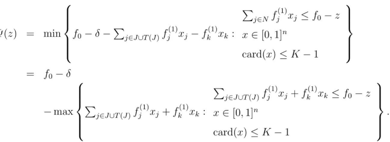
4.1 Ψ(z)and its linear under-estimator for (4.23) . . . 108
ABSTRACT
Kim, Jinhak Ph.D., Purdue University, August 2016. Cardinality constrained opti-mization problems. Major Professor: Mohit Tawarmalani.
In this thesis, we examine optimization problems with a constraint that allows for only a certain number of variables to be nonzero. This constraint, which is called a
cardinality constraint, has received considerable attention in a number of areas such
as machine learning, statistics, computational finance, and operations management. Despite their practical needs, most optimization problems with a cardinality con-straints are hard to solve due to their nonconvexity. We focus on constructing tight convex relaxations to such problems.
We first study linear programs with a cardinality constraint (CCLPs). A procedure that yields cutting planes for any given vector that violates the cardinality constraint is developed. These cutting planes are derived from a disjunctive relaxation of the problem. The separation problem is recast as a network optimization problem where the network is constructed from a simplex tableau of the LP relaxation. We then present a procedure to generate a facet-defining inequality of the disjunctive relaxation using a variant of Prim’s algorithm.
Second, we study an optimization formulation of sparse principal component anal-ysis (sparse PCA). The formulation is a quadratically constrained quadratic problem with a cardinality constraint. The feasible set has a special structure which we call
permutation-invariance. This structure allows us to construct the convex hull of the
feasible set of the model. The convex hull is written through a majorization inequality that can be modeled using a polynomial number variables and linear inequalities. We then show that sparse PCA can be reformulated as a continuous convex maximization problem without a cardinality constraint. In addition, we derive SDP relaxations for
the reformulation. The relaxations are developed based on majorization arguments. The resulting relaxation is provably tighter than the prevalent SDP relaxation pro-posed in [24]. Our preliminary computational results show that our SDP relaxation has gaps 90% smaller than those of the classical SDP relaxation.
Third, we introduce other approaches for CCLPs. We first present a facial dis-junctive reformulation for CCLPs and a finitely-convergent cutting plane algorithm. A generalized reformulation-linearization technique (RLT) is introduced to character-ize the convex hull of the feasible set of CCLPs. As a special subclass of CCLP, we study the cardinality-constrainted knapsack problem (CCKP). We developed families of valid inequalities based on disjunctions for the cardinality constraint.
1. Introduction
Considerable attention has been paid to optimization problems with a constraint that allows only up to a certain number of variables to be nonzero. We call such a constraint a cardinality constraint and any optimization problem containing such a
constraint a cardinality constrained optimization problem (CCOP).
In this thesis, we present relaxation strategies for certain classes of CCOPs using various techniques developed in the fields of mixed-integer linear programming, global optimization, convex and nonconvex optimization.
CCOPs arise in fields as diverse as computational finance, supply chain manage-ment, statistical data analysis, and machine learning. They are used in cardinality-constrained optimal portfolio selection problems in quantitative finance [14, 18, 22,
27, 43, 49, 52, 54]. These problems are variants of the Markowitz mean-variance model where the objective is to minimize a quadratic risk measure under linear constraints along with a restriction that the number of securities chosen for in-vestment is sufficiently small. They also arise in index tracking investment strate-gies [10, 28, 41, 42, 60, 62]. These problems are modeled as time series optimization
models where the objective is to minimize a quadratic tracking error under budget constraints and a restriction that the number of securities selected for investment is small. Facility location problems are classical supply chain management models where a company must decide where to locate facilities. The variant of the problem where at most p warehouses can be opened is known as the p-median problem, and
has been extensively studied in the literature [1,9,21,25,38,47,55]. In statistical data analysis, principal component analysis (PCA) is a well-known technique for dimen-sion reduction. It finds principal components as linear combinations of the original variables. When the coefficients of many variables in these linear combinations are nonzero, the principal components can be hard to interpret. In order to find principal
components that are easier to explain, a cardinality constraint (referred to as a
spar-sity constraint) is sometimes imposed on the original problem. The resulting problem
is known assparse principal component analysis (sparse PCA); see [24,35,46,75].
En-semble pruning [73] and variable selection in multiple regression [12,13] are also often modeled as CCOPs.
Although CCOPs find uses in a variety of applications, they are hard to solve to global optimality. Perhaps the simplest of these problems, which involves optimiz-ing a linear function over the intersection of a continuous knapsack polytope and a cardinality constraint, is already NP-hard [26]. Further, large instances of practical problems are computationally challenging to solve [14,26,54].
For a decision variable x∈Rn,card(x) represents the number of nonzero
compo-nents or the cardinality of x. A cardinality constraint is written as card(x)≤ K for
some positive integerK ∈ {1, . . . , n−1}. In this thesis, we assume thatK >1because
the problem is trivial when K = 1. Therefore, we also assume that n ≥ 3. Various
strategies have been proposed to model cardinality constraints, and to leverage clas-sical MIP branch-and-cut methodologies in the solution of cardinality-constrained problems. When variables x are bounded, auxiliary binary variables can be
intro-duced to model the cardinality constraint. That is, for bounds l, u ∈ Rn such that
liui ≤0 for i= 1, . . . , n, constraints l≤x≤u, card(x)≤K
can be replaced with
l◦z ≤x≤u◦z, 1|z ≤K, z ∈ {0,1}n
where ◦ is the Hardamard product and 1 ∈Rn is the vector whose components are
all equal to one.
When the constraints of the initial problem are linear, such an approach allows the use of branch-and-cut algorithms developed for mixed integer programs (MIPs).
This reformulation also allows for the use of cutting planes derived for cardinality-constrained problems; see [71,72].
In [8] a specialized branch-and-bound algorithm was proposed to solve problems with cardinality constraints where K ∈ {1,2}. These techniques were adapted to
logically constrained linear programs [48], mixed integer quadratic programs [14], and to cardinality-constrained knapsack problems in [26]. Moreover, [26] develops valid inequalities for cardinality constrained knapsack problems (CCKPs) that can be used for cardinality constraint linear programs (CCLPs).
This thesis is organized as follows. In Chapter 2, we develop a procedure that generates cutting planes for CCLPs. For a given LP relaxation of a CCLP and a basic feasible solution, we construct a disjunctive relaxation of the corresponding simplex tableau from which we derive the desired cuts. Specifically, if the given basic feasible solution violates the cardinality constraint, there exists at least K+ 1 basic
variables that correspond to nonzero components of the solution. Then, a disjunctive relaxation of the cardinality requirement can be obtained by imposing a disjunction that forces at least one of those basic variables to be nonpositive. We characterize the closed convex hull of this disjunctive relaxation by obtaining the extreme ray representation of each disjunct and by proving that facet-defining inequalities can be obtained by solving a dual network optimization problem. We further observe that the nontrivial facet-defining inequalities of the relaxation directly relate to a particular class of subgraphs, which we calllabel-connected spanning trees, of a bipartite network
that can be constructed for the the simplex tableau. This procedure generalizes the E&R procedure [56] recently developed in the context of complementarity problems. We then describe a polynomial-time Prim-like algorithm that tightens any given valid inequality of the disjunctive relaxation into a facet-defining inequality. As a special case, we constructively show how the c-max cut, which is a well-known disjunctive cut, can be strengthened to a facet-defining inequality of the convex hull of our disjunctive relaxation when it is not.
Chapter 3 focuses on reformulation and relaxation techniques for an optimization formulation of sparse principal component analysis (sparse PCA). Sparse PCA seeks to find a sparse eigenvector of a given covariance matrix for a centered data matrix. We first provide an extended formulation for the convex hull of sparse PCA by study-ing the dual of the separation problem. The derivation of the convex hull is possible because of a special symmetry structure of the feasible set. More specifically, if a point is in the feasible set, so are all its permutations. We call this property
permutation-invariance. Permutation-invariance enables us to represent the convex hull through
a majorization inequality which can be modeled using a polynomial number of addi-tional variables and linear constraints. The underlying idea is to construct the convex hull over the simplex {x : x1 ≥ · · · ≥ xn ≥ 0} and replicate it onto the remaining
region. By replacing the feasible set of sparse PCA with its convex hull, we relax sparse PCA to a convex maximization problem. We then show that the relaxation is a reformulation of sparse PCA by showing that any optimal solution to the refor-mulated problem that violates the cardinality constraint can always be transformed to a point that satisfies the cardinality constraint and achieves the same objective function value. In addition, we present semidefinite programming (SDP) relaxations for sparse PCA based on majorization arguments on matrix variables. We prove that our SDP relaxations are strictly tighter than a well-known SDP relaxation proposed in [24]. Preliminary computational results obtained for thepitprops dataset and for
randomly generated covariance matrices show that our SDP relaxations have gaps 90% smaller than those of the classical relaxation.
In Chapter 4, we study other approaches to CCLPs. First, we formulate CCLPs as facial disjunctive programs by representing the cardinality constraint in conjunc-tive normal form. That is, card(x) ≤ K is equivalent to enforcing that every
subset of {x1, . . . , xn} of size K + 1 includes at least one zero, or equivalently, V
J∈{1,...,n},|J|=K+1
W
j∈J(xj = 0). The facial structure of the disjunctive set enables us
to apply the finitely-convergent cutting plane algorithm developed by Jeroslow [40]. We then present a generalized reformulation-linearization technique (RLT) to build
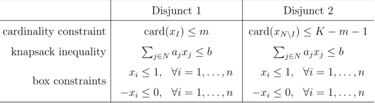
the convex hull of the feasible set of the CCLP. Based on the work of [67], we pro-pose a product factor for generalized RLT that is a ratio of multilinear terms. In the remainder of the chapter, we focus on developing valid inequalities for CCKPs. The derivation is based on the following disjunction that is equivalent to the cardinality constraint card(x)≤K: for a given m ∈ {0, . . . , K},
card(xI)≤m ∨ card(xN\I)≤K−m−1
for any I ⊂ N where xI denotes the |I|-dimensional subvector of x corresponding to
the index setI. This enables us to construct a new valid inequality from a given valid
inequality. We show that the procedure generates a facet-defining inequality from a given facet-defining inequality under certain conditions. We also demonstrate that many valid inequalities proposed in [26] can be derived by our procedure. Finally, we show how to derive some valid inequalities using lifting arguments.
In the last chapter, we summarize the contributions of this dissertation and present directions for future research.
2. On cutting planes for cardinality constrained linear
programming
In this chapter, we derive cutting planes for cardinality-constrained linear programs (CCLPs). These inequalities can be used to separate any basic feasible solution of an LP relaxation of the problem, assuming that this solution violates the cardinality requirement. To derive them, we first relax the given simplex tableau into a disjunc-tive set, expressed in the space of nonbasic variables. We establish that coefficients of valid inequalities for the closed convex hull of this set obey ratios that can be com-puted directly from the simplex tableau. We show that a transportation problem can be used to separate these inequalities. We then give a constructive procedure to gen-erate violated facet-defining inequalities for the closed convex hull of the disjunctive set using a variant of Prim’s algorithm.
2.1 Introduction
In this chapter, we focus on CCOPs, where the optimization problem is linear and refer to them as cardinality-constrained linear programs (CCLPs). A CCLP can be formulated as
maximize c|x+d|y
subject to Ax+By ≤b x, y ≥0
card(x)≤K,
where c, x∈Rp, d, y∈Rq, b ∈Rm, A∈Rm×p, B ∈Rm×q, and K is a fixed positive
constraints. However, for the sake of simplicity in the exposition, we only consider a single cardinality constraint in this research.
We conduct a polyhedral study of CCLPs in the space of original problem vari-ables. In particular, we use information contained in feasible simplex tableaux of LP relaxations of CCLPs to construct strong valid inequalities. Our underlying mo-tivation is that, avoiding the introduction of unnecessary indicator variables will help maintain the original problem structure, and might lead to streamlined solu-tion approaches for these problems. Although we are not aware of previous studies of tableau-based cuts for cardinality-constrained problems, such inequalities have been proposed in the literature in the context of MIPs, quadratic programming, concave programming, and linear complementarity problems [2,7,29,32,37,58,69].
The remainder of this chapter is organized as follows. In Section 2.2, we show that violated cuts for CCLPs can be generated from a disjunctive relaxation of any simplex tableau corresponding to a basic feasible solution violating the cardinality requirement. This disjunctive relaxation has (K + 1) disjuncts, each with a single
nontrivial constraint. We also show that the analysis of the closed convex hull of this set can be performed in the space of nonbasic variables. In Section 2.3, we give a characterization of the closed convex hull based on the extreme ray representation of each disjunct, without the use of disjunctive programming. This characterization relates coefficients of facet-defining inequalities to extreme points of a polyhedron, that we give in closed-form. In Section 2.4, we show that there exists a nonlinear transformation that establishes an isomorphism between the face-lattice of this poly-hedron and that of the dual of a transportation problem. In Section 2.5, we prove that nontrivial facet-defining inequalities of the closed convex hull of the disjunctive set correspond to label-connected spanning trees of the bipartite network associated with the transportation problem. This result allows us to provide, in Section 2.6, a simple explicit constructive procedure for the derivation of nontrivial facet-defining inequalities. It also yields a polynomial time algorithm for the generation of such inequalities, and give a precise characterization of when a commonly used disjunctive
cut, which we refer to as c-max cut, is facet-defining for the disjunctive relaxation. We give concluding remarks in Section 2.7.
2.2 Disjunctive relaxation of a simplex tableau with a cardinality
con-straint
Given an LP relaxation of a CCLP, we next describe an approach to construct cardinality-based cutting planes. We assume that we know a basic feasible solution of this LP relaxation that violates the cardinality constraint, card(x)≤K, together
with an explicit description of the associated simplex tableau. Denoting the basic variables in this tableau by v (indexed by set M), and the nonbasic variables by t
(indexed by setV), we then write the simplex tableau as vl =vl∗− P i∈Vfliti, ∀l ∈ M, vl ≥0, ∀l ∈ M, ti ≥0, ∀i∈ V, (2.1)
where vl∗ ≥ 0 for l ∈ M. Since we have assumed that the current basic solution
(v, t) = (v∗,0)does not satisfy the cardinality constraint, there exists a subsetL ⊆ M
of basic variables such that (i)|L| =K + 1, (ii) variables vl for l ∈ L appear in the
cardinality constraint, and (iii)v∗l >0forl ∈ L. We construct the desired disjunctive
relaxation by (i) relaxing the cardinality constraintcard(x)≤K into the disjunction W
l∈L(vl ≤ 0), which forces one of the K + 1 variables in L to be nonpositive, (ii)
removing the nonnegativity requirements on basic variables, and (iii) omitting the
tableau constraints associated with basic variables vM\L. We therefore study
¯ Q:= (v, t)∈R|L|+|V|: vl =vl∗− P i∈Vfliti, ∀l∈ L, ti ≥0, ∀i∈ V W l∈L(vl ≤0) , (2.2)
where each equality in the above set corresponds to a basic variable in L, and
rep-resents it as an affine function of the nonbasic variables. If a nonbasic variable is a slack variable for a constraint in Ax+By≤b, then an inequality valid forQ¯ can be
written in the space of original problem variables using the defining inequality for the slack variable. We remark that the relaxations applied to the initial simplex tableau in order to obtainQ¯ resemble those made to obtain the corner relaxation of an MIP;
see [31].
Since Q¯ is a finite union of polyhedra, cl conv( ¯Q) is a polyhedron; see Theorem
19.6 in [59] for instance.
Proposition 2.2.1 The set cl conv( ¯Q) is a polyhedron.
A linear inequality is valid for Q¯ if and only if it is valid for cl conv( ¯Q). We
therefore seek to characterize the valid inequalities ofcl conv( ¯Q). We next show that
this can be achieved by studying cl conv(Q) where Q is the projection ofQ¯ onto the
space of nonbasic variablest. Formally, for each l ∈ L, define
Ql := ( t∈R|V|:X i∈V fliti ≥v∗l, ti ≥0, ∀i∈ V ) and setQ:=S
l∈LQl. We assume without loss of generality thatV ={1, . . . , n}. Let h∗(t) = v∗ 0 + −F I
t, where the entry (l, i) of matrix F is fli, as used in the
definition of Q¯ in (2.2). It is clear that h∗(·)is an affine map, and that Q¯ =h∗(Q).
Lemma 1 For i = 1, . . . , p, let Pi ∈ Rn be nonempty polyhedra. Also let h : Rn →
Rm be an affine map. Then
h(cl conv (Sp
i=1Pi)) = cl conv (
Sp
i=1h(Pi)).
Proof It is easy to show that h(Sp
i=1Pi) = Sp i=1h(Pi). Then, cl conv (Sp i=1h(Pi)) = cl conv (h( Sp i=1Pi)) = cl (h(conv (Sp i=1Pi))) ⊇ h(cl conv (Sp i=1Pi)),
where the second equality results from the fact that convex hull operators and affine maps commute, and the last inclusion follows from the continuity ofh. On the other
hand, it is straightforward that
conv (Sp i=1h(Pi)) = conv (h( Sp i=1Pi)) = h(conv (Sp i=1Pi)) ⊆ h(cl conv (Sp i=1Pi)). By Theorem 19.6 in [59], cl conv (Sp
i=1Pi) is a polyhedron and hence its affine
trans-formation is a polyhedron. This implies that h(cl conv (Sp
i=1Pi))is a closed set and
that cl conv (Sp
i=1h(Pi))⊆h(cl conv (
Sp
i=1Pi)).
For the affine function h∗(·)described above, Lemma 1 implies
Proposition 2.2.2 It holds that cl conv( ¯Q) =h∗(cl conv(Q)).
In the remainder of this chapter, we restrict our attention to the study ofcl conv(Q)
since Proposition 2.2.2 shows that this is sufficient to characterize cl conv( ¯Q).
Since we assumed that v∗l > 0 for l ∈ L, we may scale each constraint so that vl∗ = 1. That is, for l∈ L,
Ql= ( t :X i∈V fliti ≥1, ti ≥0,∀i∈ V ) .
For each l ∈ L, define
Il
+ = {i∈ V :fli >0}, I−l = {i∈ V :fli <0}, I0l = {i∈ V :fli = 0}.
Throughout the chapter, we assume without loss of generality thatQl 6=∅for each l ∈ L. In fact, if Ql =∅ for some l ∈ L, then we can simply drop the corresponding
set from the disjunction. It is simple to verify thatQl =∅if and only iffli ≤0for all i∈ V. For this reason, we make the following assumption in the rest of the chapter.
Assumption 1 For each l∈ L, Il
+ 6=∅.
Proposition 2.2.3 Polyhedron Ql is full-dimensional. Further, cl conv(Q) is also
full-dimensional.
Proof By Assumption 1, Il
+ 6=∅. Choosei∈ I+l and consider the point
1 fli + 1 ei+ X k∈V\{i} ek,
where is positive but sufficiently small. This point is in the interior ofQl and hence Qlis full-dimensional. Further, sinceQl⊆Q, thencl conv(Q)is also full-dimensional.
We next argue that there are valid inequalities of cl conv(Q) that can be used
to separate the basic feasible solution associated with the initial simplex tableau (2.1), if this solution violates the cardinality requirement. For instance, consider the inequality
X i∈V
(c−max)iti ≥1 (2.3)
where (c−max)i = max{fli : l ∈ L} for i ∈ V. This inequality, which we refer to
hereafter as c-max cut was introduced in [37] for complementarity problems.
Com-plementarity problems are special instances of cardinality problems requiring that at most one of the variables takes a nonzero value. The c-max cut can be easily seen to be valid for cl conv(Q) because P
i∈V(c−max)iti ≥ P
i∈Vfliti ≥ 1 for all t ∈ Ql
and l ∈ L, i.e., it is valid for each disjunct Ql. Moreover, it separates the closed
convex hull from t = 0 because this point violates (2.3). For the particular case
when |L| = 2, it is shown in [56] that the c-max cut is not always facet-defining for cl conv(Q) and is not sufficient to provide a complete description of the nontrivial
inequalities of cl conv(Q). In this chapter, we provide a complete description of the
nontrivial facet-defining inequalities of cl conv(Q). We show that all nontrivial
facet-defining inequalities of cl conv(Q) cut off the current basic feasible solution of (2.1),
2.3 A characterization of cl conv(Q)
In this section, we provide a characterization of the facet-defining inequalities of
cl conv(Q). Recall that Minkowski-Weyl’s theorem, see Theorem 7.13 in [36] for
in-stance, establishes that a polyhedron can be represented in two forms, either using its vertices and extreme rays or as a finite intersection of half-spaces. Following [74], we refer to the former representation as a V-polyhedron, and to the latter as a H
-polyhedron. Through the rest of the chapter, we alternate between these
representa-tions when studying cl conv(Q). We also find it more convenient to study a certain
homogenization of Q. We show in Proposition 2.3.4 that studying this
homogeniza-tion is without loss of generality.
Let V0 :=V ∪ {0}. Define Q0l to be the homogenization of Ql obtained as
Q0l := ( t := (t1, . . . , tn, t0)∈R|V0|: X i∈V fliti ≥t0, t≥0 ) .
After defining fl0 :=−1 and fl:= (fl1, . . . , fln, fl0)|, we can rewrite Q0l as
Q0l =t∈R|V0|:f|
lt≥0, t≥0 .
We refer to fl|t ≥ 0 as the nontrivial constraint of disjunct l. It is clear that Q0l is
a polyhedral cone. Referring to S
l∈LQ0l as Q0, it is also clear that cl conv(Q0) is a
cone. We next describe how these cones relate to the sets we originally introduced. For a nonempty convex set C, we define K(C) :={λ(d,1) : d∈C, λ >0}.
Proposition 2.3.1 It holds that 1. Q0
l = cl(K(Ql)).
2. cl conv(Q0) = cl(K(cl conv(Q))).
Proof First, we prove 1. We refer to K(Ql) as K. To show cl(K) ⊆ Q0l, consider λ(d,1) ∈ K for some λ > 0 and d ∈ Ql. Then, Pi∈Vflidi ≥ 1. Since λ(d,1) ≥ 0
and fl|λ(d,1) = λ(P
i∈Vflidi −1) ≥ 0, then λ(d,1) ∈ Q0l. Since Q
0
cl(K) ⊆ Q0
l. To show Q0l ⊆ cl(K), consider (d, d0) ∈ Q0l. If d0 > 0, then d/d0 ∈ Ql
and hence (d, d0) = d0(d/d0,1) ∈ K. Now, assume d0 = 0. Then, Pi∈Vflidi ≥ 0.
Since Ql 6= ∅ by Assumption 1, we may select d0 ∈ Ql. Then, for any µ > 0, d0 +µd ∈ Ql because Pi∈Vfli(d0 +µd)i = Pi∈Vflid0i +µ
P
i∈Vflidi ≥ 1. Hence
(1/µ)(d0 +µd,1) ∈ K. Observe that limµ→∞(1/µ)(d0 +µd,1) = (d,0). Therefore,
(d, d0) = (d,0)∈cl(K).
We next prove 2. Clearly, cl conv(Q0)⊇ K(cl conv(Q)) because K(cl conv(Q))⊆ cl conv(K(Q)) ⊆ cl conv(Q0), where the first inclusion holds because cl conv(Q) ⊆
cl conv(K(Q)) and cl conv(K(Q)) is a cone, and the second inclusion is because
K(Q) =S
l∈LK(Ql)⊆Sl∈LQ0l =Q0. For the reverse inclusion, observe that: Q0 =[
l∈L
Q0l =[
l∈L
cl(K(Ql))⊆cl(Kcl conv(Q))),
where the first equality is by definition of Q0, the second by Part 1, and the first
inclusion is because Ql ⊆ cl conv(Q). Since cl(K(cl conv(Q))) is closed and convex,
cl conv(Q0)⊆cl(K(cl conv(Q))).
Propositions 2.2.3 and 2.3.1 directly yield
Corollary 1 Polyhedron cl conv(Q0) is full-dimensional.
In Proposition 2.3.2, we presentV-polyhedron representations ofQ0
l and Ql. This
result allows us to build V-polyhedron representations ofcl conv(Q0) and cl conv(Q)
in Corollary 2. Proposition 2.3.2 Define R0l = {fliej−fljei ∈R|V0| :i∈ I+l, j ∈ I l −∪ {0}} ∪ {ek ∈R|V0|:k∈ I+l ∪ I l 0}, Vl = 1 fli ei ∈R|V| :i∈ I+l , Rl = {fliej−fljei ∈R|V| :i∈ I+l, j ∈ I l −} ∪ {ek ∈R|V|:k ∈ I+l ∪ I l 0}.
Then Q0l = cone(Rl0)and Ql = conv (Vl) + cone(Rl). Further all the given points and
Proof We first show that Q0
l = cone(R0l). Since Q0l is a cone in the nonnegative
orthant, it is pointed. This implies that all the points in the cone can be written as a conic combination of its extreme rays. Let r be a ray of Q0
l. Then, r is extreme
if and only if it belongs to the intersection of n =|V0| −1 independent hyperplanes
among {t ∈ R|V0| : f|
lt = 0} and {t ∈ R |V0| : t
k = 0}, for k ∈ V0. First, for each
i ∈ V0, suppose that these n hyperplanes are {t : tk = 0} for k 6= i. Then rk = 0
for all k 6= i and hence r = ρei with ρ > 0. In order to be a ray, this vector must
satisfy fl|r ≥ 0, i.e., i must be chosen in Il
+ ∪ I0l . Next, suppose that these n
hyperplanes are {t ∈ R|V0| : f|
lt = 0} and {t ∈ R
|V0| : t
k = 0} for k 6= i, j for
some i, j ∈ V0. Then the face defined by the intersection of these hyperplanes is
F := {t ∈ R|V0| : f
liti+fljtj = 0, t ≥ 0, tk = 0,∀k 6= i, j}. In order for r to be a
ray, F 6= {0} and hence fliflj ≤ 0. By independence, fli 6= 0 or flj 6= 0. If fli = 0
or flj = 0 then we have that r = ek for some k ∈ I0l. Now assume that fliflj < 0.
Without loss of generality, assume that fli > 0 and flj < 0. Then, r =fliej −fljei
where i ∈ Il
+ and j ∈ I−l ∪ {0}. We conclude that Rl0 is precisely the collection of
extreme rays of Q0l, and thereforeQ0l = cone(Rl0).
We next prove that Ql = conv (Vl) + cone(Rl). By Proposition 2.3.1 and by
Lemma 5.41 of [36], we have that
Ql = conv(Vl0) + cone(R 0 l)
where Vl0 is the set of vectors tt
0 in R
|V| obtained from rays (t, t
0) of Q0l whose
com-ponent t0 is nonzero, and R0l is the set of vectors t in R
|V| obtained from rays (t, t
0)
of Q0
l where t0 = 0. Thus, Vl0 = Vl and R0l =Rl. Extremality follows directly from
the extremality of rays in R0
l.
The result of Proposition 2.3.2 yields aV-polyhedron representation for the closed
convex hull of the union of the associated disjuncts.
Corollary 2 The V-polyhedron representations of cl conv(Q0) and cl conv(Q) are
cl conv(Q0) = cone(R0),
where R0 :=S l∈LR0l, V := S l∈LVl, and R := S l∈LRl.
We now seek to better understand the coefficient vectors β ∈R|V| and β0 ∈ R|V0|
that give rise to strong valid inequalities of cl conv(Q) and cl conv(Q0), respectively.
We show next that β and β0 are closely related.
Proposition 2.3.3 Inequality
X i∈V
βiti ≥γ (2.4)
is valid for cl conv(Q) if and only if inequality
X i∈V
βiti ≥γt0 (2.5)
is valid for cl conv(Q0).
Proof For the direct implication, suppose that (2.4) is valid for cl conv(Q). Take
any (d, d0) ∈ K(cl conv(Q)). By definition, (d, d0) = d0(dd0,1) where d0 > 0 and
d
d0 ∈ cl conv(Q). It follows that
P
i∈Vβidi ≥ γd0. This shows that (2.5) is valid for
K(cl conv(Q)), and therefore, by Proposition 2.3.1, for cl conv(Q0). For the reverse
implication, suppose now that (2.5) is valid for cl conv(Q0). Take any d ∈ Q. Then (d,1)∈Q0. Since (2.5) is valid for cl conv(Q0), thenP
i∈Vβidi ≥γ. This shows that
(2.4) is valid for cl conv(Q).
The following result shows that characterizing the facets of cl conv(Q0) is
equiva-lent to characterizing the facets of cl conv(Q).
Proposition 2.3.4 Inequality (2.4) is facet-defining for cl conv(Q) if and only if in-equality (2.5) is facet-defining for cl conv(Q0) and is not a scalar multiple of t
0 ≥0.
Proof The fact that validity is preserved is shown in Proposition 2.3.3. Suppose
now that (2.4) is facet-defining for cl conv(Q). Then there exist n = |V| affinely
independent points w1, . . . , wn of cl conv(Q) that satisfy (2.4) at equality. Points (wj,1) belong to cl conv(Q0) for all j ∈ V and satisfy (2.5) at equality. Since {wj :
j ∈ V} are affinely independent, {(wj,1) : j ∈ V} are linearly independent. This
proves that (2.5) is facet-defining for cl conv(Q0). Clearly, (2.5) is not t0 ≥ 0 as
otherwise (2.4) would be 0|t ≥ −1, which is not facet-defining for cl conv(Q).
Conversely, suppose that (2.5) is facet-defining for cl conv(Q0). Sincecl conv(Q0)
is a full-dimensional polyhedral cone, there exist nlinearly independent extreme rays
(rj, rj0) of cl conv(Q0) that satisfy (2.5) at equality. Suppose rj0 = 0 for all j ∈ V.
Observe that {rj : j ∈ V} are linearly independent and β|rj = 0 for allj ∈ V. This
shows thatβ = 0. However, this is not possible as (2.5) would then correspond to the
face of cl conv(Q0) induced by t
0 ≥ 0. Therefore, there must exist j ∈ V such that
rj0 6= 0. Define I1 = {j0 ∈ V : rj 0 0 6= 0}(6= ∅) and I2 = {j0 ∈ V : rj 0 0 = 0}. Then, for j ∈ I1, β|r j rj0 = 1 rj0 β|rj = γ. Further, for k ∈ I
2, β|rk = 0. Fix j0 ∈ I1, and consider
the sets of points
rj rj0 :j ∈I1 ∪ rj0 rj0 0 +rk :k ∈I2 .
It is clear that these points satisfy (2.4) at equality and that they belong tocl conv(Q)
by Proposition 2.3.1. It remains to prove that they are affinely independent, which can be established easily because the linear independence of vectors
rj rj0 − rj0 rj0 0 :j ∈I1\ {j0} ∪ rk :k ∈I2
follows from the assumed independence of{(rj, r0), j ∈ V}. Therefore, (2.4) is
facet-defining for cl conv(Q).
In the remainder of this chapter, we prefer to study cl conv(Q0) because, being
homogeneous, it allows for a unified treatment of the extreme points and extreme rays of Q, and thus permits a more streamlined presentation.
We are now ready to further investigate the structure of coefficient vectors associ-ated with facet-defining inequalities (2.5) of cl conv(Q0). In particular, we will show
in Proposition 2.3.6 that, except for some simple inequalities we describe next, most facet-defining inequalities are such that γ >0.
For i ∈ V0, we refer to the inequalities ti ≥ 0 of cl conv(Q0) as trivial. For
notational convenience, we redefineIl
−:=I−l ∪ {0}. HenceI+l,I−l , andI0l exclusively
partition V0. We also define
I+ ={i∈ V0 :fli >0for some l ∈ L} = S l∈LI+l , I− ={i∈ V0 :fli <0for all l ∈ L} = T l∈LI−l , I0 =V0 \(I+∪ I−).
It is clear that 0∈ I− and it follows from Assumption 1 that I+ 6= ∅. We establish
next that trivial inequalities are typically facet-defining forcl conv(Q0).
Proposition 2.3.5 Trivial inequality ti ≥ 0 is facet-defining for cl conv(Q0) if and
only if
1. i∈ I−∪ I0, or
2. i∈ I+ and |I+| ≥2.
Proof Inequalityti ≥0is clearly valid forcl conv(Q0). Assume first thati∈ I−∪I0.
Since I+6=∅, there exists j ∈ I+ and l ∈ L such that flj >0. Consider the point
X k∈V0\{i,j} ek+ 1−P k∈V0\{i,j}flk flj ej (2.6)
for positive and sufficiently small. This point is in the relative interior of Q0
l ∩ {t∈
R|V0|:t
i = 0}. Hence, it is in the relative interior ofcl conv(Q0)∩ {t∈R|V0|:ti = 0}.
It follows that ti ≥ 0 is facet-defining for cl conv(Q0). Next, assume that i ∈ I+.
If |I+| ≥ 2, there exists j ∈ I+\ {i} and l ∈ L such that flj > 0. Then, (2.6) is
an interior point of Q0
l ∩ {t ∈ R |V0| : t
i = 0} and hence ti ≥ 0 is facet-defining for
cl conv(Q0). Suppose I
+ = {i} and j ∈ I−. Then, for each l ∈ L, every point in Q0
l ∩ {t ∈ R |V0| : t
i = 0} satisfies tj = 0. It follows that ti ≥ 0 defines a face of
cl conv(Q0)of dimension at least two less than that of cl conv(Q0), showing that this
Proposition 2.3.5 shows that trivial inequalities ti ≥ 0 are facet-defining unless i∈ I+and |I+|= 1. In the remainder of this chapter, we considerβ to be a vector in R|V0|. We show next that the sign of the entries of coefficient vectors β for nontrivial
facet-defining inequalities ofcl conv(Q0)can be deduced directly from the setsI+,I−,
and I0.
Proposition 2.3.6 Let
X i∈V0
βiti ≥0. (2.7)
be a nontrivial facet-defining inequality for cl conv(Q0). Then
1. βi ≥ −max{fli :l∈ L}β0 for i∈ I+,
2. βj <0 for j ∈ I−,
3. βk= 0 if max{flk :l ∈ L}= 0.
In particular, βi >0 for i∈ I+.
Proof Consider a nontrivial facet-defining inequality (2.7). Observe that βi ≥0for i∈ I+∪ I0 because ei is a ray ofQ0.
We first prove 1. Choose j0 ∈ I− with βj0 <0. Such a j0 exists because otherwise,
(2.7) is implied by trivial inequalities. Leti∈ Il
+ for some l∈ L. Sincefliej0 −flj0ei
is a ray for cl conv(Q0), it follows that β
i ≥max{fli :l ∈ L} βj0
flj0 >0. Remember now
that 0∈ I−. Ifβ0 <0, Part 1 follows easily since fl0 =−1. Ifβ0 = 0, Part 1 simply
states that βi ≥0while the inequality just proven for j0 is stronger.
We now prove 2 and 3. Consider j ∈ I− ∪ I0. There exists an extreme ray r
of cl conv(Q0) such that β|r = 0 and r
j > 0 because otherwise, (2.7) is a trivial
inequality. Proposition 2.3.2 shows that this ray can be of one of two forms. First assume that r =fliej−fljei for some l ∈ L and i∈ I+l. As shown above, βi >0. It
follows from β|r= 0 that βj <0. This shows Part 2 when j ∈ I− and shows that it
βj ≥ 0. Now, consider j ∈ I0. We must have that r = ej. This shows that βj = 0
proving Part 3.
Example 1 Consider the set Q0 with disjuncts defined by the constraints 5t1 −3t2 +0t3 +1t4 −5t5 −t0 ≥0 3t1 −1t2 +2t3 −3t4 −3t5 −t0 ≥0 4t1 −6t2 +4t3 −2t4 +0t5 −t0 ≥0 2t1 −2t2 −2t3 +0t4 −2t5 −t0 ≥0. (2.8) Then I+ ={1,3,4}, I− ={2,0}, and I0 ={5}.
We use PORTA [19, 20] to obtain the extreme rays of each disjunct independently. We then run PORTA again based on this collection of extreme rays to obtain all facet-defining inequalities ofcl conv(Q0). The resulting nontrivial facet-defining inequalities
are
5t1 −53t2 +4t3 +t4 +0t5 −t0 ≥0 9t1 −3t2 +6t3 +t4 +0t5 −t0 ≥0 6t1 −2t2 +4t3 +t4 +0t5 −t0 ≥0.
(2.9)
We observe that, as argued in Proposition 2.3.6, βi >0 for i∈ I+, βi <0 for i∈ I−
and β5 = 0 in all nontrivial facet-defining inequalities (2.9).
Proposition 2.3.6 shows that nontrivial facet-defining inequalities of cl conv(Q0)
are such that βk is zero for each index k for which the tableau coefficients satisfy flk ≤0for all l ∈ Land fl0k = 0 for some l0 ∈ L. Then, it is clear that cl conv(Q) = {t = (t−k, tk) : t−k ∈ cl conv(Q−k), tk ∈ R+} where t−k is the vector obtained by
dropping component tk from t and Q−k := projt−k(Q). Thus, it is sufficient to study cl conv(Q−k). For this reason, we make the following assumption in the remainder of
the chapter.
With Assumption 2, it follows that I+ and I− exclusively partition V0.
We next derive anH-polyhedron representation of cl conv(Q0). We obtain the
lin-ear inequalities of this representation by considering the dual cone of itsV-polyhedron
representation, which was obtained in Corollary 2. For a given cone C ⊆Rn, we
de-note the dual cone of C by C∗. Recall that C∗ ={y ∈ Rn : y|x ≥ 0, ∀x ∈ C}. As
we established in Corollary 2 that cl conv(Q0) = cone(R0)where R0 :=S
l∈LR0l, it is
easy to see that β|t ≥ 0 is a valid inequality for cl conv(Q0) if and only if β|r ≥ 0
for all r ∈ R0. Therefore, the coefficient vectors of valid inequalities for cl conv(Q0)
belong to B1 = β ∈R|V0|: fliβj −fljβi ≥0, ∀(i, j)∈ I l +× I−l, l ∈ L βk ≥0, ∀k∈ I+l ∪ I0l, l ∈ L , (2.10)
where we use B1 as a shorthand notation for [cl conv(Q0)]∗.
Among the facet-defining inequalities of cl conv(Q0), trivial inequalities are not
useful in practice, since they do not cut off the basic solution associated with simplex tableau (2.1). We therefore concentrate on nontrivial facet-defining inequalities of
cl conv(Q0), which have β
0 <0 as shown in Proposition 2.3.6. Therefore, by scaling
if necessary, we may assume that β0 = −1. For this reason, we focus our ensuing
study on B2 := B1 ∩ {β ∈ R|V0| : β0 = −1}, and show that the description of this
polyhedron requires fewer constraints than those given in (2.10).
Proposition 2.3.7 For (i, j)∈ I+× I−, define wij = min −flj fli :fli >0, l∈ L . (2.11) Then B2 = β ∈R|V0|: βj +wijβi ≥0, ∀(i, j)∈ I+× I− β0 =−1 . (2.12)
Proof Just as in the proof of Proposition 2.3.6, whenβ0 <0, the inequalitiesβk≥0
fork ∈ Il
+∪ I0l do not supportB1 and can therefore be dropped. Now, for anyi∈ I+l
and j ∈ Il
−, βi ≥ ffli
ljβj. This inequality is redundant if j ∈ I+ because, as argued
above, βi >0. Therefore, j ∈ I−. Maximizing ffli
It is easy to see that the coefficients β ∈ B2 are sign-constrained. Therefore, B2
has no lines. Because B2 does not have a line, it has at least one extreme point; see
Corollary 18.5.3 in [59]. We mention that B2 does also have rays, including vectors
ei for i∈ I+∪ I−\{0}.
We next show that there is a one-to-one correspondence between the nontrivial facet-defining inequalities of cl conv(Q0) and the extreme points ofB2.
Theorem 2.3.1 Any inequalityβ|t≥0withβ
0 =−1is facet-defining forcl conv(Q0)
if and only if β is an extreme point of B2.
Proof For a facet-defining inequality, β|t≥0 of cl conv(Q0), β is an extreme point
of B2 because of the n linearly independent tight constraints β|rj = 0, one for each
tight linearly independent extreme ray rj of cl conv(Q0) and the equality constraint
β0 =−1. For the reverse inclusion, the tight constraints, besides β0 =−1, each yield
a linearly independent extreme ray tight for the inequality.
Extreme rays ofB2also lead to valid inequalities forcl conv(Q0). In fact, consider a
solutionβand an extreme rayρofB2. Clearly,ρ0 = 0. For allτ ≥0,β+τ ρ∈B2, and
therefore the inequality (β+τ ρ)|t ≥0 is valid for cl conv(Q0). Dividing throughout
by τ and letting τ → ∞, we then conclude that ρ|t ≥ 0, an inequality with ρ
0 = 0,
is valid for cl conv(Q0). If this inequality is facet-defining for cl conv(Q0), then it
must be one of the trivial ones. However, extreme rays, unlike extreme points, do not necessarily yield facet-defining inequalities for cl conv(Q0). We next illustrate these
observations, together with the statement of Theorem 2.3.1.
Example 1 (continued) For the set Q0 with disjuncts defined by (2.8) and where
variable t5 has been removed, we compute that w12 := min
3 5, 1 3, 6 4, 2 2 = 1 3, w10 :=
min15,13,14,12 = 15, w32 := min 1 2, 6 4 = 1 2, w30 := min 1 2, 1 4 = 1 4, w42 := 3, and
w40:= 1. It then follows from Proposition 2.3.7 that
B2 = (β1, β2, β3, β4, β0)∈R5 : β2 + 13β1 ≥ 0 β0 + 15β1 ≥ 0 β2 + 12β3 ≥ 0 β0 + 14β3 ≥ 0 β2 + 3β4 ≥ 0 β0 + β4 ≥ 0 β0 = −1 .
Coefficient vectors of all facet-defining inequalities of cl conv(Q0)that cut off the solu-tion(0,0,0,0,1)belong toB2. For instance, the coefficient vectorβ = (5,−53,4,1,−1)
belongs to B2. Further, it satisfies the following system of linearly independent
equa-tions β2+13β1 = 0, β0+15β1 = 0, β0+14β3 = 0, β0+β4 = 0, and β0 =−1. Since the
system has a unique solution, β is an extreme point of B2. This extreme point is the
coefficient vector of the first facet-defining inequality of (2.9) (where we have omitted
the coefficient β5 since I0 = {5}). It can also be verified that (3,−1,2,13,0) is an
extreme ray ofB2. It corresponds to the valid inequality3t1−t2+ 2t3+13t4 ≥0, which
is not facet-defining for cl conv(Q0) since it can be obtained as a conic combination
of the second facet-defining inequality of (2.9) and t0 ≥0 with equal weights of 13.
2.4 Dual network formulation of B2
In this section, we present a nonlinear transformation that maps (a subset of) the polyhedronB2to the feasible region of the dual of a transportation problem. We show
that this transformation preserves the face-lattice of B2 (see below for a definition.)
We use these results in Section 2.5 to establish a correspondence between the extreme points of B2, i.e., the nontrivial facet-defining inequalities ofcl conv(Q0), and certain
We have shown in Proposition 2.3.6 that if β is an extreme point of B2, βi > 0
for all i∈ I+ and βj <0 for all j ∈ I−. Define A={β ∈ R|V0| :βi >0, βj <0,∀i∈ I+,∀j ∈ I−}. Observe that, for any β ∈B2∩A and for (i, j)∈ I+× I−,
βj +wijβi ≥0 ⇐⇒
−βj βi
≤wij ⇐⇒ log(−βj)−log(βi)≤log(wij).
All the logarithms computed above are well-defined under the conditions ofA. Define T :A→R|V0| by [T(β)]k:= log|βk|= log(βk) if k ∈ I+ log(−βk) if k ∈ I−.
Its inverse transformation T−1 is
[T−1(δ)]k = eδk if k ∈ I + −eδk if k ∈ I −.
After introducing the new variables δi = log(βi), for i ∈ I+ and δj = log(−βj),
for j ∈ I−, and the constants cij = log(wij), for (i, j)∈ I+× I−, we define
D1 := δ∈R|V0| :δ j −δi ≤cij,∀(i, j)∈ I+× I− , D2 := δ∈R|V0| :δ j −δi ≤cij, δ0 = 0,∀(i, j)∈ I+× I− .
Proposition 2.4.1 It holds that T(B2∩A) =D2.
It is clear that for β ∈B2∩A and δ =T(β)∈D2,
βj+wijβi = 0 ⇐⇒ δj −δi =cij, (2.13) βj +wijβi ≤0 ⇐⇒ δj −δi ≤cij. (2.14)
LetH(E)be the subgraph of the complete bipartite graphG:= (I+,I−)with edge
setE ⊆ I+× I−. Let P, Q∈R|I+|×|I−| be two matrices. We create the |E| ×(n+ 1)
matrix M(H(E), P, Q) by fixing an ordering of the edges of E (say lexicographical)
and by assigning the row of M(H(E), P, Q) corresponding to edge {i, j} ∈ E to be
Lemma 2 Assume that H(E) is a subforest of G. Assume also that Pij 6= 0 and Qij 6= 0 for all {i, j} ∈E. Then M(H(E), P, Q) has full rank.
Proof Suppose H(E) is a subforest ofG. Since|E|< n+ 1, we only need to prove
independence of the rows ofM(H(E), P, Q). For a positive integerk= 1, . . . ,|E| −1,
observe that the (k + 1)th row of M(H(E), P, Q) introduces a new nonzero entry, which was zero in the first k rows because H(E) does not contain a cycle, Pij 6= 0
and Qij 6= 0. This shows that the rows of M(H(E), P, Q) are independent.
Define Jto be the |I+| × |I−|matrix of ones and Wto be the |I+| × |I−| matrix
whose (i, j)entry is wij. For any E ⊆ I+× I− such that H(E) is a forest, Lemma 2
shows that both matrices M(H(E),J,−J)and M(H(E),J,W) have full rank.
Proposition 2.4.2 Let H(E) be a subgraph of G with n =|V0| −1 edges such that
rank(M(H(E),J,W)) = n and M(H(E),J,W)β = 0 for some β ∈B2. Then H(E)
is a tree of G.
Proof Assume by contradiction thatH(E)has a cycleC, and letβC be the
compo-nents ofβassociated with nodes ofC. LetM0be then×nsubmatrix ofM(H(E),J,W)
associated with cycleC. Then it is easy to verify thatM0is nonsingular andM0βC = 0
which implies that βC = 0. Since G is bipartite, C contains a node k ∈ I+, and so
βk = 0. Because β ∈B2, it satisfies β0+wk0βk ≥0, which implies that β0 ≥0. This
is a contradiction to the fact thatβ0 =−1. SinceH(E)has n edges,n+ 1 nodes and
no cycle, it is a tree.
A finite partially ordered set (S,≤), or poset, is the association of a finite setS with
a relation “≤” which is (i) reflexive: x ≤ x for all x ∈ S, (ii) transitive: x ≤ y and y ≤ z imply x ≤ z, and (iii) antisymmetric: x ≤ y and y ≤ x imply x = y. The
face-lattice of a polyhedronP is the poset of its faces, partially ordered by inclusion.
We say that two posets (S,≤) and (S0,) are isomorphic if there is a bijection T(·)
from S to S0 such that s1 ≤ s2 if and only if T(s1) T(s2). Moreover, we say two
Proposition 2.4.3 Polyhedra D2 and B2 are isomorphic.
Proof Given a polyhedron P ⊆ Rn, we define F(P) to be the set of faces of P.
Given E ⊆ I+× I−, we define
B2|E = {β ∈B2|βj +wijβi = 0,∀(i, j)∈E} D2|E = {δ ∈D2|δj−δi =cij,∀(i, j)∈E}.
Clearly, B2|E and D2|E are (possibly empty) faces of B2 and D2, respectively.
Given a nonempty face F of B2, we denote byE(F) the largest subset E ⊆ I+× I−
such that F = B2|E. In particular, for every point β∗ in the relative interior of F, βj∗+wijβi∗ < 0 for (i, j)∈ (I+× I−)\E(F). Similarly, given a nonempty face F0 of D2, we denote by E0(F0) the largest subset E0 ⊆ I+× I− such that F0 =D2|E0. For
every pointδ∗ in the relative interior of F0, δj−δi < cij for (i, j)∈(I+× I−)\E0(F0).
Next, we define ϕ : F(B2) 7→ F(D2) to be such that ϕ(F) = D2|E(F) for any
nonempty faceF ∈ F(B2)andϕ(∅) =∅. We show thatϕis a bijection by
construct-ing an inverse to ϕ. Define ψ : F(D2) 7→ F(B2) to be such that ψ(F0) = B2|E0(F0)
for any nonempty face F0 ∈ F(D2) and ψ(∅) =∅. First, we argue that if F ∈ F(B2)
and F0 = ϕ(F), then E(F) = E0(F0). Consider a point β¯ in the relative interior of F and an extreme point β˜ of that face. The line segment [ ¯β,β˜) is in the relative
interior of F; see Theorem 6.1 of [59]. Further, there exists a point β on this line
segment, sufficiently close to β˜, that belongs to A. Define δ= T(β). It follows from
(2.13) and (2.14) thatδ belongs to the relative interior ofF0 and thatE(F) =E0(F0).
Similarly, if F0 ∈ F(D2) and F00 = ψ(F0), then E0(F0) = E(F00). Second, we argue
that for each F ∈ F(B2), ψ(ϕ(F)) = F. The result is clear when F = ∅. When
F 6=∅, define F0 =ϕ(F) and F00 =ψ(F0). It follows from the above discussion that E(F) =E0(F0) = E(F00) ThereforeF00 =B2|E(F00) =B2|E(F) =F.
To conclude the proof, consider two faces F1 and F2 ofF(B2) such thatF1 ⊆F2.
Define F10 =ϕ(F1) and F20 = ϕ(F2). Since F1 ⊆ F2, then E(F1) ⊇ E(F2). It follows
from the above discussion that E0(F10) ⊇ E0(F20), showing that ϕ(F1) = F10 ⊆ F20 =
It is shown in Theorem 10.1 of [17] that two isomorphic polytopes have the same dimension, and that faces matched through the bijection T(·) have identical
dimen-sions. The proof idea extends to our setting.
The proof of Proposition 2.4.3 shows that there is a one-to-one correspondence between the faces of dimension one of B2 and D2. We obtain
Corollary 3 If u is an extreme point of D2 then T−1(u) is an extreme point of B2.
Conversely, if v is an extreme point of B2 then T(v) is an extreme point of D2.
Extreme points ofD2 can be exposed as unique optimal solutions to certain linear
programs (LPs) over D2, or equivalently can be obtained from optimal solutions of
certain LPs overD1. In order for such LPs to have an optimal extreme point solution,
the objective coefficient vector should be chosen in the polar cone of the recession cone of the feasible set. The recession cones of D1 and D2 are
rec(D1) = {δ∈R|V0| :δj −δi ≤0,∀(i, j)∈ I+× I−},
rec(D2) = {δ∈R|V0| :δj −δi ≤0, δ0 = 0,∀(i, j)∈ I+× I−}.
We next derive a V-polyhedron description ofrec(D1)and rec(D2). In this result,
we let1=P
k∈V0ek. For a set of vectorsV, we definelin(V)to be the linear subspace
generated by V. For notational convenience, we write lin(v) = lin({v}) for a vector
v.
Proposition 2.4.4
1. Let R2 = {ei : i ∈ I+} ∪ {−ej : j ∈ I−\ {0}} ∪ {1−e0}. Then rec(D2) = cone(R2).
2. Let R1 ={ei :i∈ I+} ∪ {−ej :j ∈ I−}. Then rec(D1) = cone(R1) + lin(1).
Proof Assume that δ ∈ rec(D2). Let a = min{δi : i ∈ I+} and b = max{δj : j ∈ I−}. Then, b ≥ δ0 = 0. Furthermore, δj ≤ b ≤ a ≤ δi, for i ∈ I+ and j ∈ I−. We
can then write
δ=b(1−e0) + X j∈I−\{0} (b−δj)(−ej) + X i∈I+ (δi−b)ei,
which shows that rec(D2)⊆cone(R2). Observe next that R2 ⊆rec(D2) since the
elements of R2 are rays of D2. Therefore cone(R2) ⊆ rec(D2), proving 1. We next
show that rec(D1) = rec(D2) + lin(1), which will prove 2 since 1−e0 ∈ −e0+ lin(1).
To prove the forward inclusion (⊆), consider δ0 inrec(D1). Thenδ0−δ001 belongs to
rec(D2). To prove the reverse inclusion (⊇), consider δ0 in rec(D2) and t ∈ R. It is
clear that δ0 +t1∈rec(D1).
By definition of polar cone,
(rec(D1))o := {y :y|x≤0, x∈rec(D1)} = {y :y|x≤0, x∈R1∪ {−1,1}} = y : y|e i ≤0, ∀i∈ I+ y|(−e j)≤0, ∀j ∈ I− y|1= 0 = y : yi ≤0, ∀i∈ I+ yj ≥0, ∀j ∈ I− P k∈V0yk = 0 .
Similar to B2, it is simple to verify that D2 does not contain lines, and therefore
has at least one extreme point. We next show that each extreme point of D2 can be
derived from an optimal solution of an LP overD1by setting an appropriate objective
vector y inri (rec(D1)o). Define s:=−yI+ and d:=yI−. The desired LP is
max −X i∈I+ siδi+ X j∈I− djδj s.t. δj −δi ≤cij, ∀(i, j)∈ I+× I−. (2.15)
Its dual is the transportation problem:
min X i∈I+ X j∈I− cijxij s.t. X j∈I− xij =si, ∀i∈ I+, X i∈I+ xij =dj, ∀j ∈ I−, (2.16) xij ≥0 ∀(i, j)∈ I+× I−.
We next argue that both primal (2.16) and dual (2.15) problems are feasible, thereby showing that optimal primal and dual solutions exist. The primal problem (2.16) is feasible because P
j∈I−dj = P
i∈I+si. The c-max cut shows that the dual
problem (2.16) is feasible. In fact, let c−max be the coefficient vector of the c-max
cut. This vector is in B2. Furthermore, (c−max)i >0 for i ∈ I+ and (c−max)j <0
for j ∈ I−. Therefore, (c−max) ∈ B2∩A. It follows that T(c−max) ∈ D2 ⊆ D1.
The fact that D1 is nonempty also follows from Proposition 2.4.3.
Proposition 2.4.4 shows that D1 has a lineality. It follows that the faces of D1
of smallest dimension are edges. Because (2.15) has an optimal solution, it must therefore be that it has an edge of optimal solutions. Let δ0 be a solution on this
edge. There are n active constraints of D1 atδ0. Now defineδ∗ =δ0−δ001. Then,
−X i∈I+ siδ∗i + X j∈I− djδj∗ = − X i∈I+ si(δi0−δ0) + X j∈I− dj(δj0 −δ0) = −X i∈I+ siδi0+ X j∈I− djδj0 +δ0( X i∈I+ si− X j∈I− dj) = −X i∈I+ siδi0+ X j∈I− djδj0.
Hence δ∗ has the same objective function value as δ0. Moreover, δ∗ satisfies all
the constraints in (2.15) because δ∗j −δ∗i = (δj0 −δ00)−(δ0i−δ00) = δj0 −δi0 ≤ cij for
all (i, j) ∈ I+ × I−. Clearly, δ∗ is an extreme point of D2 since it satisfies δ∗0 = 0
in addition to the n independent constraints active at δ0. Proposition 2.4.3 then
implies that β∗ =T−1(δ∗) is an extreme point of B2, i.e., the coefficient vector of a
facet-defining inequality for cl conv(Q0) that cuts off (t
1, . . . , tn, t0) = (0, . . . ,0,1).
Because basic feasible solutions of (2.16) correspond to certain spanning trees of G, it is natural to suspect that facet-defining inequalities of cl conv(Q0) can be
associated to those spanning trees. We explore this correspondence in the following section.
2.5 Label-connected trees and facet-defining inequalities of cl conv(Q0)
In this section, we show that facet-defining inequalities for cl conv(Q0)correspond
to certain subtrees of the complete undirected bipartite graph G= (I+,I−). Recall
that, in (2.11), we associated aweight wij to each arc{i, j}wherei∈ I+ and j ∈ I−.
To streamline notation, we definewji := w1ij for (i, j)∈ I+× I−.
Consider a spanning tree S ofG. Then for any nodei∈ I+∪ I−\ {0}there exists
a unique path from node 0 to node i inS. We denote this path P0i by
(0 =)i0 −i1 −i2 − · · · −ip(= i).
We say that an inequality β|t ≥ 0 (or the associated coefficient vector β) is induced
by the spanning tree S if
βi := (−1)pβ0wi0i1wi1i2. . . wip−1ip
for each i ∈ V. It follows directly from the definition of induced inequality that, on
path P0i, if 0≤q < r ≤p
βir = (−1)
r−q
βiqwiqiq+1wiq+1iq+2. . . wir−1ir. (2.17)
In particular, if two distinct spanning trees S and S0 of G share the same path
from node iq to nodeir, then it follows from (2.17) that βS ir βS iq = β S0 ir βS0 iq (2.18) where βS and βS0 represent the coefficient vectors induced by spanning trees S and S0, respectively.
We will show in Proposition 2.5.1 that every facet-defining inequality is induced by a spanning tree of G. However, not all spanning trees of G induce valid inequalities,
as we illustrate in the following example.
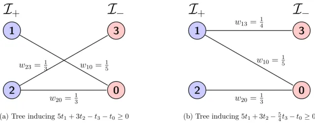
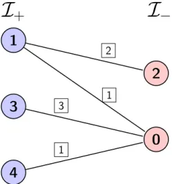
Example 2 Consider the set Q0 with disjuncts defined by the following inequalities 4t1 +3t2 −t3 −t0 ≥0
5t1 +t2 −2t3 −t0 ≥0 5t1 +2t2 −2t3 −t0 ≥0.
We have that I+ ={1,2} and I− ={3,0}. Further, edge weights can be computed to
be w13= 14,w10= 15, w23 = 13, w20 = 13.
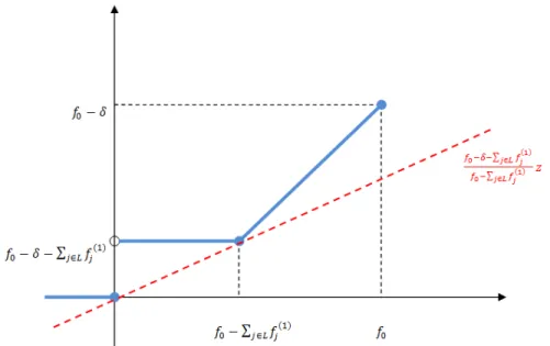
Two spanning trees of G are shown in Figure 2.1. The inequality induced by the
subtree of Figure 2.1(a) is5t1+ 3t2−t3−t0 ≥0. This inequality is the c-max cut and,
hence, is valid for cl conv(Q0). Furthermore, it can be verified to be facet-defining for
this set. The inequality induced by the subtree of Figure 2.1(b) is5t1+3t2−54t3−t0 ≥0,
which is not valid because it cuts off the feasible point (0,1,3,0)∈Q0
1 ⊆cl conv(Q0).
1
3
2
0
I
+
I
−
w10= 15 w23= 13 w20= 13(a) Tree inducing5t1+ 3t2−t3−t0≥0
1
3
2
0
I
+
I
−
w13= 14 w10= 15 w20= 13 (b) Tree inducing5t1+ 3t2−54t3−t0≥0Figure 2.1.: Spanning trees and induced inequalities for Example 2
Example 2 shows that not all spanning trees of G induce a valid inequality. The
reason is that the induced coefficients may violate an inequality corresponding to an edge that is not included in the spanning tree. We refer to a spanning tree that induces a valid inequality as afeasible spanning tree. We next show that any inequality
induced by a feasible spanning tree is facet-defining for cl conv(Q0).
Proposition 2.5.1 Inequality β|t≥0with β0 =−1is facet-defining for cl conv(Q0)
if and only if β is induced by a feasible spanning tree of G.
Proof Let β|t ≥ 0 with β
0 = −1 be a facet-defining inequality for cl conv(Q0).
of B2, it belongs to n = |V0| −1 hyperplanes of the form {β ∈ R|V0| : βj +wijβi =
0} whose coefficient vectors are linearly independent, in addition to β0 = −1. By
Proposition 2.4.2, the subgraph with respect to β forms a spanning tree of G.
For the converse, suppose β|t ≥0withβ0 =−1is induced by a feasible spanning
tree. The validity ofβ|t≥0follows directly from the definition of a feasible spanning
tree. By construction, see (2.17), coefficients β satisfy n equations of the form βj + wijβi = 0, one for each edge of the tree. Lemma 2 shows that thesencoefficient vectors
are independent. Therefore, β is an extreme point of B2. Hence, Theorem 2.3.1
implies that β|t≥0 is facet-defining for cl conv(Q0).
We next introduce the notion of label-connectivity. LetS be a spanning tree ofG
with edge setE ⊆ I+× I−. A functionL:E → L is called a label-function if
L({i, j})∈ l∈ L:fli >0,− flj fli =wij
for each {i, j} ∈ E. In words, L({i, j}) returns the index l of an inequality in the
description of Q0 with fli > 0 and the property that the ratio of the coefficient of tj over that of ti equals −wij. Because the ratio wij might be achieved in different
rows, several label-functions might be associated with a single spanning tree. For this reason, we define the set of all the label-functions of spanning tree S by L(S). We
writeS(E, L)to refer to a specific spanning tree with edge setE and label-functionL.
We say there is alabel-disconnection for labell inS(E, L)if the subgraph of S(E, L)
induced by the edges of label l is disconnected. It is easily seen that this definition is
equivalent to stating that there exists a path in S(E, L)where two edges with label l
are connected within the tree using a path whose edges do not have label l. Finally,
we say that a spanning tree S with edge set E is label-connected if there exists a
label-function L ∈ L(S) such that S(E, L) does not exhibit label-disconnection for
any l ∈ L. Otherwise it is label-disconnected.
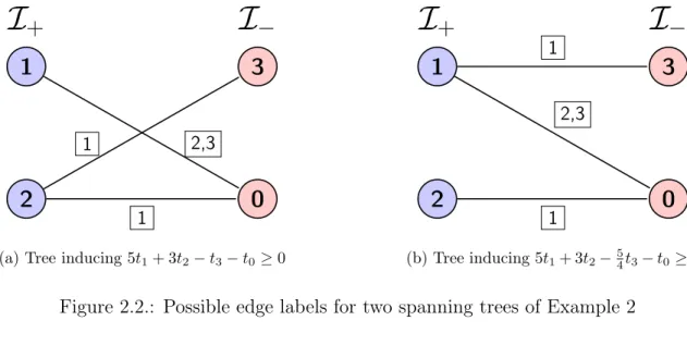
Example 2 (continued) In Figure 2.2, we add all possible valid edge labels to the edges of the spanning trees presented in Figure 2.1. In Figure 2.2(a), we observe that
1
3
2
0
I
+
I
−
2,3 1 1(a) Tree inducing5t1+ 3t2−t3−t0≥0
1
3
2
0
I
+
I
−
1 2,3 1 (b) Tree inducing5t1+ 3t2−54t3−t0≥0Figure 2.2.: Possible edge labels for two spanning trees of Example 2
there are two possible labels for edge {1,0}, each of which determines that w10 = 15.
We see that, independent of the choice of label for edge {1,0}, the spanning tree does not exhibit any label-disconnection. It is therefore label-connected. In Figure 2.2(b),
we observe that independent of the choice of label for edge {1,0}, the spanning tree
will exhibit a label-disconnection for label 1 along the path 3−1−0−2. We conclude
that this spanning tree is label-disconnected.
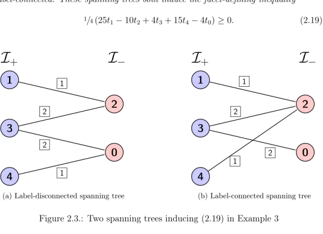
Label-connected spanning trees do not necessarily induce valid inequalities and not all feasible trees that induce a facet-defining inequality are label-connected. However, we show next via an example and later prove that, for facet-defining inequalities, there exists a feasible spanning tree that is label-connected.
Example 3 Consider the set Q0 with disjuncts defined by the following inequalities
25 4t1 − 5 2t2 + 5 16t3 + 15 4t4 −t0 ≥0 5t1 −52t2 +t3 +72t4 −t0 ≥0.
For this set, we have that I+ ={1,3,4}and I−={2,0}. We compute that w10 = 254 ,
w30 = 1, w40 = 154, w12 = 52, w32 = 52 and w42 = 23. Corresponding edge labels