The Rise and Fall of the Environmental Kuznets Curve

(1)

The Rise and Fall of the Environmental

Kuznets Curve

DAVID I. STERN

*

Rensselaer Polytechnic Institute, Troy, NY, USA

Available online

Summary. —This paper presents a critical history of the environmental Kuznets curve (EKC). The EKC proposes that indicators of environmental degradation first rise, and then fall with increasing income per capita. Recent evidence shows however, that developing countries are addressing environmental issues, sometimes adopting developed country standards with a short time lag and sometimes performing better than some wealthy countries, and that the EKC results have a very flimsy statistical foundation. A new generation of decomposition and efficient frontier models can help disentangle the true relations between development and the environment and may lead to the demise of the classic EKC.

Key words — environmental Kuznets curve, pollution, economic development, econometrics, review, global

1. INTRODUCTION

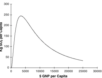
The environmental Kuznets curve (EKC) is a hypothesized relationship between various indicators of environmental degradation and income per capita. In the early stages of eco-nomic growth degradation and pollution increase, but beyond some level of income per capita, which will vary for diﬀerent indicators, the trend reverses, so that at high income levels economic growth leads to environmental improvement. This implies that the environ-mental impact indicator is an inverted U-shaped function of income per capita. Typically, the logarithm of the indicator is modeled as a quadratic function of the logarithm of income. An example of an estimated EKC is shown in Figure 1. The EKC is named for Kuznets (1955) who hypothesized that income inequality ﬁrst rises and then falls as economic development proceeds.

The EKC concept emerged in the early 1990s with Grossman and Krueger’s (1991) path-breaking study of the potential impacts of NAFTA and the concept’s popularization through the 1992 World Bank Development Report (IBRD, 1992). If the EKC hypothesis were true, then rather than being a threat to the environment, as claimed by the environmental

movement and associated scientists in the past (e.g., Meadows, Meadows, Randers, & Beh-rens, 1972), economic growth would be the means to eventual environmental improvement. This change in thinking was already underway in the emerging idea of sustainable economic development promulgated by the World Com-mission on Environment and Development (1987) inOur Common Future. The possibility of achieving sustainability without a signiﬁcant deviation from business as usual was an obvi-ously enticing prospect for many––letting

doi:10.1016/j.worlddev.2004.03.004

www.elsevier.com/locate/worlddev

*I thank Cutler Cleveland, Quentin Grafton and two anonymous referees, for comments on drafts of this manuscript. Participants at seminars at the University of Wollongong, Clark University, University of York, University of Cambridge, Rensselaer Polytechnic Insti-tute, and the Australian National University and at conferences organized by the Association of American Geographers in Los Angeles and the International Society for Ecological Economics in Sousse, Tunisia aided in developing my arguments. Additionally, I am grateful to my collaborators Mick Common, Roger Perman, and Kali Sanyal for their contributions dis-cussed in this paper. Final revision accepted: 23 March 2004.

(2)

humankind ‘‘have our cake and eat it’’ (Rees, 1990, p. 435).

The EKC is an essentially empirical phe-nomenon, but most of the EKC literature is econometrically weak. In particular, little or no attention has been paid to the statistical prop-erties of the data used––such as serial depen-dence or stochastic trends in time-series1––and little consideration has been paid to issues of model adequacy such as the possibility of omitted variables bias.2 Most studies assume that, if the regression coeﬃcients are nominally individually or jointly signiﬁcant and have the expected signs, then an EKC relation exists. However, one of the main purposes of doing econometrics is to test which apparent rela-tionships, or ‘‘stylized facts,’’ are valid and which are spurious correlations.

When we do take diagnostic statistics and specification tests into account and use appro-priate techniques, we find that the EKC does not exist (Perman & Stern, 2003). Instead, we get a more realistic view of the effect of eco-nomic growth and technological changes on environmental quality. It seems that emissions of most pollutants and flows of waste are monotonically rising with income, though the ‘‘income elasticity’’ is less than one and is not a simple function of income alone. Income-inde-pendent, time-related effects reduce environ-mental impacts in countries at all levels of income. The new (post-Brundtland) conven-tional wisdom that developing countries are ‘‘too poor to be green’’ (Martinez-Alier, 1995)

is, itself, lacking in wisdom. In rapidly growing middle-income countries, however the scale effect, which increases pollution and other degradation, overwhelms the time effect. In wealthy countries, growth is slower, and pol-lution reduction efforts can overcome the scale effect. This is the origin of the apparent EKC effect. The econometric results are supported by recent evidence that, in fact, pollution problems are being addressed and remedied in developing economies (e.g., Dasgupta, Laplante, Wang, & Wheeler, 2002).

This paper follows the development of the EKC concept in approximately chronological order. I do not attempt to review or cite all of the rapidly growing number of studies. The next two sections of the paper review in more detail the theory behind the EKC and the econometric methods used in EKC studies. The following sections review some EKC analyses and their critique. Sections 6 and 7 discuss the more important recent developments that have changed the picture that we have of the EKC. The final sections discuss alternative approa-ches––decomposition of emissions and efficient frontiers––and summarize the findings.

2. THEORETICAL BACKGROUND The EKC concept emerged in the early 1990s with Grossman and Krueger’s (1991) path-breaking study of the potential impacts of NAFTA and Shaﬁk and Bandyopadhyay’s

0 50 100 150 200 250 300 0 5000 10000 15000 20000 25000 30000 $ GNP per Capita Kg SO 2 per Capita

Figure 1.Environmental Kuznets curve for sulfur emissions. Source: Panayotou (1993) and Stern, Common, and Barbier (1996).

(3)

(1992) background study for the 1992 World Development Report. The EKC theme was popularized by the World Bank’s World Development Report 1992(IBRD, 1992), which argued that: ‘‘The view that greater economic activity inevitably hurts the environment is based on static assumptions about technology, tastes and environmental investments’’ (p. 38) and that ‘‘As incomes rise, the demand for improvements in environmental quality will increase, as will the resources available for investment’’ (p. 39). Others have expounded this position even more forcefully with Beck-erman (1992) claiming that ‘‘there is clear evi-dence that, although economic growth usually leads to environmental degradation in the early stages of the process, in the end the best––and probably the only––way to attain a decent environment in most countries is to become rich.’’ (p. 491). In his highly publicized and controversial book,The Skeptical Environmen-talist, Lomborg (2001) relies heavily on the 1992 World Development Report(Cole, 2003a) to argue the same point, while many environ-mental economists take the EKC as a stylized fact that needs to be explained by theory. All this is despite the fact that the EKC has never been shown to apply to all pollutants or envi-ronmental impacts and recent evidence,3 dis-cussed in this paper, challenges the notion of the EKC in general. The remainder of this section discusses the economic factors that drive changes in environmental impacts and may be responsible for rising or declining environmental degradation over the course of economic development.

If there were no change in the structure or technology of the economy, pure growth in the scale of the economy would result in growth in pollution and other environmental impacts. This is called the scale effect. The traditional view that economic development and environ-mental quality are conflicting goals reflects the scale effect alone. Proponents of the EKC hypothesis argue that

at higher levels of development, structural change to-wards information-intensive industries and services, coupled with increased environmental awareness, enforcement of environmental regulations, better technology and higher environmental expenditures, result in leveling oﬀ and gradual decline of environ-mental degradation (Panayotou, 1993, p. 1).

Thus there are both proximate causes of the EKC relationship––scale, changes in economic

structure or product mix, changes in techno-logy, and changes in input mix, as well as underlying causes such as environmental regu-lation, awareness, and education, which can only have an eﬀect via the proximate variables. Let us look in more detail at the proximate variables:

(a) Scale of production implies expanding production at given factor-input ratios, out-put mix, and state of technology. It is nor-mally assumed that a 1% increase in scale results in a 1% increase in emissions. This is because if there is no change in the in-put–output ratio or in technique there has to be a proportional increase in aggregate inputs. However, there could, in theory, be scale economies or diseconomies of pollu-tion (Andreoni & Levinson, 2001). Some pollution control techniques may not be practical at a small scale of production and vice versa or may operate more or less effectively at different levels of output. (b) Different industries have different pollu-tion intensities. Typically, over the course of economic development the output mix

changes. In the earlier phases of develop-ment there is a shift away from agriculture toward heavy industry which increases emissions, while in the later stages of devel-opment there is a shift from the more re-source intensive extractive and heavy industrial sectors toward services and light-er manufacturing, which supposedly have lower emissions per unit of output.4

(c) Changes ininput mixinvolve the substitu-tion of less environmentally damaging inputs for more damaging inputs and vice versa. Examples include: substituting natural gas for coal and substituting low sulfur coal in place of high sulfur coal. As scale, output mix, and technology are held constant, this is equivalent to moving along the isoquants of a neoclassical production function. (d) Improvements in thestate of technology

involve changes in both:

• Productivityin terms of using less,ceteris paribusof the polluting inputs per unit of output. A general increase in total factor productivity will result in lower emis-sions per unit of output even though this is not necessarily an intended conse-quence.

• Emissions speciﬁc changes in process re-sult in lower emissions per unit of input. These innovations are speciﬁcally in-tended to reduce emissions.5

(4)

This framework applies most directly to emissions of pollutants. For concentrations of pollutants, decentralization of economic activity with development is also important (Sternet al., 1996). Deforestation is also a ﬂow of envi-ronmental degradation. Improved technology would imply more replanting, selective cutting, wood recovery etc. that reduces deforestation per unit wood produced. Stock pollutants or impacts need a diﬀerent, dynamic framework.

Though any actual change in the level of pollution must be a result of change in one of the proximate variables, those variables may be driven by changes in underlying variables that also vary over the course of economic devel-opment. A number of papers have developed theoretical models of how preferences and technology might interact to result in different time paths of environmental quality. The vari-ous studies make different simplifying assump-tions about the economy. Most of these studies can generate an inverted U-shape curve of pollution intensity but there is no inevitability about this. The result depends on the assump-tions made and the values of particular parameters. Lopez (1994) and Selden and Song (1995) assume infinitely lived agents, exogenous technological change and that pollution is generated by production and not by consump-tion. John and Pecchenino (1994), John, Pec-chenino, Schimmelpfennig, and Schreft (1995), and McConnell (1997) develop models based on overlapping generations where pollution is generated by consumption rather than by pro-duction activities. In addition, Stokey (1998) allows endogenous technical change and Lieb (2001) generalizes Stokey’s (1998) model, arguing that satiation in consumption is needed to generate the EKC. Finally, Ansuategi and Perrings (2000) incorporate transboundary externalities. Magnani (2001) discusses how individual preferences are converted into public policy. Andreoni and Levinson (2001) argue that none of these special assumptions is needed and economies of scale in abatement are sufficient to generate the EKC. Most studies model the emission of pollutants. Lopez (1994) and Bulte and van Soest (2001), among others, develop models for the depletion of natural resources such as forests or agricultural land fertility. It seems easy to develop models that generate EKCs under appropriate assumptions. None of these theoretical models has been tested empirically. Furthermore, if, in fact, the EKC for emissions is monotonic, as more recent evidence suggests, the ability of a model

to produce an inverted U-shaped curve is not a particularly desirable property.

3. ECONOMETRIC FRAMEWORK The earliest EKCs were simple quadratic functions of the levels of income. But, eco-nomic activity inevitably implies the use of resources and, by the laws of thermodynamics, use of resources inevitably implies the produc-tion of waste. Regressions that allow levels of indicators to become zero or negative are inappropriate except in the case of deforesta-tion where aﬀorestadeforesta-tion can occur. A logarith-mic dependent variable will impose this restriction. Some studies, including the original Grossman and Krueger (1991) paper, used a cubic EKC in levels and found an N-shape EKC. This might just be a polynomial approximation to a logarithmic curve. The standard EKC regression model is, therefore: lnðE=PÞit¼aiþctþb1lnðGDP=PÞit

þb2ðlnðGDP=PÞÞ 2

itþeit; ð1Þ

where E is emissions, P is population, and ln indicates natural logarithms. The first two terms on the RHS are intercept parameters which vary across countries or regions i and yearst. The assumption is that, though the level of emissions per capita may differ over coun-tries at any particular income level, the income elasticity is the same in all countries at a given income level. The time specific intercepts account for time-varying omitted variables and stochastic shocks that are common to all countries. The ‘‘turning point’’ income, where emissions or concentrations are at a maximum, is given by:

s¼expðb₁=ð2b₂ÞÞ: ð2Þ

Usually the model is estimated with panel data. Most studies attempt to estimate both the fixed and random-effects models. The fixed-effects model treats the ai andct as regression

parameters. The random-eﬀects model treats the ai and ct as components of the random

disturbance. If the eﬀects ai and ct and the

explanatory variables are correlated, then the random-effects model cannot be estimated consistently (Hsiao, 1986). Only the fixed-effects model can be estimated consistently. A Hausman (1978) test can be used to test for inconsistency in the random-effects estimate by comparing the fixed-effects and random-effects

(5)

slope parameters. A significant difference indi-cates that the random-effects model is estimated inconsistently, due to correlation between the explanatory variables and the error compo-nents. Assuming that there are no other statis-tical problems, the fixed-effects model can be estimated consistently, but the estimated parameters are conditional on the country and time effects in the selected sample of data (Hsiao, 1986). Therefore, they cannot be used to extrapolate to other samples of data. This means that an EKC estimated with fixed-effects using only developed country data might say little about the future behavior of developing countries. Many studies compute the Hausman statistic and, finding that the random-effects model cannot be consistently estimated, esti-mate the fixed-effects model. But few have pondered the deeper implications of the failure of this orthogonality test.

GDP may be an integrated variable. If the EKC regressions do not cointegrate, then the estimates will be spurious. Until recently, very few studies have reported any diagnostic sta-tistics for integration of the variables or coin-tegration of the regressions. Therefore, it is unclear what we can infer from the majority of EKC studies. Testing for integration and coin-tegration in panel data is a rapidly developing field. Perman and Stern (2003) employ some of these tests and find that sulfur emissions and GDP per capita may be integrated variables. The unit root hypothesis could be rejected for sulfur (but not GDP) using the Im, Pesaran, and Shin (2003) (IPS) test when the alternative was trend stationarity. But alternative hypotheses and tests result in acceptance of the unit root hypothesis. Heil and Selden (1999) find the same result for carbon dioxide emissions and GDP using the IPS test. But they prefer results that allow for a structural break 1974, in which allows them to strongly reject the unit root hypothesis for both GDP and carbon. Coondoo and Dinda (2002) yield similar results to Per-man and Stern (2003) for carbon dioxide emis-sions. de Bruyn (2000) and Day and Grafton (2003) carry out time-series unit root tests for the Netherlands, the United Kingdom, the United States, West Germany, and Canada for a variety of pollutants with very similar results.

4. RESULTS OF EKC STUDIES Many basic EKC models relating environ-mental impacts to income without additional

explanatory variables have been estimated. But the key features differentiating the models for different pollutants, data etc. can be displayed by reviewing a few of the early studies and examining a single impact in more detail. I review the contributions of Grossman and Krueger (1991), Shafik (1994), and Selden and Song (1994) and then look in more detail at studies for sulfur pollution and emissions. Finally, I briefly discuss studies that estimate an EKC for energy use.

Many EKC studies have also been published that include additional explanatory additional explanatory variables, intended to model underlying or proximate factors, such as ‘‘political freedom’’ (e.g., Torras & Boyce, 1998) or output structure (e.g., Panayotou, 1997), or trade (e.g., Suri & Chapman, 1998). Stern (1998) reviews several of these. In general, the included variables turn out to be significant at traditional significance levels. Testing different variables individually is however subject to the problem of potential omitted variables bias. Further, these studies do not report cointegra-tion or other statistics that might tell us if omitted variables bias is likely to be a problem or not. Therefore, it is not clear what we can infer from this body of work. Given these problems, I do not review these studies sys-tematically here.

To some (e.g., Lopez, 1994) the early EKC studies indicated that local pollutants were more likely to display an inverted U-shape relation with income, while global impacts such as carbon dioxide did not. This picture ﬁts environmental economics theory––local impacts are internalized within a single economy or region and are likely to give rise to environ-mental policies to correct the externalities on pollutees before such policies are applied to globally externalized problems. But as we will see, the picture is not quite so clear cut even in the early studies. Furthermore, the more recent evidence on sulfur and carbon dioxide emis-sions shows there may be no strong distinction between the eﬀect of income per capita on local and global pollutants. Stern et al. (1996) determined that higher turning points were found for regressions that used purchasing power parity (PPP) adjusted income compared to those that used market exchange rates and for studies using emissions of pollutants rela-tive to studies using ambient concentrations in urban areas. In the initial stages of economic development urban and industrial development tends to become more concentrated in a smaller

(6)

number of cities which also have rising central population densities. Many developing coun-tries have a ‘‘primate city’’ that dominates a country’s urban hierarchy and contains much of its modern industry––Bangkok is one of the best such examples. In the later stages of eco-nomic development, urban and industrial development tends to decentralize. Moreover, the high population densities of less-developed cities are gradually reduced by suburbaniza-tion. So, it is possible for peak ambient pollu-tion concentrapollu-tions to fall as income rises even if total national emissions are rising.

The ﬁrst empirical EKC study was the NBER working paper by Grossman and Krue-ger (1991) 6that estimated EKCs for SO2, dark

matter (ﬁne smoke), and suspended particles (SPM) using the GEMS dataset as part of a study of the potential environmental impacts of NAFTA. The GEMS dataset is a panel of ambient measurements from a number of locations in cities around the world. Each regression involved a cubic function in levels (not logarithms) of PPP per capita GDP and various site-related variables, a time trend, and a trade intensity variable. The turning points for SO2 and dark matter were at around

$4,000–5,000 while the concentration of sus-pended particles appeared to decline even at low income levels. At income levels over $10,000–15,000, Grossman and Krueger’s esti-mates show increasing levels of all three pollu-tants.

The results of Shafik and Bandyopadhyay’s (1992)7 _{study were used in the 1992} _World Development Report (IBRD, 1992) and were, therefore, particularly influential. They esti-mated EKCs for 10 different indicators using three different functional forms: linear, quadratic and, in the most general case, a log-arithmic cubic polynomial in PPP GDP per capita as well as a time-trend and site-related variables. In each case, the dependent variable was untransformed. They found that lack of clean water and lack of urban sanitation decline uniformly with increasing income, and over time. Both measures of deforestation were found to be insignificantly related to the income terms. River quality tended to worsen with increasing income. The two air pollutants, however, conform to the EKC hypothesis. The turning points for both pollutants were at income levels of between $3,000 and $4,000. Finally, both municipal waste and carbon emissions per capita increased unambiguously with rising income.

Selden and Song (1994) estimated EKCs for four emissions series: SO2, NOx, SPM, and CO

using longitudinal data primarily from devel-oped countries. The estimated turning points were all very high compared to the two earlier studies. For the fixed-effects version of their model they were (converted to US$1,990 using the US GDP implicit price deflator): SO2,

$10,391; NOx, $13,383; SPM, $12,275; and CO,

$7,114. This study showed that the turning point for emissions was likely to be higher than that for ambient concentrations.

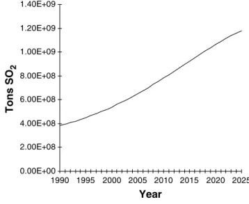
Table 1 summarizes several studies of sulfur emissions and concentrations, listed in order of estimated income turning point. Panayotou (1993) used cross-sectional data, nominal GDP, and the assumption that the emission factor for each fuel is the same in all countries––this study has the lowest estimated turning point of all. With the exception of the Kaufmann et al. (1998) estimate, all turning point estimates using concentration data are less than $6,000. Kaufmannet al. (1998) used an unusual speci-ﬁcation that includes GDP per area and GDP per area squared variables.

Among the emissions based estimates, both Selden and Song (1994) and Coleet al. (1997) used databases dominated by, or consisting solely of, emissions from OECD countries. Their estimated turning points are $10,391 and $8,232 respectively. List and Gallet (1999) used data for the 50 US states from 1929–94. Their estimated turning point is the second highest in the table. Income per capita in their sample ranges from $1,162 to $22,462 in 1987 US dollars. This is a greater range of income levels than is found in the OECD-based panels for recent decades. This suggests that including more low-income data points in the sample might yield a higher turning point. Stern and Common (2001) estimated the turning point at over $100,000. They used an emissions data-base produced for the US Department of Energy by ASL (Lefohn, Husar, & Husar, 1999) that covers a greater range of income levels and includes more data points than any of the other sulfur EKC studies.

We see that the recent studies that used more representative samples ﬁnd that there is a monotonic relation between sulfur emissions and income just as there is between carbon dioxide and income. Interestingly, Dijkgraaf and Vollebergh (1998) estimate a carbon EKC for a panel data set of OECD countries ﬁnd-ing an inverted U-shape EKC in the sample as a whole (as well as many signs of poor

(7)

Table 1. Sulfur EKC studies

Authors Turning point 1990 USD

Emissions or concentrations

PPP Additional variables

Data source for sulfur

Time period Countries/cities

Panayotou (1993) $3,137 Emissions No – Own estimates 1987–88 55 developed and developing

countries Shaﬁk (1994) $4,379 Concentrations Yes Time trend,

loca-tional dummies

GEMS 1972–88 47 cities in 31 countries Torras and Boyce

(1998)

$4,641 Concentrations Yes Income inequal-ity, literacy, political and civil

rights, urbaniza-tion, locational

dummies

GEMS 1977–91 Unknown num-ber of cities in 42 countries Grossman and Krueger (1991) $4,772–5,965 Concentrations No Locational dummies, popu-lation density, trend GEMS 1977, ‘82, ‘88 Up to 52 cities in up to 32 coun-tries

Panayotou (1997) $5,965 Concentrations No Population density, policy

variables

GEMS 1982–84 Cities in 30 loped and deve-loping countries Cole, Rayner, and

Bates (1997)

$8,232 Emissions Yes Country dummy, technology level

OECD 1970–92 11 OECD countries Selden and Song

(1994)

$10,391–10,620 Emissions Yes Population density WRI––primarily OECD source 1979–87 22 OECD and 8 developing countries Kaufmann, Davidsdottir, Garnham, and Pauly (1998)

$14,730 Concentrations Yes GDP/Area, steel exports/GDP

UN 1974–89 13 developed and 10 developing

countries

List and Gallet (1999)

$22,675 Emissions N/A – US EPA 1929–94 US States

Stern and Common (2001)

$101,166 Emissions Yes Time and coun-try eﬀects

ASL 1960–90 73 developed and developing coun-tries THE ENVIRON MENTAL KUZNET S CURVE 1425

(8)

econometric behavior). The turning point is at only 54% of maximal GDP in the sample. A study by Schmalensee, Stoker, and Judson (1998) also finds a within sample turning point for carbon. In this case, a 10-piece spline was fitted to the data such that the coefficient esti-mates for high-income countries are allowed to vary from those for low-income countries. All these studies suggest that the differences in turning points that have been found for differ-ent pollutants may be due, at least partly, to the different samples used. I will discuss the econometric reasons for this sample-dependent behavior below.

In an attempt to capture all environmental impacts of whatever type, a number of researchers (e.g., Suri & Chapman, 1998; Cole

et al., 1997) have estimated EKCs for a proxy total environmental impact indicator––total energy use. In each case, they found that energy use per capita increases monotonically with income per capita. This result does not preclude the possibility that energy intensity––energy used per dollar of GDP produced––declines with rising income or even follows an inverted U-shaped path (e.g., Galli, 1998).

The only robust conclusions from the EKC literature appear to be that concentrations of pollutants may decline from middle income levels, while emissions tend to be monotonic in income. As we will see below, emissions may decline simultaneously over time in countries at widely varying levels of development. Given the poor statistical properties of most EKC mod-els, it is hard to come to any conclusions about the roles of other additional variables such as trade. Too few quality studies have been done of other indicators apart from air pollution to come to any ﬁrm conclusions about those impacts either.

5. THEORETICAL CRITIQUE OF THE EKC

A number of critical surveys of the EKC literature have been published (e.g., Ansuategi, Barbier, & Perrings, 1998; Arrow et al., 1995; Copeland & Taylor (2004); Dasgupta et al., 2002; Ekins, 1997; Pearson, 1994; Stern, 1998; Stern et al., 1996). This section discusses the criticisms raised against the EKC in the earlier surveys on theoretical (rather than methodo-logical) grounds. The more recent surveys raise similar points but have more evidence to mar-shal.

The key criticism of Arrowet al. (1995) and others was that the EKC model, as presented in the 1992 World Development Report and else-where, assumes that there is no feedback from environmental damage to economic production as income is assumed to be an exogenous var-iable. The assumption is that environmental damage does not reduce economic activity suﬃciently to stop the growth process and that any irreversibility is not so severe that it reduces the level of income in the future. In other words, there is an assumption that the economy is sustainable. But, if higher levels of economic activity are not sustainable, attempting to grow fast in the early stages of development when environmental degradation is rising may prove counterproductive.8

It is clear that emissions of many pollutants per unit of output have declined over time in developed countries with increasingly stringent environmental regulations and technical inno-vations. But the mix of residuals has shifted from sulfur and nitrogen oxides to carbon dioxide and solid waste so that aggregate waste is still high and per capita waste may not have declined.9 Economic activity is inevitably environmentally disruptive in some way. Sat-isfying the material needs of people requires the use and disturbance of energy ﬂows and mate-rials stocks. Therefore, an eﬀort to reduce some environmental impacts may just aggravate other problems.10

Both Arrow et al. (1995) and Stern et al. (1996) argued that, if there was an EKC type relationship, it might be partly or largely a result of the effects of trade on the distribution of polluting industries. The Hecksher-Ohlin trade theory suggests that, under free trade, developing countries would specialize in the production of goods that are intensive in the factors that they are endowed with in relative abundance: labor and natural resources. The developed countries would specialize in human capital and manufactured capital intensive activities. Part of the reduction in environ-mental degradation levels in the developed countries and increases in environmental deg-radation in middle income countries may reflect this specialization (Hettige, Lucas, & Wheeler, 1992; Lucas, Wheeler, & Hettige, 1992; Suri & Chapman, 1998). Environmental regulation in developed countries might further encourage polluting activities to gravitate toward the developing countries (Lucaset al., 1992). These effects would exaggerate any apparent decline in pollution intensity with rising income along

(9)

the EKC. In our finite world the poor countries of today would be unable to find further countries from which to import resource-intensive products as they, themselves, become wealthy. When the poorer countries apply similar levels of environmental regulation they would face the more difficult task of abating these activities rather than outsourcing them to other countries (Arrowet al., 1995; Sternet al., 1996). Copeland and Taylor (2004) conclude that, in contrast to earlier work (e.g., Jaffe, Peterson, Portney, & Stavins, 1995), recent research shows that increased regulation does tend to result in more decisions to locate in less regulated locations. On the other hand, there is no clear evidence that trade liberalization results in a shift in polluting activities to less-regulated countries.

Furthermore, Antweiler, Copeland, and Taylor (2001) and Cole and Elliott (2003) argue that the capital-intensive activities that are concentrated in the developed countries are more polluting and hence developed countries have a natural comparative advantage in pol-luting goods in the absence of regulatory dif-ferences. There are no clear answers on the impact of trade on pollution from the empirical EKC literature.

Stern et al. (1996) argued that early EKC studies showed that a number of indicators: SO2emissions, NOx, and deforestation, peak at

income levels around the current world mean per capita income. A cursory glance at the

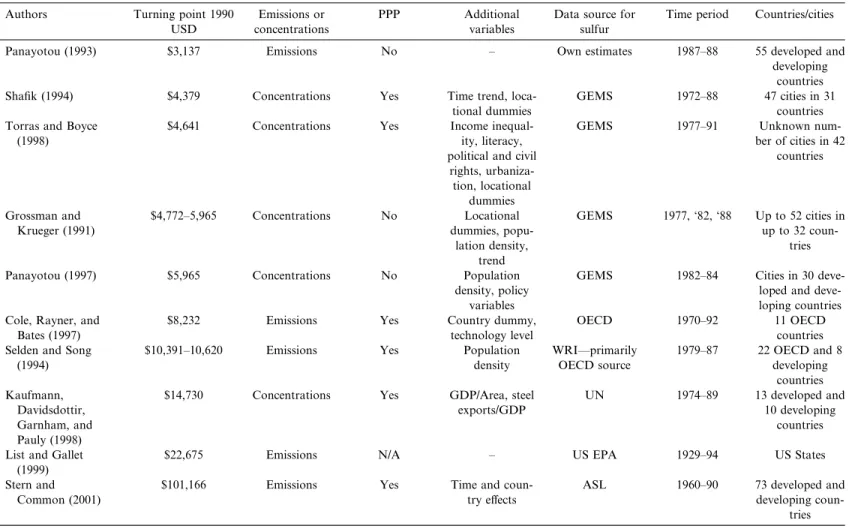
available econometric estimates might have lead one to believe that, given likely future levels of mean income per capita, environmen-tal degradation should decline from the present onward. This interpretation is evident in the 1992World Development Report(IBRD, 1992). Income is not however, normally distributed but very skewed, with much larger numbers of people below mean income per capita than above it. Therefore, it is median rather than mean income that is the relevant variable. Sel-den and Song (1994) and Stern et al. (1996) performed simulations that, assuming that the EKC relationship is valid, showed that global environmental degradation was set to rise for a long time to come. Figure 2 presents projected sulfur emissions using the EKC in Figure 1 and UN and World Bank forecasts of economic and population growth. Despite this and despite recent estimates that indicate higher or nonex-istent turning points, the impression produced by the early studies in the policy, academic, and business communities seems slow to fade (e.g., Lomborg, 2001).

6. RECENT DEVELOPMENTS Signiﬁcant developments, since my last gen-eral survey of the EKC in 1998, fall into three classes: (a) Empirical case study evidence on environmental performance and policy in developing countries that is discussed in this

0.00E+00 2.00E+08 4.00E+08 6.00E+08 8.00E+08 1.00E+09 1.20E+09 1.40E+09 1990 1995 2000 2005 2010 2015 2020 2025 Year Tons SO 2

Figure 2.Projected sulfur emissions. Source: Stern et al. (1996).

(10)

section; (b) improved econometric testing and estimates discussed in the following section; and (c) a new wave in the investigation of environment-development relations using de-composition analysis and eﬃcient frontier methods, discussed in Section 8.

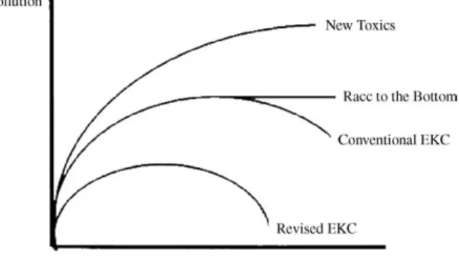
Dasguptaet al. (2002) wrote a critical review of the EKC literature and other evidence on the relation between environmental quality and economic development in the Journal of Eco-nomic Perspectives. Figure 3 illustrates four alternative viewpoints discussed in the article regarding the nature of the emissions and income relation. The conventional EKC needs no further discussion. Two viewpoints argue that the EKC is monotonic. The ‘‘new toxics’’ scenario claims that while some traditional pollutants might have an inverted U-shape curve, the new pollutants that are replacing them do not. These include carcinogenic chemicals, carbon dioxide, etc. As the older pollutants are cleaned up, new ones emerge, so that overall environmental impact is not reduced. The ‘‘race to the bottom’’ scenario posits that emissions were reduced in developed countries by outsourcing dirty production to developing countries. These countries will ﬁnd it harder to reduce emissions. But the pressure of globalization may also preclude further tightening of environmental regulation in developed countries and may even result in its loosening in the name of competitiveness.

The revised EKC scenario does not reject the inverted U-shape curve but suggests that it is shifting downward and to the left over time due to technological change. But this argument is already present in the1992 World Development Report (IBRD, 1992). Dasgupta et al. also

review the theoretical literature and some of the econometric speciﬁcation issues. But their main contribution is presenting evidence that envi-ronmental improvements are possible in devel-oping countries and that peak levels of environmental degradation will be lower than in countries that developed earlier.

According to Dasguptaet al. (2002), regula-tion of polluregula-tion and enforcement increase with income but the greatest increases happen from low to middle income levels and increased regulation is expected to have diminishing returns. There is also informal or decentralized regulation in developing countries––Coasian bargaining. Further, liberalization of develop-ing economies over the last two decades has encouraged more eﬃcient use of inputs and less subsidization of environmentally damaging activities––globalization is in fact good for the environment. The evidence seems to contradict the ‘‘race to the bottom’’ scenario. Multi-national companies respond to investor and consumer pressure in their home countries and raise standards in the countries in which they invest. Further, better methods of regulating pollution such as market instruments are hav-ing an impact even in develophav-ing countries. Better information on pollution is available, encouraging government to regulate and empowering local communities. Those that argue that there is no regulatory capacity in developing countries seem to be wrong.

Much of the Dasguptaet al. evidence is from China. Other researchers of environmental and economic developments in China come to similar conclusions. Gallagher (2003) ﬁnds that China is adopting European Union standards for pollution emissions from cars with an

Figure 3.Environmental Kuznets curve: alternative views. Source: Dasgupta et al. (2002) and Perman and Stern (2003).

(11)

approximately 8–10-year lag. Clearly, China’s income per capita is far more than 10 years behind that of Western Europe. Streets et al. (2001), Zhang (2000), Jiang and McKibbin (2002), and Wang and Wheeler (2003) all report on substantial reductions of pollution intensi-ties and levels in recent years.

7. ECONOMETRIC CRITIQUE OF THE EKC

Econometric criticisms of the EKC fall into four main categories: heteroskedasticity, simul-taneity, omitted variables bias, and cointegra-tion issues.

Stern et al. (1996) raised the issue of heter-oskedasticity that may be important in the context of regressions of grouped data (see Maddala, 1977). Schmalensee et al. (1998) found that regression residuals from OLS were heteroskedastic with smaller residuals associ-ated with countries with higher total GDP and population as predicted by Sternet al. (1996). Stern (2002) estimated a decomposition model using feasible GLS. Adjusting for hetero-skedasticity in the estimation significantly improved the goodness of fit of globally aggregated fitted emissions to actual emissions. Coleet al. (1997) and Holtz-Eakin and Sel-den (1995) used Hausman tests for regressor exogeneity to directly address the simultaneity issue. They found no evidence of simultaneity. In any case, simultaneity bias is less serious in models involving integrated variables than in

the traditional stationary econometric model (Perman & Stern, 2003). Coondoo and Dinda (2002) test for Granger Causality between CO2

emissions and income in various individual countries and regions. As the data are differ-enced to ensure stationarity, this test can only address short-run effects. The overall pattern that emerges is that causality runs from income to emissions or there is no significant relation-ship in developing countries, while in developed countries causality runs from emissions to income. This suggests that simultaneity is not important.

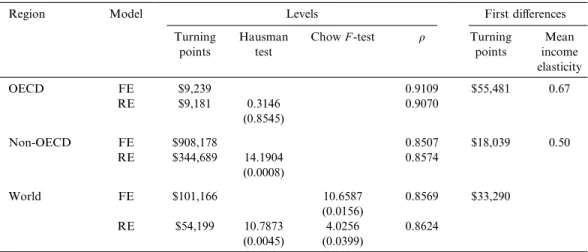
Stern and Common (2001) use three lines of evidence to suggest that the EKC is an inade-quate model and that estimates of the EKC in levels can suffer from significant omitted vari-ables bias: (a) Differences between the para-meters of the random-effects and fixed-effects models, tested using the Hausman test; (b) differences between the estimated coefficients in different subsamples, and (c) tests for serial correlation. Table 2 presents the key results from an EKC model estimated with data from 74 countries (in the World sample) over 1960– 90. For the non-OECD and World samples, the Hausman test shows a significant difference in the parameter estimates for the random-effects and fixed-effects model. This indicates that the regressors––the level and square of the loga-rithm of income per capita––are correlated with the country effects and time effects. As these effects model the mean effects of omitted vari-ables that vary across countries or across time, this indicates that the regressors are likely

Table 2. Stern and Common (2001) key results

Region Model Levels First diﬀerences

Turning points

Hausman test

ChowF-test q Turning points Mean income elasticity OECD FE $9,239 0.9109 $55,481 0.67 RE $9,181 0.3146 (0.8545) 0.9070 Non-OECD FE $908,178 0.8507 $18,039 0.50 RE $344,689 14.1904 (0.0008) 0.8574 World FE $101,166 10.6587 (0.0156) 0.8569 $33,290 RE $54,199 10.7873 (0.0045) 4.0256 (0.0399) 0.8624

All turning points in real 1990 purchasing power parity US dollars.

(12)

correlated with omitted variables and the regression coefficients are biased.11The OECD results pass this Hausman test but this result turned out to be very sensitive to the exact sample of countries included in the subsample. As expected, given the Hausman test results, the parameter estimates are dependent on the sample used, with the non-OECD estimates showing a turning point at extremely high-income levels and the OECD estimates a within sample turning point (Table 2). As mentioned above, these results exactly parallel those for developed and developing country samples of carbon emissions. The Chow F-test tests whether the two subsamples can be pooled, and therefore that there is a common regression parameter vector, a hypothesis that is rejected. The parameter q is the first order autore-gressive coefficient of the regression residuals. This level of serial correlation indicates mis-specification either in terms of omitted vari-ables or missing dynamics.

Harbaughet al. (2002) carry out a sensitivity analysis of the original Grossman and Krueger (1995) results. They use an updated and larger version of the ambient pollution data set and test a number of alternative specifications. Using the new extended dataset with Grossman and Krueger’s original cubic specification results in the coefficients changing sign and peak and trough levels altering wildly. Altering the specification in various ways––adding explanatory variables, using time dummies instead of a time trend, using logs, removing outliers, and averaging the observations across monitors in each country––changes the shape of the curve. The final experiment they carry out is to include only countries with GDP per capita above $8,000. In contrast to Stern and Common (2001), this results in a monotonic curve. The authors comment:

This may seem counterintuitive. SO2concentrations in Canada and the United States have declined over time at ever decreasing rates. . .the regressions. . .include. . . a linear time trend. . .after detrending the data with the time function, pollution appears to increase as a function of GDP (p. 548).

There are several differences between the Harbaughet al. (2002) model and the Stern and Common (2001) model that may explain the different results obtained for high income countries. Harbaugh et al. (2002) use concen-trations data, a linear time trend and a dynamic specification, while Stern and Common (2001)

use emissions data, individual time dummies, and a static specification. Stern and Common’s (2001) first differences results (Table 2) are very similar to the Harbaugh et al.’s (2002) results, which suggests that the dynamic specification could be important.

Millimet, List, and Stengos (2003) use a dif-ferent strategy to test the robustness of the parametric EKC––comparing it to semi-para-metric curves estimated using the same dataset for US states used by List and Gallet (1999). But they claim that parametric models are too pessimistic––finding high turning points––while their alternative semi-parametric models result in U-shaped curves with lower turning points. In addition, they reject the parametric specifi-cation in favor of the semi-parametric. But neither parametric nor semi-parametric curves seem to fit the observed data very well in the figures presented in the paper. Furthermore, results for individual states are varied, with the nitrogen dioxide curves mostly rising through-out the income range and many of the sulfur dioxide curves falling––the reverse of the national panel data results. These results could, therefore, be further evidence of the fragility of the EKC rather than evidence for a low turning point semi-parametric specification.

In contrast to Harbaughet al. (2002), Cole (2003b) claims that the EKC model is fairly robust. But his basic levels sulfur emissions EKC has a significant Hausman statistic for a test of whether the random and fixed-effects parameters differ. Adding trade variables to the model results in an insignificant Hausman sta-tistic and a somewhat higher turning point. Using logarithms increases this turning point further (Stern, 2004). The sulfur series cannot be tested for unit roots, but other series in the dataset he uses do show unit root behavior and results using first differences indicate a higher turning point than the levels results. I conclude that the model with trade variables performs better but the basic EKC is misspecified and appropriate econometric techniques appear to raise the turning point.

Perman and Stern (2003) test Stern and Common’s (2001) data and models for unit roots and cointegration respectively. Panel unit root tests indicate that all three series––log sulfur emissions per capita, log GDP capita, and its square––have stochastic trends. Results for cointegration are less clear cut. Around half the individual country EKC regressions coin-tegrate, but many of these have parameters with ‘‘incorrect signs.’’ Some panel

(13)

cointegra-tion tests indicate cointegracointegra-tion in all countries and some accept the noncointegration hypoth-esis. But even when cointegration is found, the form of the EKC relationship varies radically across countries with many countries having U-shaped EKCs. A common cointegrating vector for all countries is strongly rejected. Koop and Tole (1999) similarly found that random and fixed-effects specifications of a deforestation EKC were strongly rejected in favor of a random coefficients model with widely varying coefficients and insignificant mean coefficients.

In the presence of possible noncointegration, we can estimate a model in first differences. The estimated turning points indicate a largely monotonic EKC relationship and are more similar across subsamples, though the para-meters are still significantly different (Table 2). The estimated income elasticity is less than one––there are factors that change with income which offset the scale effect, but they are insufficiently powerful to overcome fully the scale effect.

Figure 4 presents the time effects from the first difference estimates. The OECD saw declining emissions holding income constant over the entire period, though the introduction of the LRTAP agreement in the mid-1980s in Europe resulted in a larger decline. Developing

countries saw rising emissions in the 1960s and declining emissions since 1973,ceteris paribus. Similarly, Lindmark (2002) uses the Kalman ﬁlter to extract a technological change trend for carbon dioxide emissions in Sweden from 1870–1997. This trend had a positive growth rate until about 1970 and a negative growth rate since.12

Day and Grafton (2003) test for cointegra-tion of the EKC relacointegra-tion using Canadian time-series data on a number of pollutants using the Engle-Granger and Johansen methods. They fail to reject the noncointegration hypothesis in almost every case. de Bruyn’s (2000) time-series Engle-Granger tests for the Netherlands, the United Kingdom, the United States, and West Germany for SOx, NOx and CO2 ﬁnds

cointe-gration for the CO2 EKC in the Netherlands

and West Germany, but not in any other case. Using various lines of evidence, the majority of studies have found the EKC to be a fragile model suﬀering from severe econometric mis-speciﬁcation. Use of more appropriate methods tends to indicate higher turning points and possibly a monotonic curve for emissions of major pollutants. A better model may result from including additional variables to represent either proximate or underlying causes of change in emissions. I next turn to a consideration of

-0.3 -0.2 -0.1 0 0.1 0.2 0.3 1960 1965 1970 1975 1980 1985 1990 World OECD Non-OECD

Figure 4.Time effects: first differences sulfur EKC. Source: Stern and Common (2001).

(14)

a new literature that goes beyond the EKC in this way.

8. DECOMPOSING EMISSIONS AND MEASURING ENVIRONMENTAL

EFFICIENCY

Two alternative approaches are emerging that go beyond the EKC by analyzing the proximate factors driving changes in pollution emissions described in Section 2: index number decompositions of emissions and production frontiers estimated using linear programming or econometrics. The index numbers decom-position approach requires detailed sectoral information on fuel use, production, emissions etc. The average eﬀects of the diﬀerent factors can be derived from the results for the indi-vidual countries. No stochasticity is allowed for. By contrast, the frontier models do not usually require data on fuel use by sector; they can estimate factors common to all countries as well as idiosyncratic components for each country, and the econometric versions allow for random error. On the other hand, the frontier models usually make stronger assumptions about production relations. There are also studies that are hybrids of the two approaches (e.g., Hettige, Mani, & Wheeler, 2000; Hilton & Levinson, 1998; Judsonet al., 1999).13 Gross-man (1995) and de Bruyn (1997) proposed the following decomposition:

Eit

Xn j¼1

YitIijtSijt; ð3Þ

whereEitis emissions in countryiin yeart,Y is

GDP, Ij is the emissions intensity of sector j,

andSjis the share of that sector in GDP. This

decomposition, therefore, attributes emissions to what Grossman calls the scale, composition (output mix), and technique effects. The latter includes the effects of both fuel mix and ‘‘technological change’’ and the latter can be further broken down into general productivity improvements, where more output is derived from a unit of input, and emissions reducing technological change, where less emissions are produced per unit of input. A problem for the index number studies is that, usually, fuel use data are collected on a different sectoral basis than output. This makes the standard type of index number study impossible to implement in most countries. Hamilton and Turton’s (2002) and Zhang’s (2000) index number

decomposi-tions of CO2emissions do not however

explic-itly include fuel mix or output structure and so do not require industry level data. This decomposition is given by:

Et Et FECt FECt TECt TECt GDPt GDPt Pt Pt; ð4Þ

whereEis emissions, FEC and TEC are fossil fuel and total energy consumption respectively, and P is population. As carbon abatement technologies do not yet exist, the first term on the RHS reflects the impact of shifts in the mix of fossil fuel types. The second term reflects shifts between fossil and nonfossil fuels, while the remaining terms are energy intensity and two components of the scale effect.

De Bruyn (1997), Viguier (1999), Selden, Forrest, and Lockhart (1999), and Bruvoll and Medin (2003) all calculate versions of (3) for a variety of European countries and the United States. A progressively larger number of pol-lutants have been investigated. de Bruyn (1997) only analyzes sulfur, while Bruvoll and Medin (2003) cover 10 pollutants. Output structure eﬀects are mostly small except for some of the additional pollutants investigated by Bruvoll and Medin (2003) (CH4, N2O, and NH3). Fuel

mix eﬀects are varied depending on the pollu-tants and countries investigated––in some cases they act to increase emissions (for SOx, NOx,

and CO2 in the US) and in others to reduce

emissions (SOx and CO2 in Norway). In all

cases, technique effects were dominant in off-setting the increase in scale. Energy intensity is most important for carbon and nitrogen but for both these and sulfur it is insufficient to over-come scale. Therefore, for sulfur, which has declined substantially in these countries, emis-sions specific technological change accounts for the majority of the decline. For example, de Bruyn (1997) found a 55–60% reduction in sulfur emissions due to this factor. Similarly, Hamilton and Turton (2002) find that the main factor increasing carbon emissions in the OECD during 1982–97 was income per capita (37%) and the second most important was population growth (12%). The main factor reducing emissions was energy intensity. Zhang (2000) finds that the decline in energy intensity in China almost halved the increase in emis-sions that would otherwise have occurred. Other factors had minor effects.

All these studies treat energy intensity as an exogenous variable, whereas actually it is also partly determined by shifts between fuels of

(15)

diﬀerent qualities and industries with diﬀerent energy intensities. Kander’s (2002) study of carbon emissions in Sweden over the two-century period from 1800 to 1998 also decomposes changes in energy intensity. Structural change largely explains the increase in energy intensity that occurred over 1870– 1913 and contributed to the reduction in energy intensity during 1913–70. In the latter period, rising energy quality may have also contributed. But technical change dominated in that period and was the only important factor in reducing energy intensity before 1870 and after 1970. Once energy intensity is explained, carbon per unit energy is explained by shifts in the fuel mix. In the 19th century coal use replaced wood and muscle power, increasing the carbon intensity, coal was then replaced by oil, and then by electricity (nuclear and hydro) to some extent. In the last two decades however, coal and wood have staged a comeback again raising the carbon emitted per unit of energy used.

Hilton and Levinson (1998) use a hybrid approach. Data are available on both the total consumption of gasoline and the lead content of gasoline for a large number of countries for specific years. Hence, decomposition into scale and technical change effects is easy in this special case and the two structural effects are absent. They carry out an EKC type analysis of these variables. Per capita gasoline use rises strongly with income. In 1992, lead content per gallon of gasoline was a declining function of income. There is however a wide scatter in developing countries with many low and middle-income countries having low lead con-tents. Before 1983, there is no evidence of an EKC type relation in the data.The inference is that there was a technological innovation that was preferentially adopted in high-income countries. As Gallagher (2003) suggests, these innovations may be adopted with a relatively short lag in developing countries. Hettigeet al. (2000) use a similar approach to model indus-trial BOD emissions in a range of devel-oping and developed countries. The share of manufacturing industry in national income and the share of polluting industries within total manufacturing represent composition effects and actual plant-level end-of-pipe BOD emissions per unit output represent technique effects. Each component is modeled as a function of income and other variables and then the components are reassembled to predict emissions at different levels of

devel-opment. Emissions rise up to around $7,000 per capita and then are fairly constant at higher income levels. Composition effects work together with scale at lower income levels to increase this form of pollution. At higher income levels they reduce pollution, but toge-ther with the technique effect, which acts against the scale effect at every level of income, they only just offset the effects of ris-ing scale.

Bruvoll, Fæhn, and Strøm (2003) combine index number decomposition with a CGE model which allows decomposition into the proximate factors of scale, composition, and technique, as well as an underlying policy fac-tor which acts through the ﬁrst three facfac-tors. Their study is, however, a policy simulation rather than an empirical analysis. The endoge-nous policy simulation they run over 2000– 2030 uses a carbon tax to target a level of carbon emissions predicted by a cubic loga-rithmic EKC. The model endogenously com-putes the changes in trade over the forecast horizon and therefore the changes in emissions associated with imports and exports. They estimate that emissions leakage would increase throughout the forecast horizon.

Koop (1998) and Zaim and Taskin (2000) estimate global econometric production fron-tiers for carbon and Stern (2002) for sulfur. Of these three studies, however only Stern (2002) actually derives the decomposition into proxi-mate factors. These studies are part of an emerging literature on environmental efficiency. A frontier representing the best-practice tech-nology is constructed using either data envel-opment analysis (e.g., Lansink & Silva, 2003) or estimated econometrically (e.g., Fernandez, Koop, & Steel, 2002; Reinhard, Lovell, & Thijssen, 1999) using data on inputs, outputs, and pollution emissions for a group of coun-tries or firms.14 This approach allows some countries to be on the production frontier that represents best practice technology and other countries to be behind the frontier using a technology that is less efficient than the best practice. Relative movement of the frontier in different directions measures emissions specific technical change and changes in general total factor productivity in the best practice tech-nology. Movement of countries relative to the frontier reflects the degree to which they adopt the best practice technology. The impacts of structural shifts in inputs and outputs and the scale effect are defined by the estimated pro-duction technology.

(16)

Stern (2002) uses the following econometric model to decompose sulfur emissions in 64 countries during 1973–90: Sit Pit ¼ci Yit Pit At Eit Yit YJ j¼1 yjit Yit aj_XK k¼1 ekit Eit eit; ð5Þ

where S is sulfur emissions and P population and the RHS decomposes per capita emissions into the following ﬁve eﬀects:

Yit

Pit

scale––GDP per capita.

At a common global time eﬀect

represent-ing the eﬀects of emissions speciﬁc

technical progress over yearst.

Eit

Yit

energy intensity––the eﬀect of general productivity on emissions.

y1it

YJit ;. . .;yJit

Yit

output mix––shares of the output of

diﬀerent industriesyin total GDPY.

eit

Eit ;. . .;eKit

Eit

input mix––shares of diﬀerent energy

sourcesein total energy useE.

Additionally, ci is the relative eﬃciency of

countryicompared to best practice, andeitis a

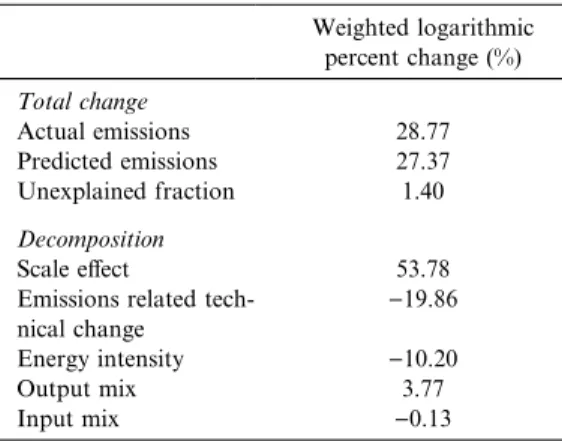
random error term. The contributions of the five effects to changes in global emissions at the global level are given in Table 3. Input and output effects contributed little globally, though in individual countries they can have important effects. At the global level the two forms of technological change reduced the increase in emissions to half of what it would have been in their absence with emissions spe-cific technological change lowering aggregate emissions by around 20%. The residuals from the model show it to be a statistically adequate

representation of the data. A nested test of this model and the EKC showed that the income squared term in the EKC added no explanatory power to that provided by the decomposition model.

In an attempt to determine the effects of trade on scale, composition, and technique effects, Antweiler et al. (2001) estimate a dif-ferent type of econometric decomposition model that derives a reduced form equation from a theoretical structural model of the demand and supply of pollution. The technique effect is however assumed to be induced by the increase in income due to trade. This model, therefore, takes the EKC hypothesis as a given. The composition effect is expected to differ in capital intensive and labor intensive economies. Trade is likely to increase pollution in the former and reduce it in the latter. Therefore, the capital/labor ratio is controlled for. The model is estimated using the GEMS sulfur dioxide concentration data. Rather than a decomposition of changes in emissions they compute elasticities with respect to the different factors. The ‘‘scale elasticity’’ is estimated to average 0.266. The sample mean of the tech-nique elasticity (elasticity of concentrations w.r.t. GNP per capita) is)1.15. The composi-tion elasticity (elasticity of concentracomposi-tions w.r.t. capital/labor ratio) is 1.01 and trade intensity has an elasticity of )0.864. Combining the effects, trade has a negative impact on emis-sions. Cole and Elliott (2003) extend the anal-ysis to other pollutants and to emissions. The results are more mixed.

The conclusion from all these studies is that the main means by which emissions of pollu-tants can be reduced is by time related tech-nique effects and in particular those directed specifically at emissions reduction, though productivity growth or declining energy inten-sity has a role to play. Though structural change and shifts in fuel composition may be important in some countries at some times, their average contribution seems less important quantitatively. Those studies that include developing countries (e.g., Antweiler et al., 2001; Judsonet al., 1999; Stern, 2002) find that these technological changes are occurring in both developing and developed countries. Innovations may first be adopted preferentially in higher income countries (Hilton & Levinson, 1998) but seem to be adopted in developing countries with relatively short lags (Gallagher, 2003). This result is in line with the evidence of Dasgupta et al. (2002) and the EKC-based

Table 3. Contributions to total change in global sulfur emissions Weighted logarithmic percent change (%) Total change Actual emissions 28.77 Predicted emissions 27.37 Unexplained fraction 1.40 Decomposition Scale eﬀect 53.78

Emissions related tech-nical change

)19.86 Energy intensity )10.20

Output mix 3.77

(17)

estimates of time eﬀects in Stern and Common (2001) and Stern (2002).

9. CONCLUSIONS

The evidence presented in this paper shows that the statistical analysis on which the envi-ronmental Kuznets curve is based is not robust. There is little evidence for a common inverted U-shaped pathway that countries follow as their income rises. There may be an inverted U-shaped relation between urban ambient con-centrations of some pollutants and income though this should be tested with more rigorous time-series or panel data methods. It seems unlikely that the EKC is an adequate model of emissions or concentrations. I concur with Copeland and Taylor (2004), who state that: ‘‘Our review of both the theoretical and empirical work on the EKC leads us to be skeptical about the existence of a simple and predictable relationship between pollution and per capita income.’’

The true form of the emissions–income rela-tionship is likely a mix of two of the scenarios proposed by Dasgupta et al. (2002) illustrated in Figure 3. The overall shape is that of their ‘‘new toxics’’ EKC––a monotonic increase of emissions in income. But over time this curve shifts down, which is analogous to their ‘‘revised EKC’’ scenario. Some evidence shows that a particular innovation is likely to be adopted preferentially in high-income countries

first with a short lag before it is adopted in the majority of poorer countries. However, emis-sions may be declining simultaneously in low-and high-income countries over time, ceteris paribus, though the particular innovations typically adopted at any one time could be different in different countries.

It seems that structural factors on both the input and output side do play a role in modi-fying the gross scale effect though they are mostly less influential than time-related effects. The income elasticity of emissions is likely to be less than one––but not negative in wealthy countries as proposed by the EKC hypothesis. In slower growing economies, emissions-reducing technological change can overcome the scale effect of rising income per capita on emissions. As a result, substantial reductions in sulfur emissions per capita have been observed in many OECD countries in the last few decades. In faster growing middle income economies, the effects of rising income over-whelmed the contribution of technological change in reducing emissions.

The research challenge now is to revisit some of the issues addressed earlier in the EKC lit-erature using the new decomposition and frontier models and rigorous panel data and time-series statistics. For example, how can the eﬀects of trade on emissions be modeled in the context of the decomposition and econometric frontier models?15 _{Rigorous answers to such}

questions are central to the debate on global-ization and the environment.

NOTES

1. The increasing number of exceptions include Cole (2003b), Coondoo and Dinda (2002), Day and Grafton (2003), de Bruyn (2000), Stern and Common (2001), Perman and Stern (2003), Friedl and Getzner (2003), and Heil and Selden (1999, 2001).

2. Exceptions include Stern and Common (2001) and Magnani (2001).

3. For example: Dasgupta et al. (2002), Harbaugh, Levinson, and Wilson (2002), Perman and Stern (2003), and Koop and Tole (1999).

4. Kander (2002) argues that structural shift in the economy may largely be an illusion. Due to rising productivity in manufacturing, manufacturing prices fall

relative to the prices of services and therefore manufac-turing’s share of GDP declines when measured at current prices but not when measured at constant prices. Due to this productivity growth in manufacturing, its pollution intensity falls over time relative to the pollu-tion intensity of services.

5. Grossman (1995) calls the combination of 3 and 4 the ‘‘technique eﬀect.’’

6. Later published as Grossman and Krueger (1994). 7. Later published as Shaﬁk (1994).

8. Also see Ezzati, Singer, and Kammen (2001).

(18)

9. Solid waste does not necessarily result in ‘‘pollu-tion,’’ especially as techniques to reduce seepage and emissions from landﬁlls and increase recycling have progressed. But landﬁlls still disturb the landscape and geology and recycling and waste processing require additional energy and resource use.

10. See the discussion of energy EKCs above. 11. In an alternative test for omitted variables, Mag-nani (2001) uses the Ramsey test on cross-sectional EKCs and ﬁnds that the null of no omitted variables is rejected in almost every case.

12. Judson, Schmalensee, and Stoker (1999) estimate separate EKC relations for energy consumption in each of a number of energy-consuming sectors for a large panel data set using spline regression, which allows them to estimate diﬀerent time eﬀects in each sector. These vary substantially energy consumption rises over time,

ceteris paribus, in the household and other sectors but

are ﬂat to declining in industry and construction. Technical innovations tend to introduce more energy using appliances to households and energy saving techniques to industry.

13. Judsonet al. (1999) decompose emissions by sector and then ﬁt EKC models––see the previous endnote. 14. Lansink and Silva (2003), Reinhardet al. (1999), and Fernandezet al. (2002) all look at agricultural ﬁrms rather than countries.

15. Bruvollet al. (2003) provide a possible method for a single country model. But they only investigate emissions directly associated with imports and exports and not the effects of trade on the overall pollution intensity of the economy. Antweileret al. (2001) and Cole and Elliott (2003) provide another approach with different limitations––for example, the technique effect is assumed to be induced by an EKC like income effect.

REFERENCES

Andreoni, J., & Levinson, A. (2001). The simple analytics of the environmental Kuznets curve. Jour-nal of Public Economics, 80, 269–286.

Ansuategi, A., & Perrings, C. A. (2000). Transboundary externalities in the environmental transition hypoth-esis.Environmental and Resource Economics, 17, 353– 373.

Ansuategi, A., Barbier, E. B., & Perrings, C. A. (1998). The environmental Kuznets curve. In J. C. J. M. van den Bergh & M. W. Hofkes (Eds.), Theory and implementation of economic models for sustainable development. Dordrecht: Kluwer.

Antweiler, W., Copeland, B. R., & Taylor, M. S. (2001). Is free trade good for the environment. American Economic Review, 91, 877–908.

Arrow, K., Bolin, B., Costanza, R., Dasgupta, P., Folke, C., Holling, C. S., Jansson, B.-O., Levin, S., M€aler, K.-G., Perrings, C. A., & Pimentel, D. (1995). Economic growth, carrying capacity, and the envi-ronment.Science, 268, 520–521.

Beckerman, W. (1992). Economic growth and the environment: Whose growth? Whose environment?

World Development, 20, 481–496.

Bruvoll, A., & Medin, H. (2003). Factors behind the environmental Kuznets curve: A decomposition of the changes in air pollution. Environmental and Resource Economics, 24, 27–48.

Bruvoll, A., Fæhn, T., & Strøm, B. (2003). Quantifying central hypotheses on environmental kuznets curves for a rich economy: A computable general equilib-rium study. Scottish Journal of Political Economy, 50(2), 149–173.

Bulte, E. H., & van Soest, D. P. (2001). Environmental degradation in developing countries: Households

and the (reverse) environmental Kuznets Curve.

Journal of Development Economics, 65, 225–235. Cole, M. A. (2003a). Environmental optimists,

environ-mental pessimists and the real state of the world––an article examining The Skeptical Environmentalist: Measuring the Real State of the World by Bjorn Lomborg.Economic Journal, 113, 362–380. Cole, M. A. (2003b). Development, trade, and the

environment: How robust is the environmental Kuznets curve? Environment and Development Eco-nomics, 8, 557–580.

Cole, M. A., Elliott, R. J., & R (2003). Determining the trade–environment composition eﬀect: The role of capital, labor and environmental regulations.Journal of Environmental Economics and Management, 46, 363–383.

Cole, M. A., Rayner, A. J., & Bates, J. M. (1997). The environmental Kuznets curve: An empirical analysis.

Environment and Development Economics, 2(4), 401– 416.

Coondoo, D., & Dinda, S. (2002). Causality between income and emission: A country group-speciﬁc econometric analysis. Ecological Economics, 40, 351–367.

Copeland, B. R., & Taylor, M. S. (2004). Trade, growth and the environment. Journal of Economic Litera-ture, 42, 7–71.

Dasgupta, S., Laplante, B., Wang, H., & Wheeler, D. (2002). Confronting the environmental Kuznets curve.Journal of Economic Perspectives, 16, 147–168. Day, K. M., & Grafton, R. Q. (2003). Growth and the environment in Canada: An empirical analysis.

Canadian Journal of Agricultural Economics, 51, 197–216.