Advances in Mechanical Engineering 2020, Vol. 12(12) 1–13 ÓThe Author(s) 2020 DOI: 10.1177/1687814020975544 journals.sagepub.com/home/ade
Optimization of the setup position of a
workpiece for five-axis machining to
reduce machining time
Ching-chih Wei
and Wei-chen Lee
Abstract
Five-axis machining is commonly used for complicated features due to its advantage of rotary movement. However, the rotary movement introduces nonlinear terms in the kinematic transform. The nonlinear terms are related to the dis-tance between the cutter location (CL) data and the intersection of the two rotary axes. This research studied the possi-ble setup positions after the toolpaths have been generated, and the objective was to determine the optimal setup position of a workpiece with minimal axial movements to reduce the machining time. We derived the kinematic trans-form for each type of five-axis machines, and then, defined an optimization problem that described the relationship between the workpiece setup position and the pseudo-distance of the axial movements. Eventually, an optimization algo-rithm was proposed to search for the optimal workpiece setup position within the machinable domain, which is already concerned with over-traveling and machine interference problems. In the end, we verified the optimal results with a case study with a channel feature, which was real cutting on a table-table type five-axis machine. The results show that we can save the axial movements up to 16.76% and the machining time up to 10.70% by setting up the part at the optimal position.
Keywords
Five-axis machining, optimization, workpiece setup position, minimal axial movement, machining time reduction
Date received: 20 February 2020; accepted: 14 September 2020 Handling Editor: James Baldwin
Introduction
Background
In general, a five-axis machine is constructed with three linear axes and two rotary axes, with which the cutting tool can be tilted to cut free-form surfaces and avoid collision between the tool and the workpiece. In addi-tion, the workpiece can be fabricated within minimum setup times, which can effectively reduce machining time including the time for planning multiple setups and making customized fixtures. Although the five-axis machining has the advantages mentioned above, it still requires operators to make many decisions, such as tool selection, tool orientation, and setup position, which may affect the machining efficiency.
Usually, engineers could directly generate the five-axis toolpaths for a part using CAM software. The toolpaths represent the tooltip position and the tool orientation, based on the workpiece coordinate system (WCS). Nevertheless, the machine only recognizes the position relative to the machine coordinate system (MCS). Thus, a transformation between the WCS and Department of Mechanical Engineering, National Taiwan University of Science and Technology, Taipei City
Corresponding author:
Wei-chen Lee, Department of Mechanical Engineering, National Taiwan University of Science and Technology, No.43, Keelung Rd., Sec.4, Da’an Dist., Taipei 10607.
Email: [email protected]
Creative Commons CC BY: This article is distributed under the terms of the Creative Commons Attribution 4.0 License (https://creativecommons.org/licenses/by/4.0/) which permits any use, reproduction and distribution of the work without further permission provided the original work is attributed as specified on the SAGE and Open Access pages
the MCS is necessary. During the process, the tool tra-jectory is complex due to the motion caused by the two rotary movements. Moreover, due to the varying dis-tance between the tooltip position and the rotary center, different setup positions can cause different tool trajec-tories in MCS. In other words, machining efficiency can be improved by optimizing the setup position of a workpiece. Until now, the decision for a setup position still depends on the operator’s experience. The experi-ence cannot guarantee that the two major issues will not occur: one is the collision between the tool assembly and the machine components, and the other is over-traveling occurring on the linear axes. Additionally, lit-tle research on the relationship between the setup posi-tion and the machining efficiency has been made.
Literature review
In general, cutter location (CL) data is used to describe the toolpaths. The CL data have to be transformed to the NC code, which is based on the MCS, so that the machine can move accordingly. Thus, the kinematic transforms for five-axis machine structures are needed. Five-axis machine are commonly categorized into three types: head-head, head-table, and table-table, based on the location of the two rotary axes. Many researchers have studied kinematics of the machines using the homogeneous coordinate transformation matrices in Denavit-Hartenberg notation.1 Lee and She2 derived kinematics for a head-head type, a head-table type, and a table-table type. Jung et al.3developed a postproces-sor for a table-table five-axis machine tool with A and C axes (TATC), and then proposed an algorithm to prevent interference in certain situations. She and Lee4 and She and Chang5designed a generalized kinematic model, which combines the primary and the secondary rotary axes on both the spindle side and the table side. The generalized kinematic model can be applied to all types of five-axis machine tools. Sørby6derived forward and inverse kinematics for five-axis machine tools with non-orthogonal rotary axes B and C on the worktable. Yang and Altintas7used the screw theory to develop a generalized forward and inverse kinematic transform method, which models each kinematic element as a revolute joint or prismatic joint. The screw theory method can easily calculate the inverse kinematics with only the point and vector of each joint. Many research-ers developed kinematic models containing nonlinear terms due to the involvement of two rotary axes. The nonlinear terms result in variations of distance equation within five-axis machining trajectories. The result of distance equation could be altered in two aspects, as discussed in the following. One is the orientation of the workpiece; the other is the position of the workpiece. However, the two factors are too complicated to be considered at the same time. Some researchers studied
the effects of the orientation of a workpiece on planning the toolpath. Lee et al.8determined the optimal work-piece orientation by the minimum rotary movement. Hu et al.9determined the optimal setup by the largest intersection of the visibility maps. Some researchers studied the position of the workpiece after the toolpath had been defined. Anotaipaiboon et al.10 studied the optimization problem of the workpiece position to minimize the kinematic errors caused by nonlinear tool trajectory. Tutunea-Fatan and Bhuiya11 proposed a method to determine the nonlinear errors of the head-head type five-axis machine. Then, they compared the efficiency between the structures with different combi-nations of rotary axes, and found that the combination with vertical rotational axis tends to move more than with only horizontal rotational axes. Lin et al.12focused on the movement errors on a TATC type machine. Then, the optimal workpiece position was found by using particle swarm optimization in the machinable domain to minimize the nonlinear error caused by the rotary movement. The machinable domain was con-structed as a cuboid field according to the travel of three linear axes of machine. Xu and Tang13considered energy efficiency on the movement of each axis. Then, they proposed an algorithm to find the optimal work-piece setup with minimum energy cost. Shaw and Ou14 derived a transformation matrix on a TATC type machine to find the minimum movement on the X, Y, and Z axes. Then, he used a generic algorithm to search for the best position for the workpiece in a cuboid domain that formed with a limit of three linear axes. Pessoles et al.15defined the pseudo-distance as a sum of the maximum movement for the three linear axes along the toolpaths. He discretized the possible domain of a workpiece setup position, and then he computed the pseudo-distances for all the setup positions. Eventually, the optimal workpiece setup position was determined by finding the minimum pseudo-distance.
Objective
The research above studied about the machining dis-tance of table-table type machines with AC type and BC type configurations. Nevertheless, the relationship between the workpiece position and the machining time is still unknown for different types of five-axis machines. The machining time is a complicated issue affected by system performance, including toolpath tra-jectory complexity, acceleration planning, and motor response. To simplify the problem, we considered the axial movement distance as a measure of the machining time and ignored all the other factors that may affect the machining time. In addition, over-traveling and interference problems between the tool assembly and the machine components have not been considered yet. In other words, the workpiece may not be completed
due to over-traveling or interference problems. Therefore, the objective of this research was to deter-mine the optimal setup position of a workpiece with minimal axial movements on a tool trajectory in a machinable domain, where the workpiece can be machined with one setup without problems including over-traveling of each axis or interference between the tool assembly and the machine components.
Statement of the optimization problem
Kinematics of a five-axis machine
16In this section, we only derived the kinematic transform of A and C rotary axes for each type of the machines. Likewise, the machine with different rotary axes can be derived. To derive the kinematic model for each type of five-axis machine, we have to use six coordinate sys-tems: WCS (OWXYZ) and MCS (OMXYZ) and the other four are defined as follows.
(1) The coordinate system at the fourth rotary cen-ter (O4XYZ), which is the center of the primary rotary axis.
(2) The coordinate system at the fifth rotary center (O5XYZ), which is the center of the second rotary axis.
(3) The spindle-nose coordinate system (SCS, OSXYZ), which is located at the center of the spindle-nose.
(4) The tool coordinate system (TCS, OTXYZ), which is located at the controlled cutting point on the tool. The cutting point can be either the tooltip or the tool center.
The relationship between the six coordinate systems in a TATC type, which means the fourth axis is an A axis, and the fifth axis is a C axis on a table-table type five-axis machine, can be illustrated in Figure 1. As shown in the figure, dM!S represents the vector from OMXYZ to OSXYZ; dS!T represents the vector from OSXYZ to OTXYZ; dM!4th represents the vector
from OMXYZ to O4XYZ;d4th!5th represents the vector
from O4XYZ to O5XYZ; d5th!W represents the
vector from O5XYZ to OWXYZ.
The CL data can be transformed from OWXYZ to OMXYZ in five steps. The overall transformation matrix on the table side can be obtained through the five steps described below:
(1) Translate from OWXYZ to O5XYZ with vector
d5th!W.
(2) Rotate an angle C around the C axis in O5XYZ.
(3) Translate from O5XYZ to O4XYZ with vector
d4th!5th.
(4) Rotate an angle A around the A axis in O4XYZ.
(5) Translate from O4XYZ to OMXYZ with vector
dM!4th.
We defineTrans(d) as a translation transformation matrix with vectord, andRotX(A),RotY(B), RotZ(C) as a rotary transformation matrix with A, B and C
angles rotated around the X, Y, and Z axes, respec-tively. In this case, the rotary axis is placed on the table side. Since the direction of rotary movement is defined by the tool, the rotary direction is opposite when the rotary axis is on the table side. After all the transforma-tions are performed, the cutter location can be repre-sented in OMXYZ. To coincide the controlled cutting point on the tool to the cutter location in terms of the MCS, we need to transform the position of the cutting point from OTXYZ to OMXYZ. The transformation matrix of the spindle side, which is denoted by the matrix S, can be derived in two steps: (1) Translate from OSXYZ to OTXYZ with vectort, which is defined as the vector from the cutting location on the tool to the spindle-nose. (2) Translate from OMXYZ to OSXYZ with vector dM!S. Thus, the two transforma-tion matrices of the TATC machine are defined as equations (1) and (2).
(1) TATC type
T=Trans(dM!4th)RotX(A)Trans(d4th!5th) RotZ(C)Trans(d5th!W)
ð1Þ
S=Trans(dM!S)Trans(dS!T) ð2Þ Similarly, the relationship between each coordinate system of the head-table type and head-head type, or the
Figure 1. (a) Coordinate systems defined on the table-table type five-axis machine and (b) their relationship.
HATC type and the HCHA type, five-axis machine can be illustrated in Figures 2 and 3, respectively. The trans-formation of these two types of machines can be derived by using the kinematic chain loop as well. The transfor-mation matrices are defined as equations (3) to (6).
(2) HATC type
T=Trans(dM!5th)RotZ(C)Trans(d5th!W) ð3Þ
S=Trans(dM!4th)RotX(A)Trans(d4th!S)Trans(dS!T)
ð4Þ
(3) HCHA type
T=Trans(dM!W) ð5Þ
S=Trans(dM!4th)RotZ(C)Trans(d4th!5th) RotX(A)Trans(d5th!S)Trans(dS!T)
ð6Þ
Define the optimization problem of the workpiece
position with axial movements
The five-axis toolpath generated in CAM software usu-ally consists of small linear segments. To keep the tool-tip on the toolpath, we need to obtain the transformation matrices derived in section 2.1. As shown in Figure 4(a), the toolpath is a linear path in OWXYZ (solid line). The linear path can be divided into small segments by time interpolation, and then, the position of each segment can be transformed into OMXYZ to form the true trajectory in Figure 4(b)
(dotted line) as a nonlinear movement. The started position and ended position of the nonlinear movement are shown in Figure 4(b) and (c), respectively. Here, the nonlinear movement caused by rotary axes would introduce nonlinear terms in the kinematic transform.
As shown in Figure 4(d), we define an offset vector
dw to shift the WCS from OWXYZ to OW1XYZ. Although the toolpath relative to OW1XYZ stays the same as shown in Figure 4(e), the true trajectory rela-tive to OMXYZ is altered due to the change of the workpiece setup position OWXYZ. With the new work-piece setup position, The started position and ended position of the true trajectory are shown in Figure 4(f), which is different from those in Figure 4(c). Next, we derived the relationship between the offset dw and the total axial movements on the true trajectory, to deter-mine the setup position with the shortest axial movements.
Because the linear and rotary movements in a single NC block would be completed simultaneously, we used the pseudo-distance instead of the linear distance to represent the total axial movements. Typically, the total pseudo-distance,17 which will be called distance in the following, of the axial movements is determined as the root sum square of the movement in each axis, as shown in equation (7), in whichlis defined as the total pseudo-distance of the whole trajectory, and li is defined as the distance on segment i of the trajectory. (Xi1,Yi1,Zi1,Ai1,Ci1) and (Xi,Yi,Zi,Ai,Ci) stand for the start and end positions of each axis in segmenti
defined in OMXYZ, respectively. l=X n i=1 ffiffiffiffiffiffiffiffiffiffiffiffiffiffiffiffiffiffiffiffiffiffiffiffiffiffiffiffiffiffiffiffiffiffiffiffiffiffiffiffiffiffiffiffiffiffiffiffiffiffiffiffiffiffiffiffiffiffiffiffiffiffiffiffiffiffiffiffiffiffiffiffiffiffiffiffiffiffiffiffiffiffiffiffiffiffiffiffiffiffiffiffiffiffiffiffiffiffiffiffiffiffiffiffiffiffiffiffiffiffiffiffiffiffiffiffiffiffiffiffiffiffiffiffiffiffiffiffiffiffiffiffiffiffiffiffiffiffiffiffiffiffiffi (XiXi1)2+ (YiYi1)2+ (ZiZi1)2+ (AiAi1)2+ (CiCi1)2 q = X n i=1 li ð7Þ
Figure 2. (a) Coordinate systems defined on the head-table
type five-axis machine and (b) their relationship. Figure 3. (a) Coordinate systems defined on the head-head type five-axis machine and (b) their relationship.
To find the pseudo-distance, first, we derived the 4 4 homogeneous transformation matrixTi and Si with different kinematics of machine with the rotary angles AandC according to the steps in section 2.1. The gen-eral form of the transformation matrices can be repre-sented as equations (8) and (9). We defined 3 3 matrices,RTi andRSi, as the rotary matrices, and 3 1 matrices,LTi andLSi, as the translation matrices inTi andSi, respectively. Then, the CL data in OWXYZ can be transformed into the tool position in OMXYZ with equation (10), defined as pi. (xi,yi,zi) and (Xi,Yi,Zi) represent the coordinates in OWXYZ and OMXYZ, respectively, in the toolpath segmenti.
Ti= RTi333 LTi331 0133 1 ð8Þ Si= RSi333 LSi331 0133 1 ð9Þ pi= Xi Yi Zi 1 0 B B @ 1 C C A=Ti xi yi zi 1 0 B B @ 1 C C ASi 0 0 0 1 0 B B @ 1 C C A ð10Þ
We can define an offset vector (p,q,r) as the move-ment from the original setup position. As shown in equation (11), the position of the start position of seg-ment i can be transformed into the machine position with the offset of the setup position. Since the addi-tional offset vector (p,q,r) is a 3 1 vector, we need to add an element 0 to make it a homogeneous coordinate. pi ð Þoffset=Ti xi yi zi 1 0 B B B @ 1 C C C A+ p q r 0 0 B B B @ 1 C C C A 0 B B B @ 1 C C C ASi 0 0 0 1 0 B B B @ 1 C C C A =pi+ RTi333 LTi331 0133 1 p q r 0 0 B B B @ 1 C C C A ð11Þ
Because the fourth element of homogeneous coordinate is used for homogeneous transformation only, we can reduce the vectorð Þpi offsetfrom 4 1 to 3 1, as shown in equation (12). Then the start and end positions of seg-ment i can be transformed to the machine positions
Figur 4. Calculating from a five-axis toolpath in OWXYZ (solid line) to a true trajectory in OMXYZ (dotted line): (a) Original workpiece setup position with five-axis toolpath, (b) tool started position in the true trajectory, (c) tool ended position in the true trajectory, (d) new workpiece setup position OW1XYZ with offsetdw, (e) new workpiece setup position with five-axis toolpath and
with the consideration of the offset of the setup posi-tion, as shown in equations (12) and (13).
pi ð Þoffset= Xi Yi Zi 0 @ 1 A offset =pi+RTi p q r 0 @ 1 A ð12Þ pi1 ð Þoffset= Xi1 Yi1 Zi1 0 @ 1 A offset =pi1+RTi1 p q r 0 @ 1 A ð13Þ
Here we defined DXi,DYi, andDZi as the following equation by subtracting equation (13) from equation (12), DXi DYi DZi 0 B @ 1 C A offset = Xi Yi Zi 0 B @ 1 C A offset Xi1 Yi1 Zi1 0 B @ 1 C A offset = (pipi1) + (RTiRTi1) p q r 0 B @ 1 C A ð14Þ
In addition, we definedDAi andDCias the movements of two rotary axes in segment i, as shown in equations (15) and (16). Thus, the pseudo-distance of segmenti, li, can be calculated by using equation (17), with the con-sideration of the offset of the setup position.
DAi=AiAi1 ð15Þ DCi=CiCi1 ð16Þ li= ffiffiffiffiffiffiffiffiffiffiffiffiffiffiffiffiffiffiffiffiffiffiffiffiffiffiffiffiffiffiffiffiffiffiffiffiffiffiffiffiffiffiffiffiffiffiffiffiffiffiffiffiffiffiffiffiffiffiffiffiffiffiffiffiffiffiffiffiffiffiffiffi DXi2+DYi2+DZi2+DAi2+DCi2 q ð17Þ
As shown in equation (17), it is well-known that the Euclidean distance is a convex function.18 In other words, the equation is a typical convex function, we called the distance functionf. However, the domain of the distance functionf,F, is different from the machin-able domain which exists the offset vector (p,q,r), which is denoted byG. Thus, the mapping fromFtoG
is needed.
Since the rotary movements stay the same within the transformation from OWXYZ to OMXYZ, the terms
DAi andDCi are constant. Therefore, the terms would not affect the convexity of the distance function. Thus, we can simplify the equation by eliminating the terms
DAiandDCifrom equation (17). The simplied vector is denoted byLi,
Li=ðDXi,DYi,DZiÞ ð18Þ Then we can redefine the distance function of segment
i,li, which is the Euclidean norm ofLi, li=
ffiffiffiffiffiffiffiffiffiffiffiffiffiffiffiffiffiffiffiffiffiffiffiffiffiffiffiffiffiffiffiffiffiffiffiffiffiffiffiffi DXi2+DYi2+DZi2
p
=k kLi =f(Li) ð19Þ
The vectorLican be represented as equation (20) from equation (14) with an affine mapping,
Li= DXi DYi DZi 0 B @ 1 C A= (RTiRTi1) p q r 0 B @ 1 C A + (pipi1) =Mdw+N ð20Þ
whereRTi1andRTi are the rotary matrices in the
trans-formation relative to the start positionpi1and the end position pi, respectively. M is the matrix obtained by subtracting RTi1 from RTi, which is a linear
transfor-mation in the machinable domainG. The vector dw is the offset vector (p,q,r) in G. N is a vector in the domainF.
The distance function now is f:R3!R,M2R333, andN2R3, then we can define the functiong:R3!R
by
g(dw) =f(Mdw+N) =f(Li) ð21Þ which maps the distance functionf from the domainF
to the domainG. We can defineu,v2R3in the domain of the functiong. Then8l2 ½0, 1,
g(lu+ (1l)v) =f(M(lu+ (1l)v) +N) =f(l(Mu+N) + (1l)(Mv+N)) łf(l(Mu+N)) +f((1l)(Mv+N)) =lf(Mu+N) + (1l)f(Mv+N) =lg(u) + (1l)g(v) ð22Þ
The equation shows that the function g is a convex function as well. Then, the objective function, which is the total distancel, can be represented as
l=X n i=1 li= Xn i=1 g(dw) ð23Þ
The objective function,l, is a non-negative weighted sum of convex functions. We can define non-negative weightsa,b ø0andg1,g2 as convex function. Follow
the definition of a convex function,8l2 ½0, 1,
g1(lu+ (1l)v)ł lg1(u) + (1l)g1(v) ð24Þ g2(lu+ (1l)v)ł lg2(u) + (1l)g2(v) ð25Þ Then,8l2 ½0, 1, h(lu+ (1l)v) =ag1(lu+ (1l)v) +bg2(lu+ (1l)v) ł a(lg1(u) + (1l)g1(v)) +b(lg2(u) + (1l)g2(v)) =lh(u) + (1l)h(v) ð26Þ
where h=ag1+bg2, which can be proved as a
convex function. With the proof above, the objective function,l, is a convex function in machinable domain
G. In other words, there exists a global minimum that is the same as the local minimum in the set oflnwith a spatial set of setup offset variablesdw. The objective of the optimization problem is to determine the optimal setup position of the workpiece to minimize the total distance for the axial movements in the machinable domain, minimize dw l=X n i=1 li= Xn i=1 g(dw)
subject to the offset vectordwin the machinable domainG
ð27Þ
Next, we proposed an algorithm to search the optimal result within the constraint region of the machinable domain.19
Method to determine the optimal setup
position
The objective function has been proven as a convex function, which means that the local minimum is the same as the global minimum in a dexel. Hence, we can use the gradient descent method to search for the mini-mum in the machinable domain for each dexel.20 The machinable domain is the collection of all possible setup position without having problems including over travel limits of any linear axis and collision between the tool assembly and the machine components. However, the machinable domain is too complicated so that
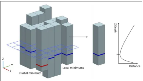
practically it can be described in discretized dexel, which is pixels on the XY plane with depth information in the Z-axis, as shown in Figure 5.
To ensure that the global minimum is selected within the machinable domain, we need to check each local minimum to obtain the global minimum. The local min-imum is the minmin-imum in each dexel. Nevertheless, there might exist certain minimal values that are the same as the global minimum. Thus, we proposed another criter-ion to select the global minimum from the same mini-mum values at different positions. The criterion is to choose the position closest to the center of the workta-ble in order to meet the common setting in industry. Eventually, the optimal workpiece setup position with the shortest distance of the axial movements can be obtained.
As a result of optimization,doptrefers to the shortest total axial movements with the workpiece in the opti-mal setup position. dorg refers to the original distance of the workpiece in the original setup position. In gen-eral, the original setup position is set at the center of the pallet table. To comparedopt withdorg,dR is defined in equation (28) as a percentage of reduced axial move-ments. Moreover, the optimized and original machin-ing timetoptandtorgare recorded in the case study.tR is defined as the percentage of the reduced machining time, as shown in equation (29).
dR= dorgdopt dorg 3100% ð28Þ tR= torgtopt torg 3100% ð29Þ
Figure 5. Represent domain with discretized dexels. Each dexel has one local minimum (blue layer), then compare and select the minimal value as a global minimum in the domain (red layer).
Experimental environment and setup
Experimental environment
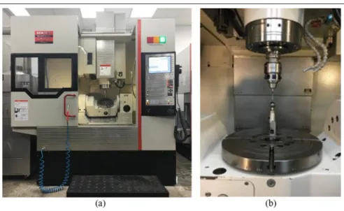
In this research, the toolpaths would be planned in NX software (Siemens, Germany) and then simulated on a TATC machine (Model Number UX300, Quaser, Taiwan), as shown in Figure 6(a), which is equipped with a Heidenhain iTNC530 controller. The specifica-tions of the machine, including the travel limit (Table 1) and the offset data of the coordinate system (Table 2), were applied to calculate the optimal workpiece setup position. The offset data from O5XYZ to OwXYZ was set to zero because we coincided these two points with the setup setting on machine. The dimensions of the five-axis machinedM!4th andd4th!5th were measured by using the Heidenhain probe TS740 and the Heidenhain calibration sphere KKH100 with the CYCLE451 com-mand built in the Heidenhain controller, as shown in Figure 6(b). After that, we machined the parts to obtain the cutting time for comparison among different work-piece setup positions.
Example of optimization program process
In this section, we would use a simple example to demonstrate the process of optimization. The example
is a linear cutting toolpath. The CL data are shown as follows,
FEDRAT/MMPM, 1000.0000
GOTO/0.000, 0.000, 0.000, 0.000, 0.000 GOTO/10.000, 20.000, 30.000, –40.000, 50.000 The start position (x1,y1,z1,A1,C1) is (0,0,0,08,08), and the end position (x2,y2,z2,A2,C2) is (10,20,30,408,508) defined in OWXYZ. The unit of the linear axes X, Y, and Z was millimeter, and that of the rotary axes A and C was degree. The length of the cutting toolpathdcutwas 37.4166 mm, which was calcu-lated as a root sum square distance from (0,0,0) to (10,20,30), dcut= ffiffiffiffiffiffiffiffiffiffiffiffiffiffiffiffiffiffiffiffiffiffiffiffiffiffiffiffiffiffiffiffiffiffiffiffiffiffiffiffiffiffiffiffiffiffiffiffiffiffiffiffiffiffiffiffiffiffiffiffiffiffiffiffiffiffiffiffiffiffi (x2x1)2+ (y2y1)2+ (z2z1)2 q =37:4166 ð30Þ
The first step was to divide the toolpath into small seg-ments with the interpolation time of the controllertipt, which was 0.1 ms for the iTNC530 controller. Because the feed rate Fin the CL data was 1000 mm/min, the interpolation distancediptwas calculated as follow,
Figure 6. (a) Quaser UX300 five-axis machine with a Heidenhain controller. (b) Measuring the machine kinematics by a Heidenhain probe TS740 and a calibration sphere KKH100.
Table 1. Quaser UX300 axis limits.
Machine travel Negative limit Positive limit
X 2205 mm 205 mm
Y 2305 mm 305 mm
Z 2500 mm 0 mm
A 2120° 30°
C 360°continuous
Table 2. Offset data measured from the machine. Coordinate system Offset data (mm) OMXYZ to O4XYZ (dM!4th) X 0.0000 Y 20.0012 Z 2529.8644 O4XYZ to O5XYZ (d4th!5th) X 20.0370 Y 20.0164 Z 20.0224
dipt=Ftipt=60000 =0:0017 ð31Þ Then we can extract the first segment of the cutting path by usingript, the ratio of the interpolation distance dipt and the length of the cutting toolpathdcut. In this example,
ript=dipt=dcut=0:0017=37:4166=4:54343105: ð32Þ
With the interpolation ratio ript, the interpolated lengths or angles can be calculated as (0:4543,0:9087, 1:3630, 1:81748,2:27178)3103 between the start position and the end position along the five axes of the machine tool.
Next, we focused on the interpolation segment between position A (0,0,0,08,08) and position B(0:4543,0:9087, 1:3630, 1:81748,2:27178)3103. The transformation matrices related to both positions can be calculated as follows by using equations (1) and (2). Here we substitute coordinate of position A and B, the kinematics data in Table 2 into the transformation matrices, and the cutting tool we used is 100.125 mm measured from the spindle nose to the tooltip along the –Z direction. TA= 1 0 0 0:0370 0 1 0 0:0176 0 0 1 529:8868 0 0 0 1 0 B B @ 1 C C A ð33Þ SA= 1 0 0 0 0 1 0 0 0 0 1 100:125 0 0 0 1 0 B B @ 1 C C A ð34Þ TB= 1 3:96493105 0 0:0370 3:96493105 1 3:17203105 0:0176 1:25763109 3:17203105 1 529:8868 0 0 0 1 0 B B @ 1 C C A ð35Þ SB= 1 0 0 0 0 1 0 0 0 0 1 100:125 0 0 0 1 0 B B @ 1 C C A ð36Þ
With the elements in the transformation matrices, we can use equation (17) to obtain the distance function of segment one as li= (1:57203109p2+2:57813109q2 +1:00613109r2 3:989231014pq+2:51533109pr +4:986431014qr 7:21113108p+1:22463107q 5:76893108r+1:13533105)1=2 ð37Þ
Then we can derive the gradient of the distance func-tion of segment one as the partial derivative of the dis-tance function with respect tor, which is the offset of the workpiece setup position along the Z-axis, as shown in equation (38). After adding all of the gradients, we can obtain the total gradient as equation (39).
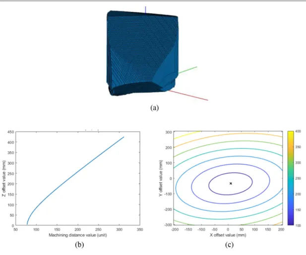
∂li ∂r = (1:00613109r+2:51533109p+4:986431014q5:76893108) 2li ð38Þ g=X n i = 1 ∂li ∂r ð39Þ With the numerical gradientg, we can calculate the optimal valuer by using the gradient descent method in each dexel. For instance the dexel atxandyposition (0,0), the gradient is calculated by substitutep=q= 0 into equation (39). The range ofrat the (0,0) position was [4,425] along the Z-axis, which was obtained from the machinable domain as shown in Figure 7(a). The machinable domain is calculated by the algorithm we proposed.19 Thus, the local minimum value can be obtained at 4 mm offset along the Z-axis on the dexel at (0,0) position, as shown in Figure 7(b), where the relationship between the machining distance and the offset value is illustrated. After the optimization pro-gram computed the minimum for each dexel, the global minimum value was found at (10,35) with the opti-mal offset value 4 mm along the Z-axis, which is the
position of the minimum value shown in the contour plot of Figure 7(c).
Case study
A cuboid with a curved channel was used to demon-strate our study, as shown in Figure 8(a). The channel
is altered from 30 mm to 28 mm in diameter along a spline curve. It can be machined from both sides at one-time setup on a five-axis machine tool. The origin of the workpiece was at the center of the bottom
surface, which is coincided with the center of the work-table, as shown in Figure 8(b). The toolpath was planned to finish the channel from both sides with a 80 mm long, 10 mm in diameter ball-milling tool. The
Figure 7. (a) Workpiece machinable domain results of the linear toolpath in the example. (b) Machining distance value versus Z offset value at positionX= 0 andY= 0. (c) Contour plots of axial movements on the XY plane atZ= 4. ‘‘x’’ shows the optimal setup offset.
total length of the tool assembly is 230 mm, as shown in Figure 9.
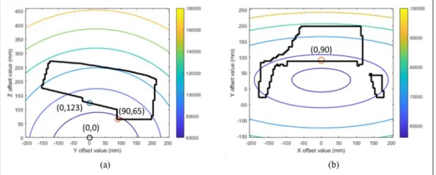
According to the workpiece’s machinable domain, it was found that the workpiece must be raised 123 mm along the Z-axis from the orginial workpiece setup posi-tion, so that the workpiece is machinable. Figure 10 shows a contour plot of the total axial movements dis-tance. The figure shows that the original setup position, the black ‘‘o’’ at (0, 0, 0), is not machinable. Within the constraint of the machinable domain, the modified setup position, the blue ‘‘o’’ at (0, 0, 123), gives the dis-tance of 64653 units. However, we can find an optimal setup position, the orange ‘‘o’’ at (0, 90, 65), to reduce
the distance. The global minimum of optimal setup position at (0, 90, 65) gives the shortest distance of 53,816 units.
Three parts with three different setup positions listed in Table 3 were machined, as illustrated in Figure 11. Because the part put at (0, 0, 0) is not machinable, we move the part to the modified setup position (0, 0, 123) to make it machinable, and the total axial movements was calculated as 64,653 units as listed in Table 3. The real machining time was 561 s. Then we set the part at the optimal setup position, and the total axial move-ments was calculated as 53,816 units, which was 16.76% less than the those for the part put at the
Figure 9. Toolpath for the channel: (a) left-side; (b) right-side.
Figure 10. Contour plot of axial movements results on the section (a) YZ plane at X0, and (b) XY plane at Z65. The boundaries of the cross section of the machinable domain are the black lines. The black ‘‘o’’ refers to the origin setup position, the blue ‘‘o’’ refers to the modified setup position and the orange ‘‘o’’ refers to the optimal setup position.
Table 3. Calculated and real machining results of the channel.
Workpiece setup position Distance Reduced distance Machining time Reduced time Machinable
Origin (X0, Y0, Z0) 42,169 2 2 2 No
Modified result (X0, Y0, Z123) 64,653 2 561 s 2 Yes
modified setup position. The machining time was 501 s, which was 10.70% less than that for the part put at the modified setup position. Because the total axial move-ments were very complicated, the reduction in distance was not very consistent with that in machining time. Based on the results, it is demonstrated that the algo-rithm proposed can find the optimum setup position to reduce the machining time effectively.
Conclusion
In this paper, we derived the kinematics for each type of five-axis machine tools. Then, we used the general transformation matrix to derive the optimization equation and the gradient descent method to find the global minimum. A case is presented to verify the proposed method and the total axial movements were reduced by 16.76%, and the machining time was reduced by 10.70% if we set up the workpiece at the optimal position. The proposed method can substan-tially reduce the machining time for the five-axis machining, which is practically important to the machining industry.
Acknowledgement
The authors wish to thank the Ministry of Science and Technology, Republic of China, for financial support of this research.
Declaration of conflicting interests
The author(s) declared no potential conflicts of interest with respect to the research, authorship, and/or publication of this article.
Funding
The author(s) disclosed receipt of the following financial sup-port for the research, authorship, and/or publication of this article: Ministry of Science and Technology, Republic of China, under Grant MOST 105-2221-E-011-055.
ORCID iDs
Ching-chih Wei https://orcid.org/0000-0002-7433-6645 Wei-chen Lee https://orcid.org/0000-0002-0672-0426
References
1. Denavit J. A kinematic notation for lower-pair mechan-isms based on matrices.Trans ASME J Appl Mech1955; 22: 215–221.
2. Lee RS and She CH. Developing a postprocessor for three types of five-axis machine tools.Int J Adv Manuf Technol1997; 13: 658-665.
3. Jung YH, Lee DW, Kim JS, et al. NC post-processor for 5-axis milling machine of table-rotating/tilting type. J Mater Process Technol2002; 130–131: 641–646.
4. She C-H and Lee R-S. A postprocessor based on the kinematics model for general five-axis machine tools. J Manuf Process2000; 2: 131–141.
5. She CH and Chang CC. Design of a generic five-axis postprocessor based on generalized kinematics model of machine tool. Int J Mach Tools Manuf 2007; 47: 537–545.
6. Sørby K. Inverse kinematics of five-axis machines near singular configurations. Int J Mach Tools Manuf 2007; 47: 299–306.
7. Yang J and Altintas Y. Generalized kinematics of five-axis serial machines with non-singular tool path genera-tion.Int J Mach Tools Manuf2013; 75: 119–132. 8. Lee R-S, Lin Y-H, Tseng M-Y, et al. Evaluation of
workpiece orientation and configuration of multi-axis machine tool using visibility cone analysis.Int J Comput Integr Manuf2010; 23: 630–639.
9. Hu P, Tang K and Lee C-H. Global obstacle avoidance and minimum workpiece setups in five-axis machining. Comput Aided Des2013; 45: 1222–1237.
10. Anotaipaiboon W, Makhanov SS and Bohez ELJ. Opti-mal setup for five-axis machining. Int J Mach Tools Manuf2006; 46: 964–977.
11. Tutunea-Fatan OR and Bhuiya MSH. Comparing the kinematic efficiency of five-axis machine tool configura-tions through nonlinearity errors. Comput-Aided Des 2011; 43: 1163–1172.
12. Lin Z, Fu J, Shen H, et al. On the workpiece setup opti-mization for five-axis machining with RTCP function.Int J Adv Manuf Technol2014; 74: 187–197.
13. Xu K and Tang K. Optimal workpiece setup for time-efficient and energy-saving five-axis machining of free-form surfaces.J Manuf Sci Eng2016; 139: 051003. 14. Shaw D and Ou G-Y. Reducing and axes movement of a
5-axis AC type milling machine by changing the location of the work-piece. Comput-Aided Des 2008; 40: 1033–1039.
15. Pessoles X, Landon Y, Segonds S, et al. Optimisation of workpiece setup for continuous five-axis milling: applica-tion to a five-axis BC type machining centre.Int J Adv Manuf Technol2012; 65: 67–79.
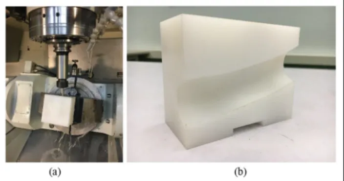
16. Xu H-Y, Hu La, Hon-yuen T, et al. A novel kinematic model for five-axis machine tools and its CNC applica-tions.Int J Adv Manuf Technol2013; 67: 1297–1307. Figure 11. (a) The real cutting process and (b) the section
17. Tulsyan S.Prediction and reduction of cycle time for five-axis CNC machine tools. Master Thesis, University of British Columbia, Canada, 2014.
18. Boyd S and Vandenberghe L.Convex optimization. Cam-bridge: Cambridge University Press, 2004.
19. Lee W-C and Wei C-C. Visualization of the setup loca-tion of a workpiece for five-axis machining.J Adv Mech
Des Syst Manuf 2019; 13: JAMDSM0042-JAMDSM0042.
20. Ravindran A, Ragsdell KM and Reklaitis GV. Engineer-ing optimization: methods and applications. 2nd ed. Berlin: Springer, 2007, pp.1–667.
Appendix
Notation
Variable Description Xi, Yi, Zi, Ai, CiThe machine coordinates of X, Y, Z, A, and C axis in segmentiof the toolpath. DXi,DYi,DZi,
DAi,DCi
The differences of machine coordinates X, Y, Z, A, and C axis between segmentiand segmenti-1of the toolpath
xi, yi, zi The workpiece coordinates of X, Y, and Z axis in segmentiof toolpath.
p, q, r The three elements of the offset vectordwalong the X, Y, and Z directions.
li, l The pseudo-distance of segmentiof the toolpath and the total pseudo-distance.
dorg,torg The toolpath distance and machining time in the original setup position.
dopt,topt The toolpath distance and machining time in the optimal setup position.
dR,tR The reduction of toolpath distance and machining time.
Vector Description
dM!S The vector from OMXYZ to OSXYZ. dS!T The vector from OSXYZ to OTXYZ. dM!4th The vector from OMXYZ to O4XYZ.
d4th!5th The vector from O4XYZ to O5XYZ.
d5th!W The vector from O5XYZ to OWXYZ.
dw The offset vector of workpiece movement from the original setup position. pi The machine coordinates of X, Y, and Z axis in segmentiof the toolpath.
Matrix Description
Ti The 4 4 homogeneous transformation matrix on the table side.
Si The 4 4 homogeneous transformation matrix on the tool side.
LTi,LSi The 3 1 matrices as the translation matrices inTiandSi.