Artificial Neural Networks for Gas Turbine Modeling and Sensor Validation

(1)

Artificial Neural Networks for

Gas Turbine Modeling and

Sensor Validation

Magnus Fast

Thesis for the Degree of Master of Science Division of Thermal Power Engineering Department of Energy Sciences

LUND UNIVERSITY

Faculty of Engineering LTH P.O. Box 118, S – 221 00 Lund Sweden

(2)

(3)

Artificial Neural Networks for

Gas Turbine Modeling and

Sensor Validation

Magnus Fast

December 2005 Master Thesis

Division of Thermal Power Engineering Department of Energy Sciences

Lund University, Sweden

(4)

ISRN LUTMDN/TMHP––06/5085––SE Printed in Sweden

(5)

Preface

This master thesis has been conducted at the division of Thermal Power Engineering, department of Energy Sciences, Lund University, Sweden. The work has come about in cooperation with Lunds Energi AB, during the fall of 2005.

This master thesis has been very educational in terms of implementing my knowledge in the field of gas turbine theory and combined heat- and power plants, as well as providing me with new knowledge about artificial neural networks and software accompanied with it.

I want to acknowledge my supervisors Mohsen Assadi and Jaime Arriagada for their support and profound knowledge in the fields described above. At Lunds Energi AB I would like to acknowledge Stefan Nilsson and Vinko Culjak for answering all my questions and providing me with necessary information to complete this master thesis.

I would also like to thank Mehrzad Kaiadi for our long discussions about artificial neural networks and the many conclusions we have drawn from them.

Finally I would like to thank my better half Alisa Selimovic for always supporting me no matter what I am doing.

Lund 2005-12-23

(6)

Abstract

The aim of this collaboration, between the division of Thermal Power Engineering and Lunds Energi AB, is to investigate the possibilities of training artificial neural networks (ANNs) with power plant operational data. For this purpose operational data from Lunds Energi’s gas turbine GT10B with heat recovery unit (HRU) will be used. Furthermore a model with user interface is created to demonstrate the possibilities of using ANN. The results are evaluated through feedback from Lunds Energi and many different areas of implementation are considered.

ANN differs from conventional mathematical models in the sense that they are trained rather than programmed. During training, data is presented in an iterative manner in order to find the relation between selected inputs and outputs. After the network is trained the weights, i.e. the parameters containing the network information, are locked and if the network is presented with new, before unseen, data it is able to predict new outputs.

The software used for modeling ANNs is called NeuroSolutions. The resulting networks have been processed in Visual Basic for final use in Excel.

Thru these studies several ANN models have been produced, both models of the gas turbine (GT) and models for sensor validation (SV). The results have been promising, e.g. with networks demonstrating high performance predictability.

(7)

List of Figures

Figure 2.1 Non-linear multi-dimensional system [2]. ... 5

Figure 2.2 Main ANN architectures [2]. ... 6

Figure 2.3 Schematic representation of an artificial neuron and common transfer functions [2]... 7

Figure 2.4 General structure of a single-layer feed-forward network. [2]. ... 8

Figure 2.5 Geometric representation of the discriminant function and the weights... 9

Figure 2.6 Gradient-based updating of the weights [2]. ... 12

Figure 2.7 Difference between linearly separable and non-linearly separable classes [2]. ... 13

Figure 2.8 Complex decision borders with hidden units [2]... 13

Figure 2.9 General structure of a two-layered feed-forward MLP [2]. ... 14

Figure 2.10 Pre-processing and post-processing of the data [2]. ... 16

Figure 2.11 Tuning the size of the hidden layer by trial and error [2]. ... 16

Figure 2.12 Overfitting of training data [2]. ... 17

Figure 4.1 Screen dump from Lunds Energi control panel [16]. ... 19

Figure 4.2 Screen dump from Lunds Energi control panel [16]. ... 20

Figure 4.3 Effect of flame temperature on NOx emissions [12]. ... 22

Figure 4.4 Dependence of emissions on fuel/air ratio [12]. ... 23

Figure 5.0 GT system modeled with two ANNs... 25

Figure 5.1 Higher calorific value variations for NG in February 2005 [6]... 28

Figure 5.2 Power output prediction for GT model. ... 29

Figure 5.3 Power output prediction for GT model without anti icing as input. ... 32

Figure 5.4 CO2 prediction for GT emission model... 34

Figure 5.5 User interface: GT model. ... 36

Figure 5.6 ANN for sensor validation [9]. ... 38

Figure 5.7 Confidence level plot with sensor Tcout,2 failing. ... 39

Figure 5.8 Confidence level plot with sensor Tcout,2 failing. ... 40

Figure 5.9 Confidence level plot with sensors Tcout,2 and T7 failing... 41

(10)

List of Tables

Table 2.0 Input and output signals... 4

Table 5.1 Parameters used for anti icing model. ... 26

Table 5.2 Predictive performance for anti icing model... 26

Table 5.3 Input parameters for GT model... 27

Table 5.4 Output parameters for GT model... 27

Table 5.5 Arbitrary input pattern and predicted outputs. ... 27

Table 5.6 Error distribution for the predictions from the GT model. ... 28

Table 5.7 Prediction errors for the GT model. ... 28

Table 5.8 Input parameter training intervals... 29

Table 5.9 Extrapolation: Original signals... 30

Table 5.10 Extrapolation: Predictions. ... 30

Table 5.11 Extrapolation: Errors. ... 30

Table 5.12 Prediction errors for the GT model without anti icing as input... 31

Table 5.13 Error distribution for the predictions from the GT model without anti icing as input... 31

Table 5.14 Prediction errors for the GT model with Tfuel as input... 32

Table 5.15 Prediction errors for the GT model without pamb as input... 33

Table 5.16 Prediction errors for the GT model without Tamb as input. ... 33

Table 5.17 Prediction errors for the GT model without RH as input. ... 33

Table 5.18 Output parameters for GT emission model. ... 34

Table 5.19 Prediction errors for the GT emission model. ... 34

Table 5.20 Comparison between recovered value and correct reading with a faulty sensor. ... 39

Table A.1 Network settings for anti icing model. ... 50

Table A.2 Network settings for GT model. ... 50

Table A.3 Network settings for GT model without anti icing... 50

Table A.4 Network settings for GT model with Tfuel... 50

Table A.5 Network settings for GT model without pamb... 51

Table A.6 Network setting for GT model without Tamb. ... 51

Table A.7 Network settings for GT model without RH. ... 51

Table A.8 Network setting for GT emissions model. ... 51

Table B.1 Network settings for GT SV model... 52

(11)

Nomenclature

d Desired output or target -

e Error -

E Error function - F Transfer function - H Number of hidden neurons -

m Mass flow rate kg/s M Number of input nodes -

n Iteration number - N Number of output nodes -

p Pressure bar

P Power W

Q Heat W

s Effective input to transfer function -

T Temperature °C

w Weight -

w Weight vector - x Input signal to neural network -

x Input vector -

y Output signal from neural network -

GREEK SYMBOLS α Alpha value - δ Delta term - η Efficiency % η Learning rate - Σ Summation function - SUBSCRIPTS amb Ambient dh District heating cout Compressor outlet e Electrical el Electrical

i Arbitrary node in the input layer j Arbitrary neuron in the hidden layer k Arbitrary neuron in the output layer 3 Compressor outlet

(12)

7 Turbine outlet 0 Bias

SUPERSCRIPTS

T Transposed (vector)

ABBREVIATIONS

ABB Asea Brown Boveri

ADALINE ADAptive LINear Element ANN Artificial Neural Network BP Back Propagation CL Confidence Level CV Cross-Validation GT Gas Turbine HRU Heat Recovery Unit LMS Least Mean Square

MLP Multi Layer Perceptron NG Natural Gas

NS NeuroSolutions RH Relative Humidity SV Sensor Validation TIT Turbine Inlet Temperature UHC Unburned HydroCarbons VB Visual Basic

(13)

1 Introduction

1.1 Background

The department of Energy Sciences at Lund University is the first in Sweden to evaluate ANNs potential within power plant applications.

This master thesis is based on previous work presented in a licentiate thesis and a doctoral thesis by PhD Jaime Arriagada [2,3]. Several models, e.g. fuel cell models, have been studied before and modeling a gas turbine with power plant operational data is a step in this development.

By creating a useful product, or a base for a product, for Lunds Energi AB, power companies might realize the potential of using ANN models and thereby make future investments in such projects.

ANN is used when modeling the gas turbine, which could be modeled with e.g. the heat- and mass balance program IPSEPro. The reason for using ANN instead of other programs is because once the software (NeuroSolutions) is mastered the models are produced very fast. The requirement is that operational data is available. The final product can be utilized by anyone, in contrary to IPSEPro models.

Lunds Energi are the providers of operational data, generated by their GT10B gas turbine and heat recovery unit. As they entered the project they had no knowledge about ANN, so the goal was ultimately to make them realize the potential. This was accomplished by producing a model of the gas turbine complete with user interface. This model is very easy to use and has in return opened their eyes for the possibilities of using ANN models in their daily work.

(14)

1.2 Objectives

• Understanding ANN and implementing that knowledge to create ANN models in NeuroSolutions.

• Investigate the possibilities of creating ANN models with operational data from the power plant.

• Recognize potential fields where Lunds Energi can benefit from using ANN models.

• Produce an interesting, useful and easy to use product.

• Presenting a base for future work

1.3 Limitations

When describing ANN multi-layer perceptrons (MLPs) are in focus and some networks, e.g. self-organizing, are completely left out of the discussion.

This master thesis will primarily focus on the gas turbine and models based on gas turbine operational data.

No effort has been done making the models universally functional, i.e. they might not be applicable on other gas turbine configurations.

1.4 Methodology

Literature studies and ANN simulations based on operational data is the foundation of this master thesis.

The simulation tool used is the commercial software program NeuroSolutions. Constant contact with my supervisors and personnel at Lunds Energi has guided me through the work.

(15)

1.5 Outline of the thesis

Chapter 2 explains ANN fundamentals. The first section is recommended to everyone, while sections 2.1 – 2.6 offer a more detailed description of ANN.

Chapter 3 briefly describes the software, NeuroSolutions, used for modeling the ANNs.

Chapter 4 gives a description of the gas turbine and heat recovery unit at Lunds Energi AB.

Chapter 5 contains the case study with results from the ANN models studied. Section 5.2 contains results from the GT models and section 5.3 results from the SV models.

(16)

2 Artificial Neural Networks

Artificial Neural Networks consist of a number of processing units, or artificial neurons, communicating with each other by sending signals thru weighted connections. In contrary to traditional mathematical models, which are programmed, ANNs learn the relations between selected inputs and outputs.

An ANN does not care what the actual relations between selected input and output parameters are but will instead find its own connections. The easiest way to look at an ANN is as a box that, when presented with input signals, generates output signals (see figure 2.1). An effort to explain what happens inside of this box is made in this chapter.

ANN is a sophisticated tool to use when the relations between input and output are complicated or even unknown.

For demonstrative purpose, a simple arbitrary equation (see equation 2.0) will act as the relation between input signals and output signals, where x represents the input and y the output. If input signals are presented to the equation an equal amount of output signals will be generated (see table 2.0).

3 x y

2

= (2.0)

TABLE 2.0 INPUT AND OUTPUT SIGNALS.

x (input) y (output) 3 3 6 12 9 27 12 48 15 75 18 108 21 147

In this case the equation is known and it is very easy to produce an output signal with a specific input signal. Lets imagine that the equation does not exist but the input and output signals do and it is still desirable to be able to produce output signals for new input signals. This is where ANN comes in handy with its ability to learn the relations between input and output signals, no matter how complicated they are. This is accomplished trough a process called learning, where the signals are presented to the ANN in an iterative manner. After the learning process is completed the network is locked and the information about the relationship between output and input is thereby stored. When a new input signal is presented to the network, lets say 10, the network will produce the output signal 33.33, or at least very close to (it depends on the success of the learning process). The accuracy of the ANN produced

(17)

outputs will be best in the interval 3-21, i.e. the interval used in the learning process. It is possible to train ANNs in a way that enables some extrapolation capability.

ANNs are not restricted to having only one input parameter and one output parameter but are also appropriate for modeling non-linear multi-dimensional systems, i.e. multiple inputs and outputs with non-linear relations (see figure 2.1).

The overall advantage, compared to traditional mathematical models, is that very complex systems can be modeled relatively fast, with the requirement that system data is available.

Non-linear system 1 2 3 . . . M Inputs 1 2 . . . N Outputs

FIGURE 2.1NON-LINEAR MULTI-DIMENSIONAL SYSTEM [2].

In this chapter, sections 2.1 – 2.4 provide the necessary background information for understanding section 2.5. This section describes the multi-layer feed-forward network, which is the network type used in chapter 5, case study, when modeling the gas turbine.

(18)

2.1 Network topology

ANNs are divided into two main groups depending on the topology of the connections, feed-forward and recurrent (feed-back) networks (see figure 2.2).

Feed-forward

Input Hidden Output

Feed-back (recurrent)

f(t) f(t-1)

f(t)

Input Hidden Output

Node Neuron

FIGURE 2.2 MAIN ANN ARCHITECTURES [2].

In this thesis, focus will be on feed-forward networks and as the name suggests signals are only allowed to pass in one direction, i.e. from input to output. Furthermore this ANN consists of different layers, one input layer, one or more hidden layers and one output layer. The communication between the environment and ANN consists of the input layer receiving data and the output layer delivering the computed results. The hidden layer communicates only within the network. If all units in one layer are connected to all units in the next layer it is called fully connected. No processing is done in the input layer and its components are called input nodes. Both the hidden layer and output layer are made up from artificial neurons, i.e. processing units.

The main objective for an artificial neuron is to receive weighted inputs from other neurons or nodes, compute an output and propagate this to other neurons. Another task is participating in the updating process of the connection weights during the learning process.

2.2 Basics of the learning process

Learning involves modifying the strength of connections between the elements. The learning process is called training and is performed according to learning rules, which are categorized in the two following groups:

• Supervised learning in which both inputs and desired outputs are known, this means the network can measure its predictive performance for given inputs.

• Unsupervised learning where only the inputs are known and the neurons must find a way to organize themselves without help from the outside.

After the training process is completed the weights are fixed. If new, previously unknown, inputs are presented to the network it will predict matching outputs. This ability is called generalization.

(19)

2.3 The artificial neuron

w_k0 w_kb y_k F Σ y_a y_b s_k neuron k

Linear function Threshold function

Log-sigmoid function tanh-sigmoid function y 0 0 s y y 0 y 0 +1 w_ka s s s

FIGURE 2.3 SCHEMATIC REPRESENTATION OF AN ARTIFICIAL NEURON AND COMMON TRANSFER FUNCTIONS

[2].

A specific neuron, k, joins the incoming signals, from other nodes or neurons, by a propagation function, normally standard summation. The resulting signal is called effective input, sk, and is passed thru a transfer function, F (different transfer

functions are described in section 2.3.1). The output signal from the neuron has the designation yk. The incoming signals have all been weighted, which means that they

are multiplied with respective weights (wka, wkb) equivalent to their significance for

neuron k. This means that the signals are either inhibited or exhibited. In addition to the input from nodes and neurons there is an extra input to every neuron, called the bias. The bias has the value +1 and the corresponding weight is wk0. The purpose is to

present an offset to the transfer function, which allows the neuron to have an output even if the input is equal to zero (see figure 2.5). The first letter in the indexes represents the destination neuron and the second letter represents the origin neuron. Equation 2.1 describes the process mathematically.

     = + =

∑

= ) s ( F y w ) w y ( s k k 0 k b a j kj j k (2.1)

2.3.1 Transfer functions

Different transfer functions are suited for different networks and applications, described below are four of the most commonly used:

The linear function (c = constant): s

c

(20)

The threshold function:    − ≥ + = otherwise , 1 0 s if , 1 y (2.3)

The logistic sigmoid function:

s e 1 1 y ₋ + = [0:1] (2.4)

The tanh sigmoid function:

s s s s e e e e y ₋ − + − = [−1:1] (2.5)

2.4 Single-layer feed-forward networks

x : inputs w: weights y : outputs Σ: Summation F : Transfer function x0=+1 xM w_N0 neuron k yk F Σ sk x1 . . . . . . . . . xi . . . y1 F Σ s1 yN F Σ sN node i w_k0 w₁₀ w_Niwki w_1i

FIGURE 2.4 GENERAL STRUCTURE OF A SINGLE-LAYER FEED-FORWARD NETWORK. [2].

The definition of single-layer network is that there is only one layer, i.e. output layer, with artificial neurons. They are used for classification tasks and for function approximation tasks [7]. Single-layer networks are accompanied by some disadvantages such as only being able of creating linear classifiers, demonstrated in figure 2.7 (page 13), or representing linear functions. One advantage towards multi-layer networks is that, because of their linearity, they always converge to one optimal solution.

2.4.1 Networks with threshold activation function

The simplest network has only one output neuron and two input nodes. The output from the network is either +1, if the effective input is positive, or -1 if the effective input is negative (see equation 2.3). The network can be used for classification tasks,

(21)

i.e. deciding whether an input pattern belongs to one of two classes. The output is given by following equation:

      ₊ =

∑

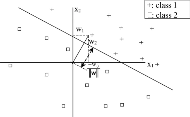
= 2 1 i 0 i ix w w F y (2.6)

The single layer network represents a linear discriminant function (equation 2.7) that acts as a decision border, separating the two classes.

2 0 1 2 1 2 0 2 2 1 1 w w x w w x 0 w x w x w − − = ⇔ = + + (2.7)

Figure 2.5 illustrates this function, and how the weights determine the slope of the line and the bias determines how far the line is from its origin, i.e. offset.

x2 x1 w2 w1 w 0 w − +: class 1 : class 2

FIGURE 2.5 GEOMETRIC REPRESENTATION OF THE DISCRIMINANT FUNCTION AND THE WEIGHTS.

The remaining issue is how to handle the learning of the weights. There are a variety of learning rules associated with the single-layer feed-forward network. Two of the most famous are the perceptron rule and the delta or least mean square (LMS) rule, which will be discussed in following sections. They both use supervised training (see section 2.2) and work iteratively to update their weights. This procedure can be described with these equations:

) n ( w ) n ( w ) 1 n ( w ) n ( w ) n ( w ) 1 n ( w 0 0 0 i i i ∆ + = + ∆ + = + (2.8)

The learning rules are actually different ways to compute ∆wi(n) and ∆w0(n), where n

(22)

2.4.2 The perceptron learning rule

Presuming we have a data set, with both inputs and desired outputs, an error can be defined with the difference between the desired output, also known as target, and the actual output: ) n ( y ) n ( d ) n ( e = − (2.9)

First of all the weighs are given random starting values and then an input vector is presented to the network, which will generate an error. The perceptron algorithm uses this error to calculate the next set of weights, i.e. the new weight vector (equation 2.10). After the weighs are updated a new input vector will be presented to the network and the procedure is repeated until something tells it to stop.

) n ( ) n ( e ) n ( ) 1 n ( w x w + = +η⋅ ⋅ (2.10) The learning rate factor, η, varies between 0 and +1. Contemplating the feed-forward threshold function network in section 2.4.1 the possible error outcomes are:

     − = + = = 2 e 2 e 0 e (2.11)

Corresponding equation for the bias:

0 0(n) e(n) x w ) 1 n ( + = +η⋅ ⋅ 0 w (2.12)

The following example demonstrates the iterative procedure of updating the weights. For every modification of the weights the discriminant function, illustrated in figure 2.5, is moved. Every modification makes the separation of the two classes more accurate. Two iterations are performed and the desired output can be either +1 or –1, representing the two classes.

(23)

2.4.2.1 Example of the perceptron learning rule

The network is initialized with following data:

5 . 0 , 2 ) 0 ( w , 2 1 ) 0 (  0 =− η=      = w Iteration #1 Input vector _      = 5 . 1 5 . 0 ) 0 (

x with the desired output d(0) = +1 is presented to the network.

The output is calculated according to equation 2.6, 1 ) 5 . 1 ( F ) 2 5 . 1 2 5 . 0 1 ( F ) 0 ( y = ⋅ + ⋅ − = =+

The error is calculated with equation 2.9 and since the output matches the desired output the error, e(0), adopts the value 0.

According to equation 2.10 the weight vector keeps its original values. Iteration #2 Input vector _      = 5 . 0 5 . 0 ) 1 (

x with the desired output d(1) = +1 is presented to the network.

The output is calculated according to equation 2.6, 1 ) 5 . 0 ( F ) 2 5 . 0 2 5 . 0 1 ( F ) 1 ( y = ⋅ + ⋅ − = − =−

The error is calculated with equation 2.9, e(1) = 2

The weights are altered according to equation 2.10 and 2.12:

1 1 2 5 . 0 2 ) 2 ( w 5 . 2 5 . 1 5 . 0 5 . 0 2 5 . 0 2 1 ) 2 ( 0 =− + ⋅ ⋅ =−       =       ⋅ ⋅ +       = w

2.4.3 The adaptive linear element

The adaptive linear element, ADALINE, was developed subsequent to the perceptron and uses the least mean square learning procedure, also known as the delta rule. The threshold transfer function has been replaced with a linear transfer function (see equation 2.2). An error function, E, is introduced and in order to find the optimal solution it has to be minimized.

(24)

) n ( e 2 1 ) ( E w = 2 (2.13)

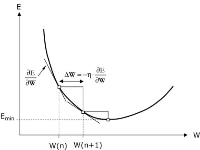
The error, defined in equation 2.9, can be expressed as: ) n ( ) n ( ) n ( d ) n ( e = −xT ⋅w (2.14) The main assumption is that the optimal weights are to be found in the direction of the descent gradient of the error function with respect to the weights (steepest descent method) [2], i.e.:

) n ( ) ( E ) n ( w w w ∂ ∂ η − = ∆ (2.15)

Differentiating equation 2.13 gives:

) n ( ) n ( e ) n ( e ) n ( ) ( E w w w ∂ ∂ = ∂ ∂ (2.16) Equation 2.14 and 2.16 gives:

) n ( ) n ( ) d ( ) n ( ) n ( e T _x w w x w ∂ =− ⋅ − ∂ = ∂ ∂ (2.17)

The final result, equation 2.18, becomes seemingly identical to equation 2.10 but in this case e is not limited to adopting the discrete values -2, 0 and +2.

) n ( ) n ( e ) n ( ) n ( ) n ( ) 1 n ( w w w x w + = +∆ = +η⋅ ⋅ (2.18) Figure 2.6 illustrates the gradient based learning method.

E W W(n) W(n+1) E_min W W ∂ ∂ ⋅ η − = ∆ E W ∂∂ E

(25)

2.5 Multi-layer feed-forward networks

2.5.1 Multi-layer perceptron

Multi-layer feed-forward networks are often called multi-layer perceptrons, because of their similarity to the perceptron [2]. The big advantages towards single-layer networks are that the MLPs are able to represent non-linear functions and classifying linearly separable classes. The difference between linearly separable and non-linearly separable classes is shown in figure 2.7.

o: class 1 o o o o o o

Linearly separable classes x1 x2 o o o o o o

Non-linearly separable classes x1

x2

misclassified : class 2

FIGURE 2.7 DIFFERENCE BETWEEN LINEARLY SEPARABLE AND NON-LINEARLY SEPARABLE CLASSES [2].

MLPs have at least one hidden layer but it has been proven that one layer with hidden neurons is enough to approximate any continuous function if it only has a sufficient number of units, provided the transfer functions of the hidden units are non-linear (see figure 2.8) [2]. Finding the sufficient number of hidden neurons, H, is a trial-and-error process.

Since the multi-layer perceptron has proven suitable for power plant applications other networks, such as self-organizing, will be left out of the discussion [2]. For more information on these networks Kröse’s An Introduction to Neural Networks [7] is recommended. o: class 1 o o o o o o

Non-linearly separable classes x1

x₂

3 hidden neurons Many hidden neurons : class 2

(26)

The general structure of a fully connected MLP, with M input nodes, H hidden neurons and N output neurons, is shown in figure 2.9.

w_kj wNj x : inputs w: weights y : outputs Σ : Summation F : Transfer function yH xo=+1 x_M wj0 neuron j w_H0 neuron k yj _y k F Σ sk F Σ sj F Σ sH x1 . . . . . . . . . . . . . . . +1 w1j xi . . . wji wiH y1 F Σ s1 yN F Σ sN node i

FIGURE 2.9 GENERAL STRUCTURE OF A TWO-LAYERED FEED-FORWARD MLP [2].

MLPs are trained in a supervised manner and they are most frequently trained with the back-propagation (BP) algorithm (described in section 2.5.2), originally known as the generalized delta rule. The advantages of MLPs have been known for a long time but it was not until in 1986, when Rumelhart, Hinton and Williams [11] presented the generalized delta rule, a satisfying way to update the weights was found. The original delta rule was only applicable on single-layer networks with linear transfer functions.

There are three different modes when training MLPs:

• Batch training: All available input patterns1

are presented to the network at the same time and an average error is calculated and then back propagated. The weights are updated and the process is repeated, i.e. the weights are updated epoch-by-epoch2

• Sequential training: Every input pattern is presented individually to the network and the weights are updated pattern-by-pattern.

• Block training: This is a combination of the techniques mentioned above. The input patterns are divided into blocks and the weights are updated block-by-block.

The batch-training mode is considered to be the most stable but it is also associated with slow convergence rate.

1

One input pattern is a group of inputs presented to the network at the same time and related to specific outputs.

2

One epoch is a cycle finished when all available training input patterns have been presented to the network once during training.

(27)

2.5.2 Back-Propagation

The back-propagation method is also called the generalized delta rule, which is a generalized form of the LMS rule. What makes this more complicated is that the error has to affect two sets of weights, i.e. the weights between hidden and output layer, and the weights between input and hidden layer. The back-propagation method requires differentiable transfer functions, e.g. sigmoid or hyperbolic, in order to modify the weights. The training can be divided into two phases:

• An error is calculated and the weights between the hidden and output layer are updated, comparable with the perceptron and the ADALINE.

• Since no information about the desired output from the hidden layer is available the error from the ouput layer is back propagated and used to update the weights between the input layer and the hidden layer.

BP is valid for networks with more than one hidden layer but, as stated before, one hidden layer with sufficient number of hidden units can approximate any continuous function. For a detailed description of the BP method, complete with equations, Arriagada’s Introduction of Intelligent Tools for Gas Turbine Based, Small-Scale Cogeneration [2] is recommended.

2.5.3 Data handling

An important aspect, not to be overlooked, in order to gain optimal results training MLPs, is the handling of available data. Following is to consider before, during and after training an ANN:

• Before starting any kind of training it must be realized that an ANN cannot become any better than the accuracy of the available data.

• A thorough review of the data to avoid and remove signals that are obviously distorted, i.e. outliers. If they are included in the training they might have a negative effect on the overall predictive performance of the network.

• The entire data set should be randomized and divided into a training set, a validation set and a test set. Different recommendations about the sizes of these sets are available but in general one third is used for testing while the rest is shared between the training and validation set. Approximately two thirds of this part is used for the training set and one third for the validation set. The training set is used to generate errors, which are used to update the weights, while the validation set is used to check the performance during training, to avoid over training (discussed in section 2.5.4). After the training is complete the test set is used to check the performance of the network with before unseen data, i.e. the nets generalization capability. This methodology is called cross-validation.

(28)

• Before introducing the data to the network it should be normalized to avoid that a signal with a value greater than the others does not become dominant. Normally data is linearly normalized within the boundaries for the transfer function output, e.g. [0,1] or [-1,1]. In order to understand the output signals, from the MLPs, they have to be de-normalized within the same boundaries. Figure 2.10 demonstrates this method.

ANN N o rm al iz at io n 1 0 500 50 D e-n or m a liz a ti on 350 0 1 0

input normalized input normalized output output

FIGURE 2.10 PRE-PROCESSING AND POST-PROCESSING OF THE DATA [2].

2.5.4 Overfitting

50 100 150 200 250 300 Epochs Training LMS-error Training goal very low H chosen H Increasing H Training #1 Training #2 Training #3 Final training . . .

FIGURE 2.11 TUNING THE SIZE OF THE HIDDEN LAYER BY TRIAL AND ERROR [2].

As mentioned before, finding the right number of hidden units is a trial-and error process, well illustrated in figure 2.11. This however can cause some problems with overfitting the network. This means that instead of having a good generalization capability, the network will simply memorize the training data. When choosing H, it is important to consider that the predictability for the training data will improve with increasing H but at some point the predictability for the validation and test data will worsen.

(29)

.

. ..

..

.

. . .

_{. .}

x y Overfitted, bad generalization

Good generalization Training data New inputs

FIGURE 2.12 OVERFITTING OF TRAINING DATA [2].

Overfitting can also occur if training is performed with too many epochs, i.e. learning iterations. Fortunately, this can easily be overcome by using the cross-validation method (described in section 2.5.3), which monitors the network during training and can perform an early stop if overfitting is detected. The overfitting is detected when the LMS error for the validation set starts to increase but the LMS error for the training set continues to decrease. Figure 2.12 shows an overfitted network.

2.6 Concluding remarks

The aim of this chapter is to provide knowledge about ANNs and specifically MLPs. Different networks, and the learning rules accompanied with them, are addressed. The basics of data handling before, during and after training are described. Furthermore overfitting, a long with measures avoiding it, is explained.

(30)

3 NeuroSolutions

All ANNs have been modeled with the commercial software program NeuroSolutions (NS).

There are six levels of NeuroSolutions, all of which allow you to implement your own neural models. The one used is the educator, the entry-level version, intended for those who want to learn about neural networks and work with MLPs. The users version extends the educator with a variety of neural models for static pattern recognition applications. The consultants version offers enhanced models that support dynamic pattern recognition, time-series prediction and process control problems. Furthermore, the consultant level offers the possibility to implement ANNs as DLL-files, which allows a smooth integration of finished ANNs into almost any software [10].

NeuroSolutions for Excel

NeuroSolutions for Excel is an Excel Add-in that integrates with any of the six levels of NeuroSolutions to provide a very powerful environment for manipulating your data, generating reports, and running batches of experiments [10].

3.1 Methodology

The gathering and pre-processing of data is performed in Excel with the assistance of additional, NeuroSolutions specific, commands. Input and output parameters are chosen, randomized and divided into sets (training, validation and testing).

The network is constructed in NS by means of selecting e.g. transfer functions, normalization boundaries and number of hidden units and epochs.

Once these steps are complete the training of the network can commence. NS offers the possibility of performing training variations, which simplifies the trial-and-error process of finding a satisfying number of hidden neurons (the best converging configuration will be saved). NS also offers the option of training with the cross-validation method and thereby avoiding overfitting of the network. A training report is created in Excel where the results for all the training variations can be studied.

Running all input patterns through the network and comparing the predicted outputs with the desired will test the predictive performance of the network.

The remaining issue is to create a user interface. This is accomplished by using the NS application, Formula Creator, which extracts the network to Visual Basic (VB) code, which in return can be employed as a function in Excel (after some adaptation of the VB code).

(31)

4 Lunds Energi: Gas Turbine and Heat Recovery

Unit

The GT and HRU with district heating system are illustrated schematically in figure 4.1 below. The GT produces electricity and large amounts of hot exhaust gases. The exhaust gases passes thru the HRU and heat is extracted to the district heating water, which is distributed to the consumers along with the produced electricity.

The positioning of the sensors, used to create the models in chapter 5, can also be seen in the figure.

(32)

4.1 The gas turbine

The gas turbine, GT10A, was installed by ABB STAL, now Siemens, in 1991 and rebuilt to a GT10B that same year. The GT10 is a lightweight industrial gas turbine (GT). The axial compressor has 10 stages and a pressure ratio of 13.6:1. The combustion chamber is annular and built for dual fuels, i.e. gas and liquid (at the moment Lunds Energi uses natural gas (NG)). The turbine has 2 stages where the first one is powering the compressor and the second one is connected to the generator. The turbine inlet temperature (TIT) can reach a maximum of 1062 °C and the GT has the capacity of producing 22 MW electricity [16]. The gas turbine is illustrated schematically in figure 4.2 below.

FIGURE 4.2 SCREEN DUMP FROM LUNDS ENERGI CONTROL PANEL [16].

4.1.1 Anti icing

If required anti icing air for the inlet is taken from the compressor delivery via a bleed-valve3

. The anti icing system prevents ice from forming in the intakes during

3

(33)

high humidity/cold ambient air conditions. The danger with ice reaching the compressor is the potential harm it can inflict on the airfoils.

The mass flow thru the gas turbine’s expander section will decrease and since the power output is directly dependant on this it will also decrease (see figure 5.2, page 29).

4.1.2 Performance degradation/deterioration

Even under normal engine operating conditions, with a good inlet filtration system, and using a clean fuel, the engine flow path components will become fouled, eroded, corroded, covered with rust scale, damaged, etc. The result will be deterioration in engine performance, which will get progressively worse with increased operating time. Three types of deterioration are recognized [5]:

• Performance deterioration recoverable with cleaning/washing.

• Performance deterioration non-recoverable with cleaning/washing.

• Permanent performance deterioration, which is not recoverable after an overhaul.

Recoverable deterioration is often caused by air-born particles, e.g. dirt, dust and pollen. The particles accumulate on the compressor airfoils and gas path surfaces (fouling the surfaces). Together with soot particles (NG is soot-free), produced in the combustor, they can also accumulate on the flow path surfaces in the turbine. Oil leaks and the presence of oily substances in the air can exacerbate the deterioration by acting as glue to the particles. Compressor fouling results in decreased mass flow and compressor efficiency. Hot-end fouling results in a reduction in the overall turbine efficiency. Three different methods of cleaning/washing the compressor are described below [5]:

• On-line4 dry cleaning of compressor with e.g. rice husks or pecan shells.

• On-line wash of compressor with water, water mixed with detergent, or some other suitable fluid, which is preferably nontoxic, nonflammable, and biodegradable.

• Off-line soak wash with suitable fluid

The last method described is the only one that requires a shut down of the gas turbine but is also the most efficient method, i.e. the one that gives a higher grade of recovery in GT performance.

4

(34)

4.1.3 Emissions

Gas turbine combustion is a steady flow process in which a hydrocarbon fuel is burned with a large amount of excess air, to keep the turbine inlet temperature at an appropriate value [12]. The exhaust gases are primarily a mixture of O2, N2, H2O and

CO2 but also include small proportions of e.g. NOx, CO and unburned

hydrocarbons (UHC). Although the proportions of the later mentioned emissions are very small, the large flow of exhaust gases produces a considerable amount of pollutants. The only way to minimize CO2 emissions, which is believed to contribute

to global warming, is to increase the efficiency of the gas turbine or by using non-fossil fuels.

4.1.3.1 NO_x, CO and UHC emissions

There are many different parameters affecting the amount of pollution created, e.g ambient conditions, load, flame temperature and residence time5. The most important factor, regarding the formation of NOx, is the flame temperature, which

has a maximum at stoichiometric conditions. The relationship between NOx

formation and flame temperature is seen in figure 4.3 below.

FIGURE 4.3 EFFECT OF FLAME TEMPERATURE ON NO_X EMISSIONS [12].

Operating far away from stoichiometric conditions (which gas turbines do) reduces NOx but unfortunately CO and UHC increases. The relationship can be seen in

figure 4.4.

5

(35)

FIGURE 4.4 DEPENDENCE OF EMISSIONS ON FUEL/AIR RATIO [12].

4.2 The heat recovery unit

The heat recovery unit produces hot water for the district heating system by extracting heat from the exhaust gases in an economizer and a gas condenser (see figure 4.1). By using the excess heat produced by the gas turbine the overall efficiency of the plant increases dramatically. Approximately 35 MW heat is extracted. A regulator that continuously adjusts the valves situated on the district heating pipes automatically controls the HRU. Thru this a constant gas temperature after the gas condenser, i.e. the temperature of the gas exiting the chimney, and a desirable district heating delivery temperature is maintained.

4.2.1 Degradation

Degradation of the HRU can occur, thru the formation of coatings on the heat exchanger surfaces, when burning e.g. coal or oil but when using natural gas this problem disappears. A more probable cause of degradation would be coatings forming on the inside of the heat exchangers because of substances present in the district heating water.

(36)

5 Case Study

In this chapter the possibilities of training ANN models, with actual operational data from the power plant (described in chapter 4), are examined. The available operational data consists of approximately 100 different parameters saved as minute averages, and they can be divided into the three following groups:

• Gas Turbine

• Heat Recovery Unit and District Heating

• Emissions

One of the first steps is to select the parameters that are of significance to the current model. This is primarily done with the author’s knowledge in the field of gas turbines and combined heat- and power plants. Different models will be studied and for each case unique combinations of parameters will be used.

Section 5.2 discusses GT models with performance predictions and section 5.3 considers the use of ANN sensor validation models. All ANNs are modeled in NeuroSolutions using MLP networks.

5.1 Data treatment

As mentioned in section 2.5.3 all data must be examined in order to discover distorted or unwanted data. For instance, this specific GT is always operated at full load but when the gas turbine is turned on there is a short period of time before the GT has reached its operating point. This data, corresponding to the start sequence, could be confusing for an ANN and simply worsen the predictive performance of the model. In a similar way, the data produced when the GT is turned off is meaningless for modeling purposes. Another thing to take into consideration is that a sensor can fail to deliver a correct value, e.g. the reading can be zero. If this remains undetected it can be devastating for the ANN model. Finally data with very large errors, i.e. outliers, has to be removed for the same purpose.

(37)

5.2 Gas turbine

Since there is a considerable amount of parameters available, two models will be trained separately (GT and emission models). This is done to simplify and hopefully improve the performance of the models.

Ambient conditions, i.e. relative humidity, atmospheric temperature and pressure, will be used as input and gas turbine parameters, e.g. power output, compressor discharge temperature and emissions, as outputs.

One initial problem encountered is that when the anti icing system is in operation the GT performance will differ significantly (for more information about anti icing, see section 4.1.1). Training an ANN with data both from when the anti icing system is in operation and when it is turned off can be compared with training an ANN with data from two different GTs. The obvious solution to this problem is to separate these data sets and train two different ANNs. A better and more sophisticated way to cope with the problem is to add an extra input parameter with the value 1 if the anti icing system is in operation and the value 0 otherwise. This will assist ANN to differentiate between the two cases (a comparison between an ANN with anti icing as input and one without is made in paragraph 5.2.2.2.1). The remaining issue is how to access this parameter. Since the ambient conditions control whether the anti icing system is in operation or not, it is possible to train an ANN with these conditions as input and anti icing as output. The system will then be modeled with both these ANNs (see figure 5.0). The output from the first (anti icing model) will act as input to the second (GT model). The results from the ANN anti icing model can be studied in this next section.

FIGURE 5.0 GT SYSTEM MODELED WITH TWO ANNS.

5.2.1 ANN anti icing model

Since data for the anti icing system does not exist it has to be produced manually, i.e. typed in by hand in Excel. This is accomplished by studying the compressor inlet temperature and when large leaps, within a small timeframe, are found it indicates that the anti icing system either is turned on or off. Table 5.1 demonstrates an arbitrary leap.

There is the possibility of recording the anti icing activity during GT operation, and thereby eliminating this procedure, but unfortunately there was no access to this kind of data during this master thesis.

(38)

TABLE 5.1 PARAMETERS USED FOR ANTI ICING MODEL. # Date/Time Relative humidity [%] Ambient pressure [mbar] Ambient temp. [°C] Comp. inlet temp. [°C] Anti icing [1-on:0-off] 695 2005-02-11 11:34 78.5 983.4 4.0 10.0 1 696 2005-02-11 11:35 78.2 983.3 4.0 9.8 1 697 2005-02-11 11:36 78.3 983.3 4.0 10.0 1 698 2005-02-11 11:37 78.4 983.5 4.0 10.0 1 699 2005-02-11 11:38 78.2 983.4 4.1 9.8 1 700 2005-02-11 11:39 78.0 983.4 4.1 10.1 1 701 2005-02-11 12:12 77.7 984.1 3.3 3.8 0 702 2005-02-11 12:13 77.8 984.2 3.3 3.8 0 703 2005-02-11 12:14 78.0 984.3 3.3 3.8 0 704 2005-02-11 12:15 78.1 984.1 3.3 3.7 0 695 2005-02-11 11:34 78.2 984.2 3.3 3.8 0

The transition is actually more gradual than the table shows but still very detectable (a closer look at the date/time column will reveal this). The reason for this is that data representing the transition period, i.e. the period from when the anti icing system is turned off until the GT has stabilized in its new operation point, has been removed because if included in training it can worsen the predictive performance of the ANN.

For the ANN anti icing model a data set with approximately 11.000 rows, which covers a week, will be used. During this period the anti icing system is turned on/off several times, enough for ANN to learn the relations between ambient conditions and anti icing. Relative humidity, ambient pressure and ambient temperature will be used as inputs. The compressor inlet temperature will not be used in training because it is not accessible before the GT is in operation. As mentioned before, anti icing will be used as the sole output. A training variation, 1-10 hidden neurons and a maximum of 5000 epochs, shows that the best results are attained with 8 hidden neurons and 5000 epochs (for more information about ANN specifics turn to chapter 2). The predictive performance for this ANN is shown in table 5.2.

TABLE 5.2 PREDICTIVE PERFORMANCE FOR ANTI ICING MODEL.

Correct Misclassified Quantity 10887 148 Share [%] 98.70 1.30

The results are considered acceptable and can be used as input in other ANNs. One possible origin of the missclassified data can be large gradients in the input parameters, e.g. ambient temperature, which could lead to a delayed start/stop of the anti icing system.

(39)

5.2.2 ANN GT model

Since the GT is operated at full load, it is assumed that only the ambient conditions and anti icing affects the performance. The input and output parameters used are:

TABLE 5.3 INPUT PARAMETERS FOR GT MODEL.

Input parameters Entity Anti icing 1 or 0 Relative Humidity % Ambient pressure mbar Ambient temperature °C

TABLE 5.4 OUTPUT PARAMETERS FOR GT MODEL.

Output parameters Entity

Airflow kg/s Compressor outlet pressure bar

Compressor outlet temperature °C Gas flow MJ/s Turbine outlet temperature °C Power output MW Generated heat MW

Although the generated heat is associated with the HRU it will be included because the whole system is in focus. The gas flow entity is [MJ/s] but still called a flow because it is merely multiplied with a constant calorific value [MJ/kg]. This model will not use the predicted values for anti icing but the manually produced (observe table 5.1), because it is desirable to separate potential errors origin. A training variation, with 1-10 hidden neurons and 10000 epochs, shows that the best network has 7 hidden neurons and is trained with 10000 epochs. Training with additional neurons, e.g. 11-20, will only improve the results marginally and is thereby considered unnecessary. Approximately 7500 rows of data are used for this training. An advantage of using large amount of data is that the contribution of eventual erroneous points will be very small and probably not affect the overall performance of the trained network. Table 5.5 demonstrates an arbitrary input pattern with its predicted outputs. Table 5.6 and 5.7 illustrates the error distribution, average and maximum error.

TABLE 5.5 ARBITRARY INPUT PATTERN AND PREDICTED OUTPUTS.

Input Signal Output Signal Predicted Error [%] Anti Icing 1 mair 66.03 66.26 0.36

RH 84.29 p_cout 12.68 12.71 0.26 p_amb 980.20 T_cout 365.87 365.86 0.00 Tamb 2.31 mNG 61.66 61.75 0.14 T₇ 513.41 513.36 0.01 P_el 19.06 19.16 0.54 Q_dh 34.25 34.33 0.25

(40)

TABLE 5.6 ERROR DISTRIBUTION FOR THE PREDICTIONS FROM THE GT MODEL.

Error [%] <1 1-2 2-4 >4

Airflow 7498 0 0 0

Compressor outlet pressure 7498 0 0 0 Compressor outlet temperature 7498 0 0 0 Gas flow 6950 548 0 0 Turbine outlet temperature 7498 0 0 0 Power output 7494 4 0 0 Generated heat 6328 1051 118 1

TABLE 5.7 PREDICTION ERRORS FOR THE GT MODEL.

Airflow Compressor outlet pressure Compressor outlet temperature Gas flow Turbine outlet temperature Power output Generated heat Average Error [%] 0.13 0.12 0.09 0.50 0.04 0.21 0.56 Maximum Error [%] 0.84 0.75 0.52 1.96 0.20 1.23 5.09

Good results are attained for most of the parameters and fairly good for the remaining. The gas flow and generated heat are the two parameters that have higher prediction errors. The generated heat is dependent on other parameters than the ambient conditions such as the district heat return temperature and flow. The reason for the slightly higher errors in gas flow predictions can be referred to the fact that no consideration to variations in the calorific value of the fuel (Danish natural gas) is taken. To increase the predictive performance for the gas flow, the calorific value should be added as an input to the network. Unfortunately this kind of data is not available for modeling so the results have to be accepted as they are. The variation in higher calorific value for the natural gas used in the GT is illustrated in figure 5.1. Another reason for the slightly higher error can be that gas flows are generally more difficult to measure with high accuracy.

(41)

17 18 19 20 21 22 23 2005-02-14 16:48:00 2005-02-14 19:12:00 2005-02-14 21:36:00 2005-02-15 00:00:00 2005-02-15 02:24:00 2005-02-15 04:48:00 2005-02-15 07:12:00 2005-02-15 09:36:00 2005-02-15 12:00:00 2005-02-15 14:24:00 2005-02-15 16:48:00 2005-02-15 19:12:00 Power [MW] 0 1 2 3 4 5 6 Error [%]

Pout [MW] Pout Predicted [MW] Error [%]

FIGURE 5.2 POWER OUTPUT PREDICTION FOR GT MODEL.

An arbitrary section of the data set including prediction values, for the power output, is presented in figure 5.2. The figure clearly shows when the anti icing system is in operation or not (high power output = anti icing off). It also shows ANNs capability of predicting the power output regardless of the anti icing systems influence.

The ramifications of using the predicted anti icing values, instead of the manually produced, would be that a certain amount (1.3%) of the input patterns would be misclassified (see table 5.2) and the predicted outputs would be totally wrong.

5.2.2.1 Extrapolation capabilities

The optimal network is achieved when training with data covering the whole operating range, while this specific network only uses data gathered during one week. The reason for not training with more extensive data is that data is usually not saved for a long period of time and waiting several months to get fresh data might not be an option (at least not during this master thesis). This leads us to the question of how the model will respond if presented with data outside of the training interval, i.e. the network’s extrapolation capability. For investigative purpose a random input parameter will be chosen, in this case ambient temperature. The interval, in which the temperature varies during training, is seen in table 5.8

TABLE 5.8 INPUT PARAMETER TRAINING INTERVALS.

RH p_amb T_amb

Max 91.99 996.66 4.06 Min 65.24 935.74 -4.50

(42)

An appropriate test data set with ambient temperatures outside of the training interval is used, in this data set the temperature varies from 4.5 °C to 13.5°C. The data is chosen so that the other input parameters remain within the same interval used when training the network. This means that the extrapolation capacity is tested with respect to the ambient temperature. Unfortunately the combustion chamber has been replaced in between the recording of these data sets and can cause the GT to behave differently. Anyhow, the following results are attained:

TABLE 5.9 EXTRAPOLATION: ORIGINAL SIGNALS.

INPUT OUTPUT Anti Icing RH p_amb T_amb m_air p_cout T_cout m_NG T₇ P_el Q_dh

0 79.8 986.2 4.5 69.4 13.4 363.8 65.9 506.1 20.7 35.6 0 76.4 986.0 5.5 69.2 13.3 363.8 65.6 506.6 20.6 35.6 0 77.9 984.6 6.5 68.6 13.2 363.8 65.1 507.7 20.3 35.2 0 71.8 982.4 7.5 68.0 13.1 363.8 64.4 508.7 20.0 35.6 0 74.2 980.2 8.5 67.3 13.0 365.6 63.8 509.4 19.8 34.8 0 88.9 976.0 9.5 66.5 12.8 365.5 62.6 510.9 19.4 34.7 0 72.2 976.0 10.5 66.0 12.6 365.6 63.1 512.2 19.1 33.5 0 89.5 973.7 11.5 65.4 12.6 365.5 61.4 512.7 19.0 34.6 0 90.0 973.6 12.5 64.9 12.6 367.3 61.1 513.7 18.8 33.7 0 90.3 973.7 13.5 64.6 12.5 367.3 60.7 514.0 18.7 34.1

TABLE 5.10 EXTRAPOLATION: PREDICTIONS.

INPUT PREDICTED Anti Icing RH p_amb T_amb m_air p_cout T_cout m_NG T₇ P_el Q_dh

0 79.8 986.2 4.5 68.7 13.1 361.6 64.2 507.4 20.2 35.4 0 76.4 986.0 5.5 68.1 13.0 361.4 63.3 508.2 19.9 35.2 0 77.9 984.6 6.5 67.3 12.9 361.3 62.3 509.1 19.6 34.9 0 71.8 982.4 7.5 66.8 12.8 360.9 61.7 509.7 19.4 34.7 0 74.2 980.2 8.5 66.2 12.7 360.7 61.0 510.4 19.2 34.5 0 88.9 976.0 9.5 65.2 12.5 362.4 60.2 511.2 18.8 34.1 0 72.2 976.0 10.5 65.4 12.5 360.4 60.3 511.3 18.9 34.1 0 89.5 973.7 11.5 64.7 12.4 362.4 59.7 511.9 18.6 33.8 0 90.0 973.6 12.5 64.5 12.4 362.5 59.6 512.2 18.6 33.7 0 90.3 973.7 13.5 64.3 12.3 362.6 59.5 512.3 18.5 33.6

TABLE 5.11 EXTRAPOLATION: ERRORS.

INPUT ERROR [%] Anti Icing RH p_amb T_amb m_air p_cout T_cout m_NG T₇ P_el Q_dh

0 79.8 986.2 4.5 1.1 1.7 0.6 2.7 0.3 2.3 0.6 0 76.4 986.0 5.5 1.6 2.2 0.7 3.6 0.3 3.1 1.2 0 77.9 984.6 6.5 1.9 2.4 0.7 4.2 0.3 3.4 0.8 0 71.8 982.4 7.5 1.7 2.3 0.8 4.1 0.2 2.9 2.5 0 74.2 980.2 8.5 1.7 2.4 1.3 4.3 0.2 3.3 0.9 0 88.9 976.0 9.5 2.0 2.5 0.8 3.8 0.1 3.2 1.5 0 72.2 976.0 10.5 0.9 0.9 1.4 4.5 0.2 1.1 1.7 0 89.5 973.7 11.5 1.2 1.8 0.8 2.8 0.1 1.9 2.2 0 90.0 973.6 12.5 0.7 1.6 1.3 2.5 0.3 1.3 0.2 0 90.3 973.7 13.5 0.5 1.4 1.3 2.1 0.3 0.8 1.4

As seen above, the predictions have larger errors but if this is caused by the new combustion chamber, bad extrapolation capability or both is hard to determine in

(43)

this study. One important conclusion drawn from the result is that the errors do not increase with increased ambient temperature. The trends of e.g. decreased power output and increased T7 are predicted well. All over the result is satisfying, giving a

hint of the actual values although training with a bigger interval, to avoid extrapolation, would be preferred.

5.2.2.2 Sensitivity analysis

The purpose of this paragraph is to understand the significance different inputs have on the network predictions. Both the influence of currently existing and supplementary inputs will be investigated.

5.2.2.2.1 ANN GT model without anti icing as input

Given the same prerequisites, as the original ANN GT model, an optimal network was found using 8 hidden neurons and 10000 epochs. The result is mediocre and it strengthens the statement that anti icing is a required input, made in section 5.2.

TABLE 5.12 PREDICTION ERRORS FOR THE GT MODEL WITHOUT ANTI ICING AS INPUT.

TABLE 5.13 ERROR DISTRIBUTION FOR THE PREDICTIONS FROM THE GT MODEL WITHOUT ANTI ICING AS INPUT.

Error [%] <1 1-2 2-4 >4

Airflow 6562 657 279 0

Compressor outlet pressure 6660 559 250 29 Compressor outlet temperature 7457 22 19 0 Gas flow 5747 1245 437 69 Turbine outlet temperature 7444 44 10 0 Power output 5858 987 495 158 Generated heat 5618 1518 338 24

(44)

17 18 19 20 21 22 23 2005-02-14 16:48:00 2005-02-14 19:12:00 2005-02-14 21:36:00 2005-02-15 00:00:00 2005-02-15 02:24:00 2005-02-15 04:48:00 2005-02-15 07:12:00 2005-02-15 09:36:00 2005-02-15 12:00:00 2005-02-15 14:24:00 2005-02-15 16:48:00 2005-02-15 19:12:00 Power [MW] 0 7 14 21 28 35 42 Error [%] Pout [MW] Pout predicted [MW] Error [%]

FIGURE 5.3 POWER OUTPUT PREDICTION FOR GT MODEL WITHOUT ANTI ICING AS INPUT.

For justification purpose the power output, with corresponding predictions, is plotted for the same time period as in figure 5.2. The predictive performance of the network has decreased dramatically after the anti icing input was removed. The maximum error for the power prediction is now over 12%.

5.2.2.2.2 ANN GT model with fuel temperature as input

The NG is preheated in order to maintain a specific temperature when it enters the combustion chamber. Nevertheless small variations occur and this changes the natural gas’s latent energy, which in return can create small variations in GT performance, e.g. changed gas flow. The purpose of this paragraph is to investigate the possibilities of enhancing the network’s predictive performance by including the NG temperature as an input. The best network, given the same prerequisites as the other models, was found using 10 hidden neurons and 10000 epochs. The mean and maximum errors are shown in table 5.14

TABLE 5.14 PREDICTION ERRORS FOR THE GT MODEL WITH T_FUEL AS INPUT.

The results show virtually no improvement in the predictive performance, so in conclusion the variations of the natural gas’s latent energy can be disregarded from and the first assumption, to only use ambient conditions (and anti icing) as inputs, is confirmed.

(45)

5.2.2.2.3 ANN GT model input variation

In this paragraph the three ambient conditions will be removed as inputs one at the time, to help understand their connection and importance to different output parameters. The same training variation as before is used and the errors can be studied in the tables below.

TABLE 5.15 PREDICTION ERRORS FOR THE GT MODEL WITHOUT P_AMB AS INPUT.

TABLE 5.16 PREDICTION ERRORS FOR THE GT MODEL WITHOUT T_AMB AS INPUT.

TABLE 5.17 PREDICTION ERRORS FOR THE GT MODEL WITHOUT RH AS INPUT.

In the first scenario, i.e. without ambient pressure as input, all output parameters are affected except compressor outlet temperature and turbine outlet temperature. In the second scenario all of the output parameters are affected more or less. The last scenario shows that the relative humidity has no effect on neither of the output parameters, which means that the ambient pressure and temperature (and anti icing which is not a parameter per se) are the only two parameters needed for modeling this GT (of course, the relative humidity is still needed for the anti icing model). This makes the result of the two first scenarios even more interesting, showing that with using only one parameter (relative humidity has no effect) it is possible to predict the outputs with fairly good accuracy, some even with the same precision.

5.2.3 ANN GT emission model

The same input parameters will be used for modeling the GT emissions but the probability of predicting all of them is low because they often depend on combustion chamber specific parameters (see paragraph 4.1.3.1) that are not accessible. For this task a section of data without the anti icing system turned on will be used (the influence of this parameter has already been demonstrated sufficiently).

(46)

The output parameters are:

TABLE 5.18 OUTPUT PARAMETERS FOR GT EMISSION MODEL.

Output parameters Entity

NOX ppm

CO %

CO₂ ppm

NO ppm

NO2 mg/MJ

TABLE 5.19 PREDICTION ERRORS FOR THE GT EMISSION MODEL.

NO_X CO CO₂ NO NO₂ Average Error [%] 3.48 3.60 0.43 6.04 1.96 Maximum Error [%] 22.25 26.51 4.75 37.07 14.05

The results in table 5.19 show that the presumption of difficult predictability is correct. The CO2 emissions are however predictable with reasonable small errors and

demonstrated in figure 5.4. Also seen in the figure is that the measured signal is not updated every minute, hence the constant values, and can contribute to the prediction errors.

Tests with alternative input parameters, e.g. turbine outlet temperature and gas flow, have been carried out but the results have all been alike. The probable cause is that these parameters are predictable with the ambient conditions and are thereby not contributing with new information to the network.

2.8 2.85 2.9 2.95 3 3.05 3.1 3.15 3.2 2005-10-23 04:48:00 2005-10-23 09:36:00 2005-10-23 14:24:00 2005-10-23 19:12:00 2005-10-24 00:00:00 2005-10-24 04:48:00 2005-10-24 09:36:00 2005-10-24 14:24:00 2005-10-24 19:12:00 2005-10-25 00:00:00 2005-10-25 04:48:00 Emission [%] 0 1 2 3 4 5 6 7 8 Error [%] CO2 CO2 predicted Error

(47)

5.2.4 Possible areas of implementation

In previous sections the performance for different ANNs are examined and evaluated. In this section, different possibilities regarding areas of application for the ANN models are discussed. As seen, some parameters are predicted with small errors and some are not, focus will be on the first category.

• Off-line modeling, i.e. when the GT is turned off. Considering that the ANN GT model only uses input parameters that are available at all time (i.e. ambient conditions), it is possible to predict e.g. power output, generated heat, gas flow and carbon dioxide emissions before start. This can prove helpful when evaluating if it is profitable or not starting the GT (with HRU). The power output and generated heat have direct economic dependencies since the power company is compensated per megawatt hour produced. The gas flow and CO2 emissions also have economic dependencies since the power

company disburses for consumed gas and produced CO2. All compensation

levels change continuously and deciding whether to start or not is rather complicated, so anything that facilitates this might prove useful. There is however lots of other considerations to take into account in the decision-making.

• On-line modeling, i.e. when the GT is in operation and automatically feeds the model with real-time data. Assuming the ANN model is trained with healthy GT data it is possible to compare the predicted values with the actual values and draw conclusions from that. For instance, if the power output decreases compared to the prediction it might intimate GT degradation and that the compressor needs washing (see 4.1.2). Comparably, decreased heat extraction could be a sign that the HRU is degraded (see 4.2.1). The model could also be used for fault diagnosis or an early warning system that indicates e.g. if a component is damaged. For more information about such a system Arriagada’s On the Analysis and Fault-Diagnosis Tools for Small-Scale Heat and Power Plants [3] is recommended.

Artificial Neural Networks for Gas Turbine Modeling and Sensor Validation

Artificial Neural Networks for

Gas Turbine Modeling and

Sensor Validation

Magnus Fast

Artificial Neural Networks for

Gas Turbine Modeling and

Sensor Validation

Magnus Fast

Preface

Abstract

Contents

List of Figures

List of Tables

Nomenclature

1 Introduction

1.1 Background

1.2 Objectives

1.3 Limitations

1.4 Methodology

1.5 Outline of the thesis

2 Artificial Neural Networks

2.1 Network topology

2.2 Basics of the learning process

2.3 The artificial neuron

∑

2.3.1 Transfer functions

2.4 Single-layer feed-forward networks

2.4.1 Networks with threshold activation function

∑

2.4.2 The perceptron learning rule

2.4.3 The adaptive linear element

2.5 Multi-layer feed-forward networks

2.5.1 Multi-layer perceptron

2.5.2 Back-Propagation

2.5.3 Data handling

2.5.4 Overfitting

.

. ..

..

.

.

. . .

. .

2.6 Concluding remarks

3 NeuroSolutions

3.1 Methodology

4 Lunds Energi: Gas Turbine and Heat Recovery

Unit

4.1 The gas turbine

4.1.1 Anti icing

4.1.2 Performance degradation/deterioration

4.1.3 Emissions

4.2 The heat recovery unit

4.2.1 Degradation

5 Case Study

5.1 Data treatment

5.2 Gas turbine

5.2.1 ANN anti icing model

5.2.2 ANN GT model

5.2.3 ANN GT emission model

5.2.4 Possible areas of implementation

_{. .}