Alma Mater Studiorum - Universit`a di Bologna
DOTTORATO DI RICERCA IN
Metodologia Statistica per la Ricerca Scientifica
XXVII Ciclo
Settore Concorsuale di afferenza: 13/D1 Settore Scientifico disciplinare: SECS-S/01
Differential expression analysis
for sequence count data
via mixtures of negative binomials
Presentata da Elisabetta Bonafede
Coordinatore Dottorato Relatori
Prof.ssa Angela Montanari Prof.ssa Cinzia Viroli Prof. St´ephane Robin
Abstract
The recent advent of Next-generation sequencing technologies has revolution-ized the way of analyzing the genome. This innovation allows to get deeper infor-mation at a lower cost and in less time, and provides data that are discrete mea-surements. One of the most important applications with these data is the differen-tial analysis, that is investigating if one gene exhibit a different expression level in correspondence of two (or more) biological conditions (such as disease states, treatments received and so on). As for the statistical analysis, the final aim will be statistical testing and for modeling these data the Negative Binomial distribution is considered the most adequate one especially because it allows for “over disper-sion”. However, the estimation of the dispersion parameter is a very delicate issue because few information are usually available for estimating it. Many strategies have been proposed, but they often result in procedures based on plug-in estimates, and in this thesis we show that this discrepancy between the estimation and the testing framework can lead to uncontrolled first-type errors. We propose a mix-ture model that allows each gene to share information with other genes that exhibit similar variability. Afterwards, three consistent statistical tests are developed for differential expression analysis. We show that the proposed method improves the sensitivity of detecting differentially expressed genes with respect to the common procedures, since it is the best one in reaching the nominal value for the first-type error, while keeping elevate power. The method is finally illustrated on prostate cancer RNA-seq data.
Acknowledgments
It is very hard to express my whole grateful in few lines: these three years have been very precious and enriching.
First of all, thanks to my supervisor Prof. Cinzia Viroli: thank you for all the patient and scrupulous support, and thanks for giving me not only significant sta-tistical teachings but also a very precious human example.
A great thanks is also for Prof. St´ephane Robin: thank you for all the interesting suggestions and for your helpfulness; working with you has been really stimulating, and the parisian months have been a very nice experience that I will never forget. Thanks to Prof. Angela Montanari, who has always been present in my academic life, and who has given to me the opportunity of helping her with teaching. Thanks to my thesis committee Prof. Marco Alf`o, Prof. Livio Finos and Prof. Luigi Ippoliti, who gave me interesting suggestions to improve this work.
Thanks also to Dr. Franck Picard, for his contribution at this work.
Thanks to my Ph.D. colleagues Linda, Giovanni, Sara, Elena and Arianna: it has been nice to share with you these intense years! Thanks also to the guys of the AgroParisTech, and especially to Eleanna, for all the moments that we have en-joyed together.
Finally, last but not least, a special thanks to my family, to Giacomo and to all my friends: if this experience has been so special, it is certainly also thanks to you.
Contents
1 Introduction 1
2 NGS technologies and differential analysis 5
2.1 NGS technologies and RNA-Seq data . . . 5
2.2 Differential Analysis . . . 6
2.3 State of the art . . . 7
2.3.1 edgeR . . . 8
2.3.2 DESeq . . . 10
2.3.3 DSS . . . 13
3 Mixtures of Negative Binomials 15 3.1 The Negative Binomial distribution . . . 15
3.1.1 Poisson-Gamma mixture model . . . 16
3.2 Finite mixture models . . . 17
3.3 Mixtures of Negative Binomials . . . 18
3.3.1 Estimation issues . . . 19
4 The proposed method 23 4.1 The proposal . . . 23
4.1.1 Modeling RNA-Seq data . . . 25
4.1.2 Estimation . . . 26
4.2 The proposed test statistics . . . 31
4.2.1 Variances for each test statistic . . . 32
5 A simulation study 35 5.1 Simulation A . . . 36
5.2 Simulation B . . . 39
ii CONTENTS
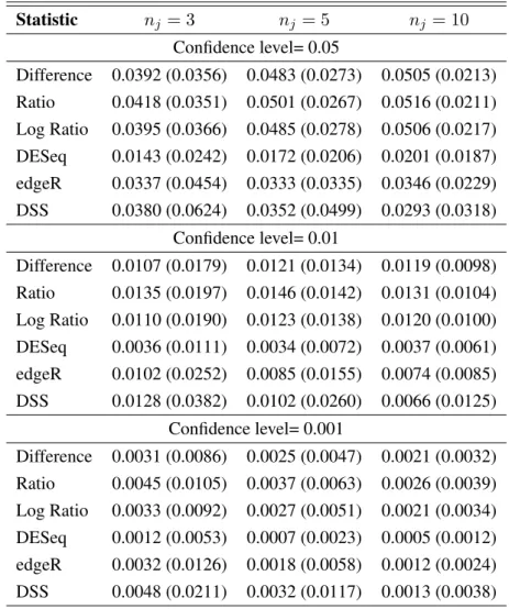
5.2.2 The first-type error . . . 42
5.2.3 The second-type error . . . 51
6 Application to Prostate Cancer Data 55 6.1 Normalization and explorative analyses . . . 56
6.2 Analysis and Results . . . 58
7 Concluding remarks 63 A Appendix 65 A.1 Appendix - Theλestimator . . . 65
A.2 Appendix - Simulation B . . . 66
A.2.1 First-type error . . . 66
A.2.2 Second-type error . . . 73
Chapter 1
Introduction
In the last decade the next-generation sequencing (NGS) assays, such as RNA-seq or ChIP-seq, have been revolutionizing the depth of understanding of the genome structure and the DNA or RNA interaction regions, due to the higher resolution of the data provided by these technologies [Soon et al., 2013, Wang et al., 2009]. From a statistical point of view, this innovation has gone along with a change in the nature of the data. Indeed, whilst the past mostly-used microarray technologies measured the abundance of a particular transcript as a fluorescence intensity expressed as continuous real data, the NGS experiments give read counts assigned to target genome regions, measuring the expression level or the abundance of the target transcript.
When the purpose of the assay is to performdifferential analysis, that is com-paring the counts of a given region between conditions, the statistical task is then to provide an appropriate model to account for biological and technical variations, as well as a testing framework to test the hypothesis of no difference. Here we deal with the case where regions of interest are givena priori, contrarily to analysis where the regions themselves have to be discovered [Frazee et al., 2014].
Generalized linear models based on count distributions now constitute a consensus framework for the analysis, with the original Poisson distribution [Marioni et al., 2008, Wang et al., 2010] being replaced by the Negative Bino-mial model [Robinson and Smyth, 2008, Anders and Huber, 2010, Robinson et al., 2010]. Indeed, the simplest choice of the Poisson distribution was rapidly identi-fied as the cause of uncontrolled first-type errors, due to a poor adjustment to the larger observed variability compared with the equal mean-variance specification of
2 1. Introduction
the Poisson model (see, for a discussion, Anders and Huber [2010]). Since then, the correct modeling and estimation of this observed overdispersion has been a key issue in differential analysis.
Taking perspective from our past experience in micro-array analysis, the proper modeling of the dispersion parameter has long been a subject of debate in differ-ential analysis, with a difficult trade-off between a common variance for every genes and gene-specific variances. Given the limited number of replicates, the first strategy provides robust estimates, but the testing procedure lacks of power and the model is not realistic, whereas the second is more sensitive at the price of increased first-type errors. Actually, the debate is still ongoing with the Negative Binomial framework, but the problem is much more difficult to solve due to this complex (and unknown) mean-variance relationship.
Several contributions have been proposed to find a trade-off between the com-mon overdispersion and the gene-specific overdispersion frameworks, and we will describe the three mostly used strategies in the next Chapter.
Despite the rapidly increasing diffusion of these statistical procedures, also thanks to the availability of several well documented Bioconductor packages, the estimation of the dispersion in NGS data remains a crucial and tricky issue because of the limited number of available observations for each gene. However, less atten-tion has been focused on the consistency between the estimaatten-tion and the testing frameworks. Indeed, many strategies consider the use of plug-in estimators, but an important drawback of this choice is that the expected variations of the test statistics are no longer controlled under the null hypothesis, which may result in an un-controlled level of the test. We will illustrate this point by a simulation study, showing that most proposed methods do not reach the nominal level of the test, whereas it is precisely what is expected to be controlled when performing standard hypothesis testing.
Our contribution is to explore and discuss a mixture model approach [McLachlan and Peel, 2000, Fraley and Raftery, 2002] based on the idea of shar-ing information among genes that exhibit similar dispersion. More specifically, mixtures of negative binomial distributions are investigated as a way to get more accurate estimations for the dispersion parameter of each gene, exploiting also the information provided by the others. Such an approach has already been considered in the same context for the differential analysis of microarray data [Delmar et al., 2005]. A consistent statistical testing procedure is then developed within the uni-fied model based clustering framework. The proposed method improves the
sen-3
sitivity of detecting differentially expressed genes with small replicates, and we show that our method controls the nominal level of the test by simulation.
A description of the procedures that provide these data together with a review of the most used methods that have been proposed in last years for performing differential analysis will be presented in Chapter 2. In Chapter 3 the negative binomial distribution and mixtures of negative binomials will be introduced. The novel method, together with the derivation of three statistical tests for performing the differential analysis will be described in Chapter 4. We will show through a large simulation study in Chapter 5 that the proposed statistical test procedure outperforms the mostly used strategies in the literature, because it is the best one in reaching the nominal value for the first-type error, while keeping elevate power, thus indicating its inferential reliability. The method will be applied on prostate cancer data in Chapter 6. A final discussion is presented in Chapter 7.
Chapter 2
NGS technologies and differential
analysis
2.1
NGS technologies and RNA-Seq data
The advent of the Next-Generation Sequencing (NGS) technologies has led to the production of sequencing platforms that allow to obtain high-throughput genomic data. These technologies can be used for many kinds of experiment, and in this work we will focus on those that lead to the analysis and the quantification of the transcriptome (that is the set of all RNA molecules), namely RNA-Seq data. The procedure for getting this kind of data can be summarized in three main steps [Oshlack et al., 2010]:
1. Sequencing: the studied transcriptome has to be preliminarily split into mil-lions of fragments. Thesequencingprocess produces theshort reads, that represent the sequence of the nucleotide basis that compose each fragment. Many types ofNGS sequencing platformshave been produced for this fun-damental procedure (among the others, 454 Genome Sequencer by Roche, Genome Analyzer by Illumina and SOLiD by Applied Biosystems). Each machine has its specific characteristics. We will not go into technical details, but as regards the mostly used one, the IlluminaGenome Analyzer, we can say that the samples are put on theflow-cellthat is a sequencing plate com-posed by several (usually 8)lanes(independent regions on the support). This makes possible to sequence different samples at once.
6 2. NGS technologies and differential analysis
location where a short read is identical (or, in practice, almost identical) to a reference genome or transcriptome.
3. Summarizing: after that as more reads as possible have been mapped on the genome, the data can be summarized simply by counting the number of readsoverlapping the exons (the codifying regions) in a gene.
As such, they are discrete measurements. It is important to underline that dif-ferent lanes could be characterized by difdif-ferentsequencing depth(orlibrary size), and potentially also by other technical effects. This makesnormalization proce-dures mandatory for comparative purpose (see, for instance, Bullard et al. [2010], Tarazona et al. [2011], Risso et al. [2011] and Dillies et al. [2013]), but in this the-sis we will not go into details of normalization methods.
The statistical procedures used for the analysis have to account for the features of count data, for the limited number of available information for each gene (due to high costs in sequencing procedures) and for the fact that NGS data are very often characterized by excess of zeros (inactivated regions).
2.2
Differential Analysis
Preliminaries: notation
RNA-seq data consist of nonnegative counts indicating the number of reads observed for each gene. Suppose we analyzepgenes inddifferent conditions, and on each of them observations are taken overnj replicates.
We denoteYijr the random variable that expresses the counts of reads mapped to
genei(i=1, ..., p), in conditionj(j=1, ..., d; in this work,d=2 w.l.g.), in sampler
(r=1, ..., nj).
Differential analysis
One of the most important and largely studied applications for NGS data is differential analysis, that is comparing the expression level of a specific gene (or exon) between samples observed in correspondence of two different biological con-ditions such as tissue types, disease states or treatments. Identifying differentially expressed genes could be a first step in detecting possible connections between one of these situations and the expression level of a specific gene [Kvam et al., 2012].
2.3 State of the art 7
From the statistical viewpoint, the differential analysis implies to perform sta-tistical testing to decide whether, for a given gene, an observed difference in read counts between two biological conditions is significant under a specific dis-crete probabilistic distribution or if it is just due to natural random variability [Anders and Huber, 2010]. The final aim consists in testing the null-hypothesis:
H0 :expression levelscondition 1 =expression levelscondition 2.
The benchmark distribution for count data is the Poisson [Cameron and Trivedi, 1998], but it can be too restrictive because it implies that variance and mean are equal (“equi-dispersion” property), while the RNA-seq data could be characterized by higher dispersion, leading to the so-called “over-dispersion problem”, and therefore the resulting statistical test would be unreliable.
The quasi-Poisson model had been proposed as alternative [Ismail and Zamani, 2013], which is fitted on the basis of a quasi-likelihood function, specifying a rela-tionship between the mean and the variance. However the provided estimators do not have great properties.
A more appropriate distribution is the negative binomial (NB), that is characterized by two parameters (a mean and a dispersion one) where the variance is a function of both oh them. For a deeper description of the NB distribution we refer to Section 3.1. A severe issue associated with this probabilistic framework is the reliable esti-mation of thedispersionparameter, reinforced by the limited number of replicates generally observable for each gene.
2.3
State of the art
Differential expression analysis is a largely studied application of RNA-Seq data, and many works have been published about it; here we report a brief overview of the mostly known ones. Bloom et al. [2009] have proposed to use the Fisher’s exact test for comparing the proportion of reads mapped to each gene in correspon-dence of different conditions.
Several strategies arose considering the Poisson distribution as reference for mod-eling the data. Among the others, Marioni et al. [2008] have fitted a Poisson model, thus performing aχ2 goodness of fit test; Bullard et al. [2010] have explored the likelihood ratio test possibility. Wang et al. [2010] have assumed the normality
8 2. NGS technologies and differential analysis
distribution for the log ratios of the counts and thus have computed a z-score, pro-viding anR package that is calledDEGseq (available on Bioconductor); Li et al. [2011] proposed a score statistic on the basis of a Poisson log-linear model, pro-viding an R package that is called PoissonSeq (available on CRAN). Various ap-proaches based on the negative binomial distribution have been studied, for han-dling the overdispersion problem. Hardcastle and Kelly [2010] proposed to itera-tively estimate the dispersion using the quasi-likelihood approach, thus providing a ranking of the genes on the basis of the posterior probabilities of being DE instead of the classical p-values; they published theRpackagebaySeq. Zhou and Wright [2011], with theirRpackageBBSeq, modeled the dispersions on the means, thus computing a Wald test. Other three strategies, probably the mostly used at all, are described in next sections with much more detail. These strategies have lead to largely usedRpackages, available and well documented from Bioconductor: DE-Seq,edgeRandDSS. We will present each method assuming that we are comparing justd= 2different biological conditions.
2.3.1 edgeR
Robinson and Smyth (Robinson and Smyth [2007], Robinson and Smyth [2008]) proposed to estimate a common dispersion parameter for all genes ex-pressed as a quadratic combination of the mean, and then, by making use of a weighted likelihood procedure, they provide an estimation of each dispersion pa-rameter as a weighted combination of the common and of the individual ones, as-suming empirical weights. Then an approximation is introduced in order to develop an exact test. This procedure is available in theRpackageedgeR[Robinson et al., 2010].
The model
Let us assume a NB distribution for the random variable Yijr that describes
the counts for geneiin the r −th sample of condition j: Yijr ∼ N B(µijr, ϕ)
whereϕis the dispersion parameter such thatE(Yijr) = µijr andV ar(Yijr) =
µijr(1 +µijrϕ). Let us suppose that E(Yijr) = µijr = sjrλij such that λij
describes the real abundance of transcripts for gene i in condition j and sjr is
thesize factor. Performing differential expression analysis means to test the null hypothesis
2.3 State of the art 9
Robinson and Smyth [2008] have proposed a new way for estimating the disper-sion parameter with this kind of data, that consists in making use of the information provided from all genes in order to estimate a common dispersionϕ, maximizing the common likelihood functionlC(ϕ).
Afterwards, they applied a quantile adjustment for avoiding problems due to differences in sample sizes.
The assumption of common dispersion is a good way for gain more stable results but it is not realistic for this kind of data, and therefore an Empirical Bayesian strategy has been proposed. Such procedure had already been applied to microarray data [Smyth, 2004]. The idea is to use a weighted conditional log-likelihood for estimating each gene-wise dispersionϕi(WL(ϕi)):
W L(ϕi) =li(ϕi) +αlC(ϕi) (2.1)
where we can recognize a special case of weighted likelihood [Wang, 2006], where the common likelihood rules as a prior for ϕi and α plays the rule of the prior
precision. The value for α has to be chosen accordingly to the strength of the similarity between the different dispersion parameters: the greater isα, the stronger is the effect of the common component.
As regards the selection of an appropriate value for α, first of all they have introduced their strategy considering a hierarchical model assuming (ideally) that the gene-specific estimatorsϕbiwere normally distributed: ϕbi|ϕi ∼N(ϕi, τi2)and
ϕi∼N(ϕ0, τ02). The Bayes posterior mean estimator ofϕi would be:
b ϕBi =E(ϕi|ϕbi) = b ϕi/τi2+ϕ0/τ02 1/τ2 i + 1/τ02 . (2.2)
ϕ0 andτ0 can be estimated from the marginal distribution ofϕbi to get a EB
rule. Under this idealistic model, we could derive:
b ϕW Li = b ϕi/τi2+α ∑d j=1ϕj/τj2 1/τ2 i +α ∑d j=11/τj2 , (2.3)
that coincides with the (2.2) for ϕ0 = ϕb0 =
∑p i=1ϕbi/τi2 ∑p i=11/τi2 and 1/α = ∑p
i=1τ02/τi2. As for the estimation ofτ02, under the normal model we would have that(ϕbi −ϕ0)2/(τi2 +τ02) ∼ χ21, so that a consistent estimator forτ02 could be
10 2. NGS technologies and differential analysis computed by solving: p ∑ i=1 ( (ϕbi−ϕb0)2 τ2 i +τ02 −1 ) = 0. (2.4)
In practice the individual estimatorsϕbi are not normally distributed and we do
not know their variances, but since the score statistics converge to normality more rapidly than maximum likelihood (ML) estimators and (2.4) can be written in terms of the score likelihood function and the expected information, they have proposed the following algorithm: first of all they have estimated the common dispersionϕb0, maximizinglC; then they evaluated, for each gene, the score functionSi(ϕb0) =
∂li(ϕb0)/∂(ϕb0) and the expected information Ii(ϕb0) = E(−∂2li(ϕb0)/∂ϕb20). Af-terwards they estimatedτ0 by solving
∑p i=1 ( S2 i Ii(1+Iiτ02)− 1 )
= 0 and they set 1/α=τ02∑ip=1Ii and finally they got weighted likelihood estimatorsϕei by
maxi-mizingW L(ϕi).
This way, ifϕi =ϕ0fori= 1, . . . , pthenE(S2i) =Iiso thatτ0will be estimated close to 0 andαwill be large. Conversely, if the gene-specific dispersion parame-ters are dissimilar, the algorithm will account for that proposing greater values for
τ0(and therefore weakening the shrinkage effect).
Testing for differential expression
After computing the dispersion parameters through the Empirical Bayes esti-mator, Robinson and Smyth [2007] have proposed an exact test analogous to the Fisher’s one. It is adapted for this kind of data, replacing the hypergeometric prob-abilities with negative binomial ones and conditioning on the sum of all the reads that are mapped to genei. For doing so, they had needed to introduce an approx-imation considering the normalized data as identically distributed. Finally they computed the exact p-values as the probabilities of observing counts as or more extreme than the observed.
2.3.2 DESeq
Anders and Huber [2010] proposed to use a mean-dependent local regression to smooth the gene-specific dispersion estimates, related to the idea that genes that share a similar mean expression level have also a similar variance, and therefore they can contribute to the estimation of the respective parameters. The method is
2.3 State of the art 11
implemented in theDESeqRpackage, available from Bioconductor. The model
We denote Yijr the number of reads that have been mapped to geneiin
con-ditionj, for sampler. DESeq assumesYijr ∼ N B(µijr, σijr2 ) whereµijr is the
mean andσijr2 is the variance. The meanµij is supposed to be equal toλijsjr, that
is the product of two terms: the first one is proportional to the real abundance of transcripts for geneiin conditionj, and the latter is the size factor, that is lane-dependent. The varianceσ2ijris the sum of two components:σijr2 =µijr+s2jrνij.
The first one is calledshot noise, and it is the variance that would be computed as-suming a Poisson model for the data. The second is theraw variance termand it is supposed to be a smooth function ofλij. The novel aspect of this strategy consists
indeed in considering that the estimation of theoverdispersioncomponent can be gained pooling information among genes that exhibit a similar expression level. This model requires the estimation of three sets of parameters:
• the size factorssjr(for each samplerin conditionj),
• the expression strength parametersλij (for each geneiin conditionj),
• the smooth functionsνj : ℜ+ → ℜ+ (for each conditionj), for modeling
the dependence of the raw variancesνij on the expectationsλij .
As regards the first set of parameters, Anders and Huber [2010] have proposed a new way for computing the library sizessjr, that is:
b
sjr =mediani
yijr
(∏j∏ryijr)1/n
,
wherenis the total number of samples (n=∑2j=1nj), and the denominator is a
geometric mean of the counts computed on theninformation available for genei. For the estimation of the expression level,
b λij = 1 nj nj ∑ r=1 yijr b sjr . (2.5)
12 2. NGS technologies and differential analysis
As regards the νj, first of all they have computed the sample variances for the
normalized counts: ωij = 1 nj −1 nj ∑ r=1 ( yijr b sjr − b λijr )2 , (2.6)
and they have defined:
zij = b λij nj nj ∑ r=1 1 b sjr . (2.7)
It can be proved thatνij =ωij−zij is an unbiased estimator for the raw variance.
Nevertheless, the limitedness of the number of observations that are usually col-lected make theωij very variable, leading to unreliable estimates. Therefore the
authors have suggested to fit a local regression model on (bλij, ωij) to get a smooth
functionνj(λ)withνbj(λbij) =ωj(bλij)−zij as estimation of the raw variance.
Testing for differential expression
The differential expression analysis consists in testing the null hypothesis
λi1 =λi2, fori= 1, . . . , p. Anders and Huber [2010] have derived a test statistic that is the total counts in each condition:Yi1 =
∑n1
r=1Yi1randYi2 =
∑n2
r=1Yi2r; we define also the overall sumYi+=Yi1+Yi2. For each pair of values(a, b), with
a+b = yi+, they needed to compute the probability of the events: Yi1 =aand
Yi2 =band we denote it asp(a, b). The p-value of a pair of observed count sums (yi1, yi2) has been defined as:
pi= ∑ a+b=yi+ p(a,b)≤p(yi1,yi2) p(a, b) ∑ a+b=yi+p(a, b) . (2.8)
They assume that, under the null hypothesis, the samples are independents:
p(a, b) =p(Yi1=a)p(Yi2 =b).
Yi1 andYi2 are sums of NB random variables, and they suggested to approximate their distribution by a NB. For the derivation of the parameters, first of all they computedbλi0 = ∑d j=1 ∑nj r=1 yijr
sjr (pooling the counts of all conditions), that is
an average on all the normalized information for genei, considering the hypoth-esisλi1 = λi2 as true. The final mean and variance parameters of the resulting NB distribution are: µbij = ∑nj r=1sjrbλi0andσb2ij = ∑nj r=1bsjrbλi0+bs2jrbνj(bλi0)for j= 1,2.
2.3 State of the art 13
2.3.3 DSS
Wu et al. [2013] introduced an empirical Bayes shrinkage approach choosing a log-normal prior distribution on the dispersion parameters and therefore impos-ing a negative binomial likelihood. Then the estimations are plugged-in the Wald statistic to perform the statistical test. The method is implemented in theDSS R library.
The model
Wu et al. [2013] have assumed a hierarchical model:
ϕi ∼log−N ormal(m0, τ2) y θij|ϕi∼Gamma(λij, ϕi) y Yijr|θij ∼P oisson(θijsjr)
The marginal distribution ofYijr givenλij andϕi is a NB with meanµijr =
λijsjr(whereλij describes the real abundance of transcripts for geneiin condition
j,sjr is the library size), and dispersionϕi, that is variance equal toλij +ϕiλ2ij.
As it is well known there is not a conjugate prior forϕi, and they imposed a prior
that seems to reflect the empirical behavior of the dispersion parameters, that is the log-normal distribution.
It is possible to derive a conditional posterior distribution ofϕigiven all observed
counts and means:
log(p(ϕi|Yijr, µijr, j = 1,2;r= 1, . . . , nj)
) ∝ ∑ j,r ψ(ϕ−i 1+Yijr)−nψ(ϕ−i 1)−ϕ− 1 i ∑ j,r log(1 +µijrϕi) +∑ i Yijr (
log(µijrϕi)−log(1 +µijrϕi)
) −(log(ϕi)−m0)2
2τ2 −log(ϕi)−log(τ) (2.9) wheren=∑jnjis the number of samples. We could consider the posterior mean
14 2. NGS technologies and differential analysis
they propose to compute the posterior mode by maximizing an approximation of (2.9). In practice, they substituteµijr by µbijr = λbijsjrwhereλbij =
∑
rYijr/sjr
nj ,
and they plug-in the two hyper-parametersm0 and τ2 by pooling the data pro-vided by all genes. Finally they maximized the approximated equation (2.9) using the Newton-Raphson method. The estimatedϕbis an empirical Bayes estimator, shrunken toward the common prior.
Testing for differential expression
Performing differential analysis means testing the null hypothesisλi1 = λi2, fori= 1, . . . , p.
For this aim, they simply proposed to use the estimated parameters to plug-in the Wald test: ti = b λi1−bλi2 b σ2 i1+bσi22 (2.10) where σb2ij is the estimated variance for λij: σb2ij = 1/n2j(bλij(
∑nj
r=11/sjr) +
njbλ2ijϕi
)
Chapter 3
Mixtures of Negative Binomials
As it has already been explained, the Negative Binomial (NB) distribution is an appropriate choice for fitting RNA-Seq data. The analysis of these data requires to work with few replicates for each gene in each condition. Statistical strategies involving mixture models could provide additional flexibility and could be useful for sharing information among genes that exhibit similar features, thus leading to more reliable estimations.
In this chapter we are going to describe the NB and mixtures of NB distributions, and in the next chapter we will illustrate the usefulness of this strategy in perform-ing differential analysis.
3.1
The Negative Binomial distribution
As reported in Hilbe 2011 (Hilbe [2011]), theNegative Binomial probability density function can be defined according to several parameterizations. Among these, the so-called Negative Binomial 2 (NB2) is convenient because it is charac-terized by two parameters that are particularly related to its moments: the first one corresponds to the expectation and the second one has a particular role to deter-mine the variance.
Let us define a random variabley∼N egBin(λ, α)withλ,α >0and
E(y) =λ, V ar(y) =λ ( 1 + 1 αλ ) ;
16 3. Mixtures of Negative Binomials Y has density: f(y|λ, α) = ( y+α−1 α−1 ) ( λ λ+α )y( α λ+α )α . (3.1)
It is possible to show that (3.1) reduces to the Poisson forα→ ∞.
An interesting characteristic of this parametrization is that it can be derived from a Poisson-Gamma mixture model, by considering a random variable having a Poisson distribution with parameter depending on a second random variable distributed according to a Gamma distribution with mean equal to 1.
3.1.1 Poisson-Gamma mixture model
Let us define:
• a random variable u following aGamma(α, β)distribution (withα,β >0) such that f(u;α, β) = β α Γ(α)u α−1e−βu withE(u) = αβ andV ar(u) = βα2 .
We haveE(u) = 1forα=β and
f(u;α, α) = α
α
Γ(α)u
α−1e−αu
• a random variable y that conditional on u follows aP oisson(λu)distribution (withλ >0) such that
f(y;λu) = e
−λu(λu)y
y! withE(y) =V ar(y) =λu.
Then if we consider the following structure:
u∼Gamma(α, α)
y
3.2 Finite mixture models 17
it can be proved that Y is marginally distributed according to:
y∼N egBin(λ, α).
This means that the parameterλof the Poisson component rules the expectation of the negative binomial distribution, and the parameterαof the Gamma component controls the heterogeneity, allowing overdispersion.
3.2
Finite mixture models
The history of finite mixture models goes back to the end of the XIX century, when the famous biometrician Karl Pearson (Pearson [1894]) fitted a mixture of two normal probability density functions with different means and variances to some data about measurements on the ratio of forehead to body length of 1000 crabs sampled from the Bay of Naples, suggesting that there were two subspecies present.
“When a series of measurements gives rise to a normal curve, we may probably assume something approaching a stable condition; there is production and destruction impartially round the mean. In the case of certain biological, sociological, and economic measurements there is, however, a well-marked deviation from this normal shape, and it becomes important to determine the direction and amount of such de-viation. The asymmetry may arise from the fact that the units grouped together in the measured material are not really homogeneous. It may happen that we have a mixture of 2, 3, ... n homogeneous groups, each of which deviates about its own mean symmetrically and in a man-ner represented with sufficient accuracy by the normal curve. Thus an abnormal frequency-curve may be really built up of normal curves having parallel but not necessarily coincident axes and different pa-rameters.”(Pearson [1894])
We denote y = {y1, ..., yi, ..., yp} a random sample of sizep whereyi is a
n-dimensional random vector (withn=∑jnj) with probability density function
f(yi). If we suppose a K-component mixture model we can write it in parametric form as: f(yi;θ) = K ∑ k=1 wkfk(yi;θ), (3.2)
18 3. Mixtures of Negative Binomials
where the vectorθcontains all the unknown parameters in the mixture model, i.e. the parameters of the K probability density functionsfkof the K components and
the K weightswk, i.e. the mixing proportions (with the constraints0 ≤ wk ≤ 1
and∑Kk=1wk= 1).
The data matrix y is called “incomplete” since we actually do not know at which one of the mixture components each unit belongs. A new random variable
z = {z1, ..., zi, ..., zp}is then introduced, called “allocation variable”; zi will be
aK−dimensional vector of zeros except from the element that is in the position corresponding to the mixture-component at which thei−thunit belongs.
We will denotezik = 1when
zi= [ 0 0 . . . 1 . . . 0 ] ↑ kthposition
Thuszi is assumed to be distributed according to a Multinomial distribution,
and in particular:
zi ∼M ultin(1;w1, ..., wK) (3.3)
We consider now y and z all together we have the “complete data”, where y has been observed whilst z is hidden. If the label z of each observation was known, it would be easy to estimate the mixture parameters. However z is a hidden variable, hence it is very difficult to reach closed form formulas for the parameters and it is often complicated to estimate them. We will see in the next section one of the available algorithms to do it.
3.3
Mixtures of Negative Binomials
We consider a random variableyithat follows a K-component mixture model of NB distributions: f(yi;θ) = K ∑ k=1 wkfk(yi;θk) = K ∑ k=1 wkN Bk(λk, αk), (3.4)
3.3 Mixtures of Negative Binomials 19 that is: f(yi;θ) = K ∑ k=1 wk ( yi+αk−1 αk−1 ) ( λk λk+αk )yi( α k λk+αk )αk (3.5)
and therefore yi|zi ∼ N egBin(λk, αk) hence E(yi|zi) = λk and
V ar(yi|zi) =λk ( 1 +α1 kλk ) . 3.3.1 Estimation issues
One of the mostly used algorithms for estimating mixture models is the Expectation-Maximization (EM) algorithm (Dempster et al. [1977]). It is able to fit models in presence of missing data and it provides maximum-likelihood estimates, that have useful inferential properties. Nevertheless, as it is well known, the estima-tion of the whole parametersθis meaningful only ifθis identifiable. Otherwise, the maximum likelihood estimator would not be consistent, i.e. the estimators would not converge to the true parameters values as the amount of information increases.
Identifiability
We can define a parametric family of densities f(yi, θ)withθ ∈ Θ, whereΘ is the parameter space;f(yi, θ)is identifiable if distinct values for the parameterθ
determine distinct members of the family of densities, that is:
f(yi, θ) =f(yi, θ′)if and only ifθ=θ′
for eachθ,θ′∈Θ.
Identifiability for mixture distributions [McLachlan and Peel, 2000] has to take into account also the possible permutations of the component labels. If we consider f(yi, θ) = ∑Kk=1wkfk(yi, θk) andf(yi, θ′) =
∑K′
k=1wk′fk(yi, θk′), we
must require thatf(yi, θ) =f(yi, θ′)if and only ifK =K′ and we can permute the component labels so thatwi =wi′ andfk(yi, θk) =fk(yi, θk′)(k= 1, . . . , K)
for almost allyi. The lack of identifiability ofθdue to labels permutation can be handled by imposing appropriate constraints, such asw1 ≤w2 ≤. . .≤wK.
As regards the identifiability of mixtures of NB distributions, we can refer to Yakowitz and Spragins [1968]. In this work, the authors have defined and
demon-20 3. Mixtures of Negative Binomials
strated the following proposition:
“The familyF of all non-degenerate negative binomial distributions induces an identifiable set of finite mixtures”.
The identifiability of mixture models is a largely studied issue, and other more recent works have confirmed the statement above. Among the others we can cite Sapatinas [1995] and, because of the specific structure of the data that will be illustrated in the next chapter, also Allman et al. [2009].
The Expectation-Maximization algorithm
The mostly used algorithm for estimating the parameters of a finite mixture model is the Expectation-Maximization (EM) algorithm. First of all, we have to define the density of the complete data, which can be written
f((y, z);θ) =f(y;θ)f(z|y;θ), (3.6) wheref(y;θ) is the density of the observed data andf(z|y;θ) is the conditional density of the hidden variable given the data.
Therefore we will have to define two different likelihoods:
- the “incomplete-likelihood” is the one that is referred just to the observed data, i.eL(y;θ);
- the “complete-likelihood”Lc((y, z);θ)is the one that involves both the
ob-served data and the hidden variable. Taking the logarithm we have:
lc((y, z);θ) =l(y;θ) +logf(z|y;θ), (3.7)
where:
• lc((y, z);θ)is the “complete” log-likelihood,
• l(y;θ)is the “incomplete” likelihood, i.e. referred only to the observed data,
• logf(z|y;θ)is the log-likelihood of the hidden (“allocation”) variable, given the observed data.
3.3 Mixtures of Negative Binomials 21
The EM algorithm is used in this context by treating the allocation variable z as missing data. It proceeds iteratively in two steps; at theh−thiteration: at the E-step (Expectation step) we can handle the hidden variable z, computing
the expectation of the complete-data log likelihood given the observed data y, using the current estimates for θ(noted θ(h−1) ; at the first iteration, it will correspond to the initialization values θ(0)) . The E step requires the computation of
Ez|y;θ(h−1)(lc(θ)) (3.8)
where the subscriptz|y;θ(h−1) means that we are conditioning on y and we are using the estimates of the parameters obtained at the previous iteration; at the M-step (Maximization step) of each iteration we update the estimates of
the parameters, through the computation of the roots of the partial derivatives of the conditional expectation of the complete log-likelihood given y, with respect to each parameter. Thus, at the end of theh−thiteration we have
b
θ(h)and we will use it for al the computations at the E-step of the(h+1)−th
iteration.
The E-step and the M-step are alternately repeated until convergence is reached.
One of the classical criteria to detect convergence consists in computing
l(h)−l(h−1)
|l(h−1) | < ϵ
wherel(h)is the likelihood at the h-th iteration, andϵis an arbitrary small value. Dempster et al. [1977] proved that the likelihood function is monotonically not decreasing during the EM iteration. Nevertheless, it has to be noted that it could get trapped in local maxima and the initialization is a crucial point. One possible procedure for overcoming this problem and getting good approximations for the global maximum has been proposed by B¨ohning [2003]. This strategy is based on the combination of the EM algorithm with a gradient function update. At least for the moment, we will not go into details of such procedure because the EM algorithm seems to provide consistent results, as it will be shown in simulation studies.
Chapter 4
The proposed method
In this chapter we are going to propose a new strategy for estimating the vari-ances of RNA-seq data, based on mixtures of NB distributions (Section 4.1). Af-terwards three consistent statistical procedures for performing differential analysis are developed (Section 4.2).
4.1
The proposal
As it has been described in Section 3.1, an interesting characteristic of the Negative Binomial distribution is that it can be derived from a Poisson-Gamma mixed process, defined by an heterogeneity componentu that follows a Gamma distribution, and a random variable y that, conditioning on u, follows a Poisson distribution.
The innovative idea of the proposed method consists in considering the heterogene-ity componentu as a random variable distributed as a mixture of Gamma distri-butions, with the purpose of getting a more reliable estimation of the dispersion parameters: zi ∼M ultinom(1,w)wherew= (w1, ..., wK) y ui|zik= 1∼Gamma(αk, αk) y yi|ui ∼P ois(λiui) (4.1)
24 4. The proposed method V ar(yi|zi) =λi ( 1 +α1 kλi ) .
In so doingyifollows a particular Negative Binomial mixture distribution: yi∼∑ k wkN egBin(λi, αk) (4.2) Proof. f(y) = ∫ +∞ 0 f(y, u)du = ∫ +∞ 0 f(y|u)f(u)du = ∫ +∞ 0 e−(λu)(λu)y y! ∑ k wk ααk k Γ(αk) uαk−1e−αkudu =1 y!λ y∑ k wk ααk k Γ(αk) ∫ +∞ 0 uyuαk−1e−αkue−λudu =∑ k wk λyααk k Γ(y+ 1)Γ(αk) ∫ +∞ 0 uy+αk−1e−u(αk+λ)du | {z } kernel of aGamma(y+αk, αk+λ) =∑ k wk λyααk k Γ(y+ 1)Γ(αk) Γ(y+αk) (λ+αk)y+αk =∑ k wk ( y+αk−1 αk−1 ) ( λ λ+αk )y( αk λ+αk )αk (4.3)
and we can recognize that this is the probability density function of a mixture of K Negative Binomial distributions each one with expectation equal toλ and dispersion parameter equal toαk.
It is interesting to underline that in this particular mixture model the expectation
λi is not component-varying, and the estimation of justK dispersion parameters
(whereK≪p) is required.
During the last years, many methods to estimate the dispersion parameter have been proposed. The two extreme possibilities are: “a specific estimation per gene”, that is the most realistic but is based on few information and therefore is not reli-able, and “one estimation for all the genes”, that is based on more data but is too restrictive.
4.1 The proposal 25
similar heterogeneity in order to estimate the dispersion parameter on the basis of a larger number of observations.
4.1.1 Modeling RNA-Seq data
The NGS data we will analyze have a hierarchical structure. Borrowing the terminology of multilevel models we have:
1. first-level units are the replicates (r = 1, ..., nj);
2. at the second level we have the conditions (j= 1, ..., d); 3. at the third level there are the genes (i= 1, ..., p).
Therefore this is the hierarchical structure of our model: zi ∼M ultinom(1,w)wherew= (w1, ..., wK) y {uj,r}i|zik= 1∼Gamma(αk, αk) y {yj,r}i|{uj,r}i ∼P ois(λijuijr)
and {yj,r}i|{zj,r} ∼ N egBin(λij, αk) from which E(yijr|zijr) = λij and
V ar(yijr|zijr) =λij
(
1 +α1
kλij
)
and marginalizing with respect to z,{yj,r}i follows a Negative Binomial mixture
distribution:
{yj,r}i∼
∑
k
wkN egBin(λij, αk). (4.4)
Therefore we consider the model:
f(yi) = K ∑ k=1 wkf(yi|zik = 1), (4.5) where f(yi|zik = 1) = d ∏ j=1 f(yij|zik= 1), (4.6) and f(yij|zik = 1) = nj ∏ r=1 f(yijr|zik= 1), (4.7)
26 4. The proposed method
whereyijr|zik = 1is ther−threalization from a Negative Binomial distribution
with mean equal toλij and Variance equal toλij
( 1 +α1 kλij ) . Hence f(yi) = K ∑ k=1 wk d ∏ j=1 nj ∏ r=1 f(yijr|zik = 1), (4.8)
and, forθ = {λij, wk, αk}i=1,...p;j=1,...,d;k=1,...,K the (incomplete) likelihood
function will be:
L(θ) = p ∏ i=1 K ∑ k=1 wk d ∏ j=1 nj ∏ r=1 f(yijr|zik= 1). (4.9) 4.1.2 Estimation
Given the features of our model, we have to derive an EM algorithm with two hidden layers (one for the Gamma componentu, that rules the heterogeneity, and one for the Multinomial componentz, that rules the mixture).
The complete Log-Likelihood
The complete log-likelihood for our model is:
lc(θ) = p ∑ i=1 d ∑ j=1 nj ∑ r=1 lnf(yijr, uijr,zi) =∑ i ∑ j ∑ r ln(f(yijr|uijr,zi)) + ∑ i ∑ j ∑ r ln(f(uijr|zi)) + ∑ i ln(f(zi)) (4.10) The initialization
One of the most crucial points concerning the EM algorithm is the initialization. Forh= 1, that is at the first iteration, we initialize the parameters as follows:
• for thewkwe draw K values from KU nif orm(0,1)distributions and then
we normalize these values so as to respect the constraint∑Kk=1wk= 1;
• for the αk we generate a regular sequence of K values from 5 and 700.
This range has been chosen considering plausible values from the empirical situation, and considering a regular sequence can be a good way for
4.1 The proposal 27
exploring the whole interval;
• for theλij we compute the sample mean (that is also the ML estimate), i.e.
initialλij=
∑nj
r=1yijr
nj .
The algorithm
The EM algorithm consists of two steps (the E-step and the M-step) that are repeated alternately until the stop criterion is satisfied.
The E-step
Considering the h − th iteration, at the E-step we have to compute the
Ez,u|y,θ(h−1)(lc(θ)), i.e. the Expectation of the complete-likelihood assuming that
θ=θ(h−1)and conditioning on y but considering both the two hidden variables u and z as random.
Therefore we have to calculate:
Ez,u|y,θ(h−1)(lc(θ)) = ∫ +∞ 0 K ∑ k=1 p ∑ i=1 d ∑ j=1 nj ∑ r=1
ln(f(yijr|zi, uijr;θ))f(uijr,zi|yi;θ(h−1))duijr+
+ ∫ +∞ 0 ∑ k ∑ i ∑ j ∑ r
ln(f(uijr|zik= 1;θ))f(uijr, zik = 1|yi;θ(h−1))duijr+
+∑ k ∑ i ln(f(zik = 1|θ))f(zik= 1|yi;θ(h−1)) (4.11) Where we have:
f(yijr|zi, uijr) =P ois(λijuijr) (4.12)
28 4. The proposed method with: f(uijr|yi,zi) = f(yi|uijr,zi)f(uijr|zi)f(zi) f(yi|zi)f(zi) = f(uijr|zi) ∏ j ∏ rf(yijr|uijr) ∏ j ∏ rf(yijr|zi) ∝∏ j ∏ r e−uijrλij(λ
ijuijr)yijruαijrk−1e− αkuijr =∏ j ∏ r e−uijr(λij+αk)uαk−1+yijr ijr (4.14)
and since we are considering just the singleuijr, we can recognize that it is simply
the kernel of aGamma(yijr+αk, λij +αk)since all the factors of the products
that concernedi′ ̸=iandj′ ̸=jcan be viewed as constant terms;
f(zi|yi) = f(yi|zi)f(zi) f(yi) = wk ∏ j ∏ rf(yijr|zi) ∑ kwk ∏ j ∏ rf(yijr|zik= 1) (4.15) f(uijr|zi) =Gamma(αk, αk) (4.16) f(zi) =M ultin(1,w) (4.17) The M-step
The M step consists in maximizing the conditional expectation of the complete-likelihood with respect to each one of the parameters that have to be estimated. For the estimation ofλij we can focus on the first term of (4.11) given that it is the
4.1 The proposal 29 ∂ ∂λij Ez,u|y,θ(h−1)(lc(θ)) = = ∂ ∂λij ∫ +∞ 0 K ∑ k=1 p ∑ i=1 d ∑ j=1 nj ∑ r=1
lnf(yijr|zi, uijr)f(uijr,zi|yi;θ(h−1))duijr
= ∂ ∂λij ∫ +∞ 0 ∑ k ∑ i ∑ j ∑ r lnf(yijr|zik= 1, uijr) | {z } P ois(λijuijr) f(uijr|yi, zik = 1)· ·f(zik = 1|yi)duijr = ∂ ∂λij ∫ +∞ 0 ∑ k ∑ i ∑ j ∑ r
(−λijuijr+yijrlnλij−lnyijr!)f(uijr|yijr, zik= 1)·
·f(zik = 1|yi)duijr = ∫ +∞ 0 ∑ k ∑ r ( −uijr+ yijr λij )
f(uijr|yijr, zik = 1)f(zik = 1|yi)duijr
=∑ r yijr λij − ∑ k ∑ r E(uijr|yijr, zik= 1)f(zik= 1|yi) (4.18) and if we set it equal to 0 we have that
c λij = ∑ ryijr ∑ kf(zik = 1|yi) ∑ rE(uijr|yi,zi) (4.19) whereE(uijr|yi,zi) = yλijrij++ααkk. It can be proved (see Appendix A.1) that (4.19)
simply reduces to:λcij =
∑
ryijr
nj
With regards toαkwe can focus on the second term of (4.11) and we need an
30 4. The proposed method ∂ ∂αk Ez,u|y,θ(h−1)(lc(θ)) = = ∂ ∂αk ∫ +∞ 0 K ∑ k=1 p ∑ i=1 d ∑ j=1 nj ∑ r=1
lnf(uijr|zi)f(uijr,zi|yi;θ(h−1))duijr
= ∂ ∂αk ∫ +∞ 0 ∑ k ∑ i ∑ j ∑ r (αklnαk+ (αk−1) lnuijr−αkuijr−ln Γ(αk))
f(uijr|yijr,zi)f(zik= 1|yi)duijr
=αklnαk−ln Γ(αk) + (αk−1)E(lnuijr|yijr, zik = 1)−
−αkE(uijr|yijr, zik= 1)f(zi|yi)
(4.20) and this does not have close-form solution. We can make use of a quasi-Newton algorithm that is called L-BFGS. This strategy has been proposed by Byrd et al. [1995] for solving large nonlinear optimization problems, when bounds of the searching interval are provided by the user. This procedure provides solutions on the basis of the second-order Taylor expansion of the function that has to be maximized, and an approximation of the Hessian matrix [Byrd et al., 1994] is used in order to overcome many issues related to its exact computation. It
also makes use of the gradient projection method for detecting useful constraints at each iteration.
With regards to E(lnuijr|yijr,zi) we can use an already-known results that
states that, given a random variableX∼Gamma(α, β),E(lnX) =ψ(α)−ln(β) whereψis the digamma function. Thus, for the (4.14) we have:
E(lnuijr|yijr,zi) =ψ(yijr+αk)−ln(λij+αk) (4.21)
Finally for wk we can take advantage of an already known result, since the
third addend of (4.11) is usually present in all the mixture models. Introducing Lagrange multipliers (considering the constraints thatwk≥0and
∑K k=1wk = 1) we obtain: c wk= ∑ if(zi|yi) p (4.22)
Hence θ(h) = {λij, wk, αk}i=1,...p;j=1,...,d;k=1,...,K and we can proceed with
4.2 The proposed test statistics 31
The EM algorithm has been implemented in R. A discussion about how to choose the number of componentsKis defer to Section 5.1, and in Section 5.2 an analysis of the properties of the estimations that we get is presented.
4.2
The proposed test statistics
Our final goal is to identify the genes (i = 1, ..., p) that differentially express under two (j= 1,2) different conditions.
Hence, now that we have defined and estimated our model we want to make use of three different statistical testing procedures with the aim of comparing the expres-sion levels of a gene in the two conditions:
1. H0 :λi1−λi2 = 0 2. H0 : λλii12 = 1
3. H0 : lnλλii12 = ln(λi1)−ln(λi2) = 0
In order to perform testing, we can use the Wald test (Wald [1943]) since the estimations provided by the EM algorithm are maximum likelihood (ML); as it is known, the maximum-likelihood estimators have many asymptotic properties as consistency, normality, efficiency, (i.e., they achieve the Cram´er–Rao lower bound). Although we have few observations for each gene, these properties can be consid-ered as approximately true even for our data, as it will be shown by the results of our simulation studies.
Therefore we can propose the following alternative test-statistics: 1. “Difference”: √ bλi1−bλi2 V ar(bλi1−λbi2) |H0 ∼N(0,1) 2. “Ratio”: b λi1 b λi2− 1 √ V ar ( b λi1 b λi2 )|H0 ∼N(0,1) 3. “Log Ratio”: √ lnbλi1−lnbλi2 V ar(lnbλi1−lnbλi2) |H0∼N(0,1)
32 4. The proposed method
4.2.1 Variances for each test statistic
For computing the test statistics we need to estimate the variances at each de-nominator. First of all we can make some observations:
1. V ar(bλi1−bλi2) =V ar(bλi1) +V ar(bλi2) 2. To computeV ar (b λi1 b λi2 )
we can use Delta method (van der Vaart [2000]), and as reported in Cox 1990 (Cox [1990]) we have:
f(λi1, λi2) = λi1 λi2 ∂f(λi1, λi2) ∂λi1 = 1 λi2 ∂f(λi1, λi2) ∂λi2 =−λi1 λi22 hence V ar ( b λi1 b λi2 ) ≈ V ar(λbi1) E(λbi2)2 +E(bλi1) 2 E(bλi2)4 V ar(bλi2) 3. V ar(lnbλi1−lnbλi2) =V ar(lnbλi1) +V ar(lnbλi2) ComputingE(bλij)
As regards theE(bλij)we can say that
E(bλij) =λij
since MLE are asymptotically correct.
ComputingV ar(bλij)
V ar(bλij)is the variance of a function ofyijr; in particular, noting
∑ ryijr as yij+: b λij =f(yij+) = yij+ nj (4.23) Therefore: V ar(bλij) = 1 n2 ij V ar(yij+)
4.2 The proposed test statistics 33
ComputingV ar(yij+)
For the law of total variance,
V ar(yij+) =E[V ar(yij+|zik= 1)] +V ar[E(yij+|zik = 1)] (4.24)
whereV ar[E(yij+|zik = 1)]= 0 because the expectation is not component
vary-ing, and as regardsE[V ar(yij+|zik = 1)]we can consider the conditional
expec-tation given the observed data because of the multilevel structure of the data, and therefore: V ar(yijr) = Ezi|yi[V ar(yijr|zik = 1)] = b λij ( 1 +λbij ∑ k f(zik|yi) b αk ) . (4.25)
This formula enlightens the effect of the mixture model we propose: the over-dispersion term is a weighted average of the (estimated) over-over-dispersion terms
λij/αkone would get in each component of the mixture. These terms are weighted
according to the posterior probability for observationito belong to each compo-nentk:f(zik|yi). Computing Var(lnλij) V ar(lnλij) =V ar(ln(f(yij+))) =V ar ( ln ( yij+ ∑ kf(zik = 1|yi) ∑ rE(uijr|yi,zi) )) =V ar(ln(yij+)) (4.26)
and using Delta method we can state that
V ar(lnyij+) =V ar(g(yij+))≈V ar(yij+) ( ∂ ∂yij+ g(yij+) )2 = 1 yij2+V ar(yij+) (4.27)
Chapter 5
A simulation study
The performance of the proposed strategy is evaluated by a large simulation study comprising several data generating processes.
First of all, in a first simulation we have studied the behavior of the proposed strategy and its capability in estimating the variances as the number of components of the mixture model varies. Afterwards in a second simulated experiment we have evaluated the properties of the estimates provided by the EM algorithm as the number of replicates nj increases, together with the accuracy of the three
statistical test procedures in terms of power and first-type error. It is important to underline that for each data-set we have to testpnull-hypothesisH0i (i= 1, . . . , p) for thepgenes, each one by itself.
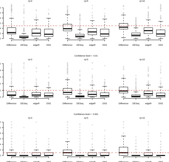
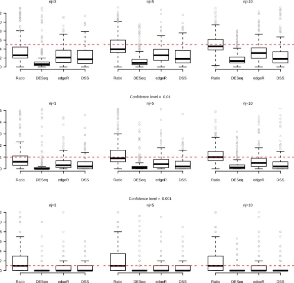
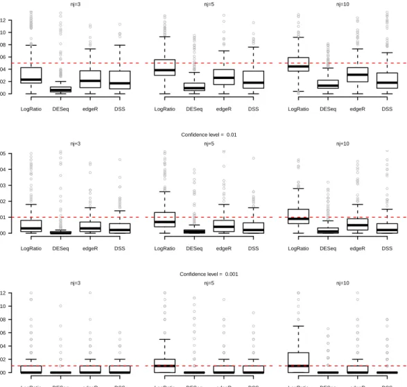
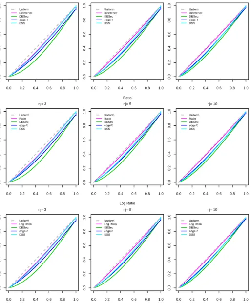
In particular, a statistical test procedure can be considered as well working and reliable if the empirical first type error (i.e. the proportion of times in which we reject the null-hypothesis for the genes that have been drawn as not differentially expressed) reaches the nominal value. Otherwise, if this does not occur, it means that the statistical distribution that has been considered as the reference one for the statistic under the null hypothesis is not correct.
We have compared the results of the three proposed statistical tests with the pro-cedures of Robinson et al. [2010], Anders and Huber [2010] and Wu et al. [2013], implemented in theRpackagesedgeR,DESeqandDSS, respectively.
36 5. A simulation study
5.1
Simulation A
In the first simulation study, we evaluated the capability of the proposed mix-ture model to estimate the variances of the genes as the number of components,K, increases. We also computed some conventional information criteria in order to select the optimal number of components. We have simulatedH = 100data-sets, each one drawing:
• p= 300genes, of which:
– 13 genes (= 100 genes) are differentially expressed (λi1 ̸=λi2) – 23 genes (= 200 genes) are not differentially expressed (λi1 =λi2)
• d= 2conditions
• nj = 5replicates for each condition;
• as regardsλij:
– for the 100 differentially expressed genesλi1 ∼U nif(0,250);
λi2 = λeϕii1 whereϕiis randomly drawn from aN(µ= 1, σ= 0.125)
– for the 200 non-differentially expressed genesλi1∼U nif(0,250)and
λi1 =λi2
• for all the genes, the αi (i = 1, . . . , p) are randomly drawn from a
U nif(0.5,600).
All the values for the parameters have been chosen to be consistent with the empirical situation.
On each data-set we fitted the proposed mixture model forK ranging from 1 to 6, and we have computed the relative distances in absolute values across the 100 data-sets between the estimated variancesV ar\(yijr)and the true onesV ar(yijr)
asKvaries, as follows:
distance(ijh)= |V ar(yijr)−V ar\(yijr) (h)
|
V ar(yijr)
(5.1) forj= 1,2,i= 1, . . . , pandh= 1, . . . , H; for the computation of the variances, since the number of replicates is limited we applied the factornj/(nj−1)to the
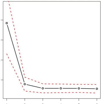
variance in (4.25), in order to obtain the corresponding correct estimator. Figure 5.1 shows the average distances and the standard error bands (mean±2·standard
5.1 Simulation A 37
error), and looking at the graph we could say that from K = 3components the gain of fitting more complex mixture models becomes irrelevant. In other terms, it seems thatK = 2 andK = 3components well describe the variability of the p
genes. 1 2 3 4 5 6 0.4 0.6 0.8 1.0
Number of mixture components
Relativ
e errors
Figure 5.1: Simulation A: Relative distances between the estimated variances and the true ones asKvaries. The dashed lines depict the standard error bands (mean±2·
se).
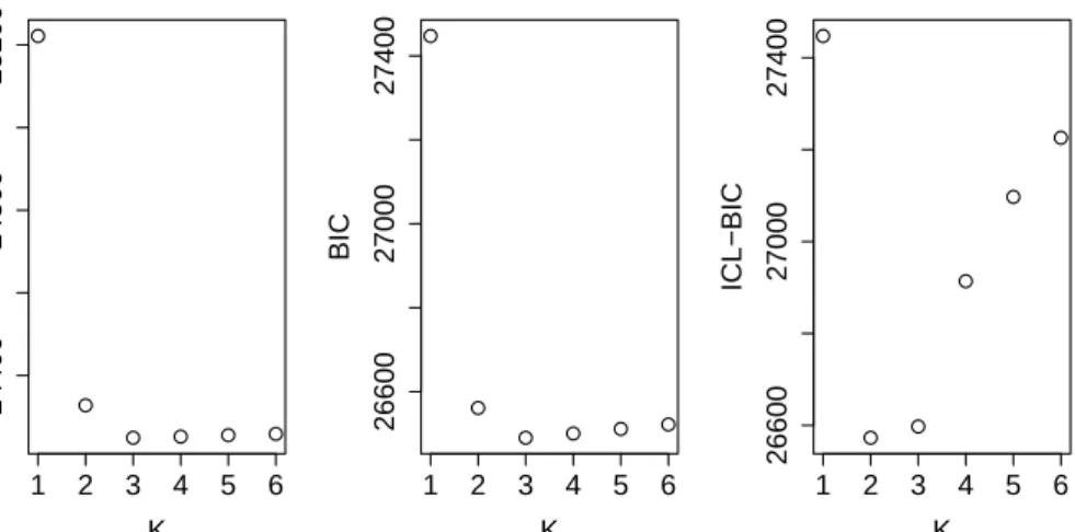
This insight is also confirmed by the information criteria. More specifi-cally, we have considered the Akaike’s Information Criterion (Akaike [1974]), AIC = −2 log maxL+ 2b, where b is the total number of required parameters and the more conservative Bayesian Information Criterion (Schwarz et al. [1978]), BIC =−2 log maxL+blogp. In addition, we have also computed the so-called Integrated Classification Likelihood Criterion (Biernacki et al. [2000]) that com-bines the BIC penalty term with the entropy of the posterior classification. As a result, ICL-BIC is characterized by a heavier penalty term and it tends to favor simpler models against mixture models with more components.
38 5. A simulation study
In Table 5.1 the number of times each criterion suggests a specific number of componentsK is shown. These results recommend that K = 3mixture compo-nents are enough to give a good description of the data.
Table 5.1: Simulation A: number of times each information criterion suggests a specific value forK.
K AIC BIC ICL-BIC
1 0 0 0 2 0 2 76 3 76 86 24 4 6 4 0 5 6 4 0 6 12 4 0
In Figure 5.2 the classic trend that we can observe for these information criteria is shown, and it is interesting to note that it is very similar to the one that describes the relative errors in the computation of the variances.
1 2 3 4 5 6 24400 24800 25200 K AIC 1 2 3 4 5 6 26600 27000 27400 K BIC 1 2 3 4 5 6 26600 27000 27400 K ICL−BIC
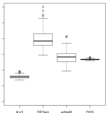
Figure 5.2: Simulation A: Information criteria asKvaries.
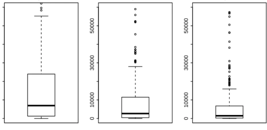
The relative errors of the variances have been computed also for the other already-known methods, using the Formula (5.1). In Figure 5.3 the boxplots that describe the distribution of these measures of bias for all the genes are presented. It is clear from this graph that the proposed method actually improves the estimation of the variances.