Statistical Methods to Account for Gene-Level Covariates in Normalization of High-Dimensional Read-Count Data

(1)

Utah State University Utah State University

DigitalCommons@USU

All Graduate Theses and Dissertations Graduate Studies

12-2018

Statistical Methods to Account for Gene-Level Covariates in

Normalization of High-Dimensional Read-Count Data

Lauren Holt Lenz

Utah State University

Follow this and additional works at: https://digitalcommons.usu.edu/etd

Part of the Statistics and Probability Commons Recommended Citation

Recommended Citation

Lenz, Lauren Holt, "Statistical Methods to Account for Gene-Level Covariates in Normalization of High-Dimensional Read-Count Data" (2018). All Graduate Theses and Dissertations. 7392.

https://digitalcommons.usu.edu/etd/7392

This Thesis is brought to you for free and open access by the Graduate Studies at DigitalCommons@USU. It has been accepted for inclusion in All Graduate Theses and Dissertations by an authorized administrator of DigitalCommons@USU. For more information, please contact [email protected].

(2)

STATISTICAL METHODS TO ACCOUNT FOR GENE-LEVEL COVARIATES IN NORMALIZATION OF HIGH-DIMENSIONAL READ-COUNT DATA

by

Lauren Holt Lenz

A thesis submitted in partial fulfillment of the requirements for the degree

of

MASTERS OF SCIENCE in

Statistics Approved:

John Stevens, Ph.D. Christopher Corcoran, Ph.D.

Major Professor Committee Member

Adele Cutler, Ph.D. Laurens H. Smith, Ph.D.

Committee Member Interim Vice President for Research and

Dean of the School of Graduate Studies UTAH STATE UNIVERSITY

Logan, Utah 2018

(3)

(4)

ii

ABSTRACT

Statistical Methods to Account for Gene-Level Covariates in Normalization of High-Dimensional Read-Count Data

by

Lauren Holt Lenz, Master of Science Utah State University, 2018 Major Professor: Dr. John R. Stevens

Department: Mathematics and Statistics

Normalization of RNA-Seq read-count data is a necessary pre-processing step in order to account for differences in read-count values due to non-expression re-lated variables. It is common in recent RNA-Seq normalization methods to also account for gene-level covariates, namely gene length in base pairs and GC-content. Here a colorectal cancer RNA-Seq read-count data set comprised of 30,220 genes and 378 samples is examined. Two of the normalization methods that account for gene length and GC-content, CQN and EDASeq, are extended to account for pro-tein coding status as a third gene-level covariate. The binary nature of propro-tein cod-ing status results in unique computation issues. The results of uscod-ing the normalized read counts from CQN, EDASeq, and four new normalization methods are used for differential expression analysis via the nonparametric Wilcoxon Rank-Sum Test as

well as the lme4 pipeline that produces per-gene models based on a negative

bino-mial distribution. The resulting differential expression results are compared for two genes of interest in colorectal cancer, APC and CTNNB1, both of the WNT signal-ing pathway.

(5)

iii

PUBLIC ABSTRACT

Statistical Methods to Account for Gene-Level Covariates in Normalization of High-Dimensional Read-Count Data

Lauren Holt Lenz

The goal of genetic-based cancer research is often to identify which genes be-have differently in cancerous and healthy tissue. This difference in behavior, re-ferred to as differential expression, may lead researchers to more targeted preven-tative care and treatment. One way to measure the expression of genes is though a process called RNA-Seq, that takes physical tissue samples and maps gene prod-ucts and fragments in the sample back to the gene that created it, resulting in a large read-count matrix with genes in the rows and a column for each sample. The read-counts for tumor and normal samples are then compared in a process called differential expression analysis. However, normalization of these read-counts is a necessary pre-processing step, in order to account for differences in the read-count values due to non-expression related variables. It is common in recent RNA-Seq normalization methods to also account for gene-level covariates, namely gene length in base pairs and GC-content, the proportion of bases in the gene that are Guanine and Cytosine.

Here a colorectal cancer RNA-Seq read-count data set comprised of 30,220 genes and 378 samples is examined. Two of the normalization methods that ac-count for gene length and GC-content, CQN and EDASeq, are extended to acac-count for protein coding status as a third gene-level covariate. The binary nature of pro-tein coding status results in unique computation issues. The results of using the normalized read counts from CQN, EDASeq, and four new normalization methods are used for differential expression analysis via the nonparametric Wilcoxon

(6)

Rank-iv

Sum Test as well as the lme4pipeline that produces per-gene models based on a

negative binomial distribution. The resulting differential expression results are com-pared for two genes of interest in colorectal cancer, APC and CTNNB1, both of the WNT signaling pathway.

(7)

v

ACKNOWLEDGMENTS

This research was made possible by funding from NIH grant award number 1R01CA16383-01A1 and from the Utah State University Department of Mathemat-ics and StatistMathemat-ics, as well as computing resources from the Center for High Perfor-mance Computing at the University of Utah. This project could not have been com-pleted with out the guidance and support of Dr. John Stevens.

(8)

vi

CONTENTS

Page

ABSTRACT . . . ii

PUBLIC ABSTRACT . . . iii

ACKNOWLEDGMENTS . . . v

LIST OF TABLES . . . viii

LIST OF FIGURES . . . x

CHAPTER 1. INTRODUCTION . . . 1

Motivating Example . . . 1

Motivating Data Set . . . 2

Covariate Data Set . . . 3

Covariate Sources . . . 4

Imputation of Covariate Values . . . 6

Differential Expression Analysis Methods . . . 12

2. EXISTING NORMALIZATION METHODS . . . 15

CQN . . . 15

Background . . . 15

Application to Motivating Data Set . . . 16

EDASeq . . . 20

Background . . . 20

Application to Motivating Data Set . . . 20

3. NEW NORMALIZATION METHODS . . . 25

Normalize Read-Counts Separately Based on Binary Covariate . . . 25

CQN . . . 26

EDASeq . . . 29

Compare Differential Expression Analysis Results . . . 33

Edit Existing Methods to Account for a Binary Covariate . . . 37

CQN . . . 38

EDASeq . . . 41

Compare Differential Expression Analysis Results . . . 50

4. COMPARISON OF RESULTS . . . 55

CQN Normalization and Variations . . . 55

EDASeq Normalization and Variations . . . 57

Genes of Interest . . . 61

APC . . . 61

CTNNB1 . . . 62

(9)

vii

REFERENCES . . . 66

(10)

viii

LIST OF TABLES

Table Page

0.1 Distribution of mean read-count per gene . . . 3

0.2 Summary of Covariates Pulled from Ensembl GRCh37 . . . 6

0.3 Wilcoxon Rank Sum Test results using CQN normalized read-counts 19

0.4 lme4 results using CQN offsets . . . 20

0.5 Wilcoxon Rank Sum Test results using EDASeq normalized

read-counts . . . 24

0.6 lme4 results using EDASeq offsets . . . 24

0.7 Wilcoxon Rank Sum Test results using CQN split on protein coding

status . . . 28

0.8 lme4 results using CQN split on protein coding status . . . 29

0.9 Wilcoxon Rank Sum Test results using EDASeq split on protein

coding status normalized read-counts . . . 32

0.10 lme4 results using EDASeq split on protein coding status offsets . . . 33

0.11 Wilcoxon Rank Sum Test results using CQN with jittered protein

coding status normalized read-counts . . . 41

0.12 lme4 results using CQN with jittered protein coding status offsets . . 41

0.13 Wilcoxon Rank Sum Test results using EDASeq normalizing for

GC-content then protein coding status . . . 47

0.14 Wilcoxon Rank Sum Test results using EDASeq normalizing for

protein coding status then GC-content . . . 48

0.15 Comparing the calls of differential expression from the Wilcoxon Rank Sum test on all genes when using EDASeq offsets on three

covariates . . . 48

0.16 Comparing the calls of differential expression from the Wilcoxon Rank Sum test on filtered genes when using EDASeq offsets on three

(11)

ix

0.17 lme4 results using EDASeq normalizing for GC-content then protein

coding status . . . 49

0.18 lme4 results using EDASeq normalizing for protein coding status

then GC-content . . . 49

0.19 Comparing the calls of differential expression from thelme4 pipeline

on all genes when using EDASeq offsets on three covariates . . . 50

0.20 Comparing the calls of differential expression from thelme4 pipeline

(12)

x

LIST OF FIGURES

Figure Page

0.1 Distribution of mean read-count per-gene . . . 3

0.2 Distributions of Covariates Pulled from Ensembl GRCh37 . . . 5

0.3 Example of imputation robustness test - true vs. imputed values . . . 7

0.4 Example of imputation and linear adjustment robustness test -

GC-content . . . 8

0.5 Example of imputation and linear adjustment robustness test - gene

length . . . 9

0.6 Comparison of imputed and adjusted covariate values - GC-content . 10

0.7 Comparison of imputed and adjusted covariate values - gene length . 11

0.8 Comparison of imputed and adjusted covariate values - log(gene

length) . . . 12

0.9 Distribution of CQN offsets when normalizing for GC-content . . . . 16

0.10 Systematic effects for CQN with all genes and GC-content . . . 17

0.11 Systematic effects for CQN with filtered genes and GC-content . . . . 17

0.12 Distribution of EDASeq offsets when normalizing for GC-content . . 21

0.13 Read-count mean variance plot for over-dispersion . . . 21

0.14 Comparison of lowess regression on raw read-counts and normalized

read-counts - All Genes . . . 22

read-counts - Filtered Genes . . . 23

0.16 Distribution of CQN offsets when split on protein coding status prior

to normalizing for GC-content . . . 26

0.17 Systematic effects for CQN with all genes split on protein coding

(13)

xi 0.18 Systematic effects for CQN with filtered genes split on protein

cod-ing status . . . 28

0.19 Distribution of EDASeq offsets when split on protein coding status

prior to normalizing for GC-content . . . 30

read-counts - All Genes Split on Protein Coding Status . . . 31

read-counts - Filtered Genes Split on Protein Coding Status . . . 32

0.22 Comparison of results using CQN with GC-content and CQN split

on protein coding status . . . 34

0.23 Comparison of results using EDASeq with GC-content and EDASeq

split on protein coding status . . . 35

0.24 Comparing Mean Squared Differences from lme4log2 fold change

values . . . 37

0.25 Distribution of CQN offsets when normalizing with jittered protein

0.26 Systematic effects for CQN with all genes and jittered protein coding

status . . . 40

0.27 Systematic effects for CQN with filtered genes and jittered protein

0.28 Distribution of EDASeq offsets when normalizing for GC-content

then protein coding status . . . 42

0.29 Distribution of EDASeq offsets when normalizing for protein coding

status then GC-content . . . 42

0.30 Comparison of lowess regression on all genes raw read-counts and

read-counts normalized with GC-content then protein coding status . 44

0.31 Comparison of lowess regression on all genes raw read-counts and

read-counts normalized with protein coding status then GC-content . 45

0.32 Comparison of lowess regression on filtered genes’ raw read-counts and read-counts normalized with GC-content then protein coding

(14)

xii 0.33 Comparison of lowess regression on filtered genes raw read-counts

and read-counts normalized with protein coding status then

GC-content . . . 47

0.34 Comparing the log2 fold changes from the lme4 pipeline when using

EDASeq offsets on three covariates . . . 49

0.35 Comparison of results using CQN with GC-content and CQN with

jittered protein coding status . . . 51

with GC-content, then protein coding status . . . 53

with protein coding status, then GC-content . . . 54

0.38 Comparison of lme4results using CQN variations . . . 56

0.39 Comparison of Wilcoxon Rank Sum Test results using CQN variations 57

0.40 Comparison of lme4results using EDASeq variations . . . 59

0.41 Comparison of Wilcoxon Rank Sum Test results using EDASeq

variations . . . 60

0.42 Comparison of All Test Results for APC . . . 62

0.43 Comparison of All Test Results for CTNNB1 . . . 63

0.44 Comparison of log(gene length) and GC-content values for all genes . 65

0.45 Comparison of log(gene length) and GC-content values for filtered

(15)

CHAPTER 1 INTRODUCTION

RNA-Seq technology takes mRNA from a biological sample and maps the mRNA present to a reference genome (“Illumina: RNA Sequencing Data Analysis Solutions” San Deigo, California, Wang, Gerstein, and Snyder (2009)). The result-ing data consists of a count of mRNA fragments (“reads”) whose sequences map to each gene in each sample. These read-counts represent measurements of the ex-pression levels of the genome’s genes in each biological sample. Traditionally, re-searchers are interested in identifying differentially expressed genes whose expres-sion levels change systematically between groups, such as tumor vs. normal in a cancer study.

When using read-count data to identify differentially expressed genes, nor-malization is a necessary pre-processing step. Nornor-malization accounts for differ-ences that cause some read-counts to be higher than others due to non-expression related variables such as differences in the size of biological samples, the length of each gene, and machine calibrations. Classical normalization approaches deal with reads per kilo-million, or RPKM, which normalizes by taking into account the to-tal number of reads each sample has across all genes, commonly referred to as the sequencing depth.

Motivating Example

RNA-Seq was run using the Illumina pipeline (“Illumina: RNA Sequencing Data Analysis Solutions” San Deigo, California) on 378 samples from 209 individu-als. These 378 samples consist of 187 normal (non-tumor) samples and 191 tumor samples, of which there are 169 pairs and 40 unpaired samples. The RNA-Seq

(16)

pro-Introduction 2 cess resulted in a read-count for each sample at each of the 30,220 genes, of which 17,462 (57.78%) are protein coding and 12,758 (42.22%) are non-protein coding (Slattery et al. 2017).

The original team examining this read-count data set at the University of

Utah used the DESeq2 pipeline (Love, Huber, and Anders 2014) and the Wilcoxon

Rank Sum test (Hothorn et al. 2008) for differential expression analysis between tumor and normal samples; however, some genes did not show the expression dif-ferences expected. In colorectal cancer the WNT signaling pathway is studied ex-tensively and fairly well understood (Suzuki et al. 2004, Nagase and Nakamura (1993), Segditsas and Tomlinson (2006)). The WNT signaling pathway gene APC

is believed to be down-regulated in colorectal cancer (Nagase and Nakamura 1993), and the gene CTNNB1 is expected to be up-regulated in colorectal cancer (Suzuki et al. 2004). The Wilcoxon Rank Sum test run with standard RPKM normaliza-tion on this data set showed that APC was not significantly differentially expressed. This “flip” in expression caused the original researchers to question the validity of the other differential expression analysis results and raises this project’s research question: Does accounting for gene-level covariates in pre-processing normalization of high-dimensional RNA-Seq read-count data improve the accuracy of differential expression analysis?

Motivating Data Set

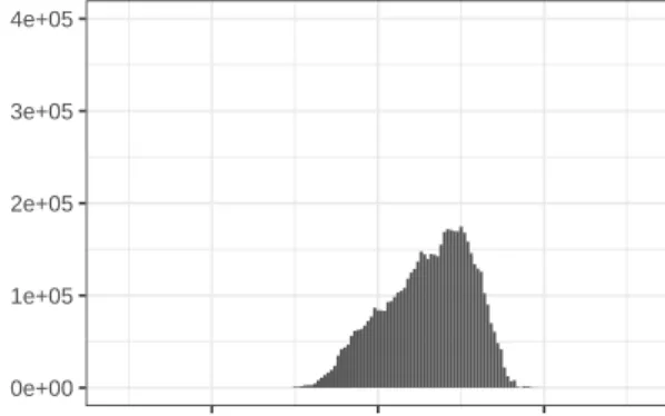
The read-counts in this data set have a very large spread. Figure 0.1 shows the mean read-count across all samples for each gene, on the true and log scales. The majority of genes have a mean read count across samples of less than 1,000, and only 77 of the 30,220 genes have mean read counts higher than 1,500. Table 0.1 shows summary statistics for the mean read-count across samples for each gene. Notice the huge difference in the mean and median of the genes’ mean read-counts.

(17)

Introduction 3

Table 0.1: Distribution of mean read-count per gene

Minimum 1st Quartile Median Mean 3rd Quartile Maximum

0.5 2.0 9.2 193.4 47.8 719969.7

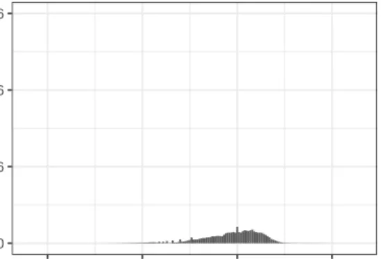
Figure 0.1: Distribution of mean read-count per-gene

0 10000 20000 30000

0e+00 2e+05 4e+05 6e+05 Mean read−count count 0 1000 2000 0 5 10 Mean log(read−count) count

Distribution of Mean Read−Count Across Samples

A filtered data set was also produced by filtering out the “non-expressed” genes. A mean read-count threshold of 10 was set at the suggestion of Risso et al. (2011), and all genes with a mean-read count across all samples of less then 10 were

labeled as “non-expressed” and were removed from the data set, leaving 14,715 genes, 12,618 of which are protein coding (85.75%). All covariate calculations ex-plained below were performed on all genes, with this filter applied before normaliza-tion.

Covariate Data Set

Gene-level covariates previously used in read-count normalization are gene length in bases, and GC-content, the proportion of bases in a gene sequence that are Guanine and Cytosine as opposed to Adenine and Thymine (Hansen, Irizarry, and Wu 2012). Because RNA-Seq maps gene fragments and gene products back to

(18)

Introduction 4 the gene that produced them, longer genes will have higher read-counts and expres-sion levels, leading to more significance in differential expresexpres-sion analysis (Risso et al. 2011). When designing a new normalization method, Risso et al. (2011) stated “GC-rich and GC-poor fragments tend to be underrepresented in RNA-Seq” (Risso et al. 2011), and it has been shown that bias related to GC-content leads to false positives in downstream differential expression analysis (Hansen, Irizarry, and Wu 2012).

Ideally, researchers would be aware of normalization methods that account for gene-level covariates while designing their experiment, allowing the sequences used in the initial RNA-Seq process to be used to calculate both GC-content and gene length. However, in cases like this motivating example where the sequences used in the RNA-Seq process that provided the read-counts are unavailable, the researcher attempting to use a method that requires per-gene covariate information must calculate covariates from suitable gene sequences that are as close to what were used in RNA-Seq as possible.

Covariate Sources

Several options for pulling gene sequences are available for free online, includ-ing the University of California Santa Cruz Genome Browser (Kent et al. 2002), and the Ensembl Database website (Zerbino et al. 2017). The company that pro-duced the materials used in the original RNA-Seq process may also provide refer-ence sequrefer-ences online.

Gene sequences used for this data set’s RNA-Seq process were pulled from the GRCh37 build of the human genome data base via the UCSC website, and aligned using novoalign v2.08.01. (Slattery et al. 2017). Since those sequences were not available for my use, I attempted to pull the sequences from the data base. The UCSC Gene Browser allows a user to pull transcript sequences corresponding to an

(19)

Introduction 5 Ensembl gene ID, but not entire gene sequences. Genes are typically made up of several transcripts, and some may overlap or leave gaps in the gene sequence. Be-cause I am not confident in my ability to piece together a gene sequence from tran-scripts, I instead pulled gene sequences from the Ensembl database, build GRCh37 (Zerbino et al. 2017). While these sequences are not the exact ones used in the

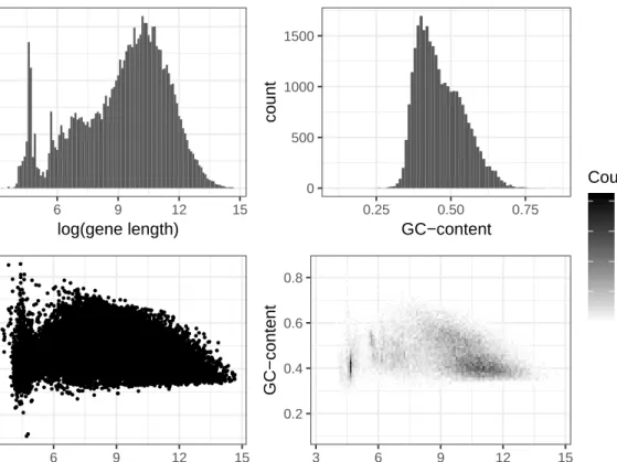
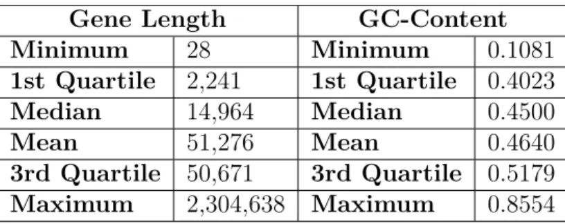
orig-inal RNA-Seq process, I expect that they are reasonably close, as they are from the same data base build that was accessed by the original researchers (Slattery et al. 2017). Graphical displays of the distributions of gene lengths and GC-content val-ues are shown in Figure 0.2, with summaries of the distributions shown in Table 0.2.

Figure 0.2: Distributions of Covariates Pulled from Ensembl GRCh37

0 200 400 600 3 6 9 12 15 log(gene length) count 0 500 1000 1500 0.25 0.50 0.75 GC−content count 0.2 0.4 0.6 0.8 3 6 9 12 15 log(gene length) GC−content 0.2 0.4 0.6 0.8 3 6 9 12 15 log(gene length) GC−content 0 20 40 60 80 Count

(20)

Introduction 6

Table 0.2: Summary of Covariates Pulled from Ensembl GRCh37

Gene Length GC-Content

Minimum 28 Minimum 0.1081 1st Quartile 2,241 1st Quartile 0.4023 Median 14,964 Median 0.4500 Mean 51,276 Mean 0.4640 3rd Quartile 50,671 3rd Quartile 0.5179 Maximum 2,304,638 Maximum 0.8554

Even when pulling from the same genome database build as the original re-searchers, 1,885 of the 30,220 (6.24%) Ensembl gene IDs were not in the database, resulting in missing gene lengths and GC-content values for those genes. Of the 1,885 genes not in the database, 1,852 are non-protein coding genes (98.25%), and 1,365 (72.41%) have mean read-count values less than 10, and would be classified as non-expressed.

Since the read-count data set had no missing expression values for these 1,885 genes, it would be unwise to remove them from the data set and not include them in differential expression analysis. However, in order to include these genes in meth-ods that consider gene-level covariates, the missing gene length and GC-content values must be imputed.

Imputation of Covariate Values

The packagemissForest (Stekhoven 2013) was used to impute missing gene

length and GC-content values. Prior to imputing the 1,885 missing values, the

accu-racy of missForest imputation needed to be established. To do so, a random

sam-ple of 5,000 genes was taken from the 28,335 known genes, their covariates were re-moved from the data set, and then the 5,000 “missing” values were imputed based on the gene length and GC-content values for the 23,335 remaining known genes, and read count values for all 28,335 genes.

(21)

estab-Introduction 7

lish that the accuracy of missForest was not a result of the 5,000 genes randomly

selected. Imputed and true gene length and GC-content values were plotted for a

visual measure of the accuracy and robustness of missForest imputation. All five

replicates showed very similar patterns, Figure 0.3 shows one of these robustness test replicates.

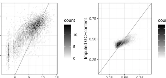
Figure 0.3: Example of imputation robustness test - true vs. imputed values

8 10 12

6 9 12 15

True log(gene length)

Imputed log(gene length) 0 5 10 count 0.25 0.50 0.75 0.25 0.50 0.75 True GC−content Imputed GC−content 0 10 20 30 40 50 count

Note in Figure 0.3, the log-scale gene length plots show some bi-modality in the true gene length values that is not seen in the imputed values. Also note how both the imputed gene length values and the imputed GC-content values appear to follow a fairly linear trend, but the slopes of those linear trends are not one. For this reason I decided to apply a linear model adjustment to each covariate to im-prove imputation accuracy.

To calculate and test linear models, I took each of the five replicates men-tioned above and randomly split them into two groups, training and testing. Each of the five training sets were use to create a linear model where the imputed value depends on the true value, and then the corresponding test set were used to vi-sualize the accuracy of the linear models. Figure 0.4 shows true vs. imputed

(22)

GC-Introduction 8 content and true vs. imputed-then-adjusted GC-content. The application of the linear model adjustment results in adjusted values that are much closer to the true values on average.

Next the linear models themselves were examined, and because all five models are very similar, the mean of the intercept and the GC-content coefficient were used to create a single linear model adjustment to apply to the imputed GC-content val-ues of the 1,885 missing genes.

The same process was followed for a linear model adjustment for gene lengths on the log scale. As seen in Figure 0.5, the linear model adjustment is less beneficial for log-scale gene lengths than for GC-content, but it is an improve-ment, so the linear model adjustment was applied to the 1,885 imputed values.

Figure 0.4: Example of imputation and linear adjustment robustness test - GC-content

0.25 0.50 0.75 0.25 0.50 0.75 True GC−content Imputed GC−content 0 10 20 30 40 50 count 0.25 0.50 0.75 0.25 0.50 0.75 True GC−content Ajusted GC−content ₀ 5 10 15 20 count

(23)

Introduction 9

Figure 0.5: Example of imputation and linear adjustment robustness test - gene length

8 10 12

6 9 12 15

Imputed log(gene length) 0 5 10 count 5.0 7.5 10.0 12.5 6 9 12 15

Adjusted log(gene length) 0 2 4 6 count

After establishing the validity and robustness of missForest imputation

and a linear model was constructed to increase accuracy, the missing gene length and GC-content values were imputed using the covariates from the 28,335 known genes and the read counts for all 30,220 genes. The linear model adjustments for gene length and GC-content were applied to the 1,885 imputed values, resulting in the covariate data set used throughout the rest of this thesis. Distributions of known, imputed, and adjusted covariates are seen in Figures 0.6, 0.7, and 0.8.

(24)

Introduction 10

Figure 0.6: Comparison of imputed and adjusted covariate values - GC-content

0 500 1000 1500

0.25 0.50 0.75 1.00

Known and imputed GC−content

count 0 500 1000 1500 0.25 0.50 0.75 1.00

Known and adjusted GC−content

count 0 100 200 300 0.25 0.50 0.75 1.00 Imputed GC−content count 0 100 200 300 0.25 0.50 0.75 1.00 Adjusted GC−content count

(25)

Introduction 11

Figure 0.7: Comparison of imputed and adjusted covariate values - gene length

0 2500 5000 7500 10000

0e+00 1e+06 2e+06 3e+06

Known and imputed gene length

count 0 2500 5000 7500 10000

0e+00 1e+06 2e+06 3e+06

Known and adjusted gene length

count

0 200 400

0e+00 1e+05 2e+05 3e+05

Imputed gene length

count

0 200 400

0e+00 1e+05 2e+05 3e+05

Adjusted gene length

(26)

Introduction 12

Figure 0.8: Comparison of imputed and adjusted covariate values - log(gene length)

0 500 1000 1500

4 8 12

Known and imputed log(gene length)

count 0 500 1000 1500 4 8 12

Known and adjusted log(gene length)

count 0 50 100 150 200 4 8 12

Imputed log(gene length)

count 0 50 100 150 200 4 8 12

Adjusted log(gene length)

count

Differential Expression Analysis Methods

Several methods for determining the differential expression of genes are avail-able, including methods designed especially for RNA-Seq data. The University of

Utah researchers used the DESeq2 pipeline (Love, Huber, and Anders 2014) and the

Wilcoxon Rank Sum test, but this project will focus on the use of the lme4pipeline

and the Wilcoxon Rank Sum test from the R package coin(Hothorn et al. 2008).

The lme4 pipeline (Bates et al. 2015) is most appropriate for this data set because

(27)

Introduction 13 sample ID random effect, when producing per-gene models. Other, computationally

faster, differential expression analysis methods including DESeq2 (Love, Huber, and

Anders 2014) and edgeR (Robinson, McCarthy, and Smyth 2010) account for fixed

effects but have no way to account for the sample ID random effect.

LetNi be the total number of mRNA fragments in sample i, pi be the

prob-ability that a fragment maps to a given gene in samplei, and Ri be the number of

fragments in sample i that map back to the given gene. Then the lme4pipeline

al-lows Ri ∼N egativeBinomial(µi, σ2_i)where µi =Nipi so log (E[Ri]) = log Ni+ log

pi. The default “offset” (log Ni) in this model can be replaced by a normalizing

off-set value, and the link function (log pi) is set equal to a linear model such as log

pi =µ+ (effect of samplei’s treatment group) + (effect of sample i’s subject). All of the normalization methods discussed in Chapters 2 and 3 return both offsets and normalized read-counts, which can then be passed to differential expres-sion analysis methods. There is some debate on whether offsets or normalized read-counts are better to use overall (Risso et al. 2011), so in this project I followed the published vignettes for the normalization methods. The Wilcoxon Rank Sum test

takes normalized-read counts, but the lme4 pipeline takes raw read-counts and the

offset values.

The documentation forlme4 describes the offset as a way to “specify an a

priori known component to be included in the linear predictor during [the] fitting [of per-gene models]”, which essentially means that the offset values are added into the linear mixed-effect model to adjust the inputted raw read-counts for

normal-ization (Bates et al. 2015). Mathematically, this is seen as follows, let Y represent

the response (gene expression values), n is the dimension of the response vector,

W is a diagonal matrix of known prior weights,β is a p-dimensional coefficient

vector,X is an n ×pmodel matrix, o is a vector of known prior offset terms, and

(28)

Introduction 14 Y ∼N(Xβ+o, σ2_W−1₎ _{(Bates et al. 2015).}

(29)

15

CHAPTER 2

EXISTING NORMALIZATION METHODS

In this thesis project I will be using two normalization methods that use gene-level covariates: Conditional Quantile Normalization (CQN) (Hansen, Irizarry, and Wu 2012) and Exploratory Data Analysis and Normalization for RNA-Seq (EDASeq) (Risso et al. 2011). Both methods are published as R packages by

Bio-conductor (Huber et al. 2015) and use gene length and GC-content as gene-level covariates. The results of these normalization methods include normalized read-counts that are used in the non-parametric Wilcoxon Rank Sum Test (Hothorn et

al. 2008), and offsets that are used in the lme4pipeline to produce per-gene models

(Bates et al. 2015).

CQN Background

Hansen, Irizarry, and Wu (2012) found that GC-content has a strong sample-specific effect on RNA-Seq read-counts that can lead to false positives in differential expression analysis. This motivated the new conditional quantile normalization al-gorithm that removes systematic bias introduced by covariates, as well as global distortions caused by differences in sequencing depths. As described by Risso et al. (2011),

“[The CQN] procedure, which combines both within and between lane [or sample] normalization and is based on a Poisson model for read counts. Lane-specific systematic biases, such as GC-content and length effects, are incorporated as smooth functions using natural cubic splines

(30)

Existing Normalization Methods 16 and estimated using robust quantile regression. In order to account for

distributional differences between lanes, a full-quantile normalization procedure is adopted, in the spirit of that considered in Bullard et al. (2010). The main advantage of this approach is that it is lane-specific,

i.e., it works independently in each lane, aiming at removing the bias rather than equalizing it across lanes. Modeling simultaneously GC-content and length (and in principle other sources of bias) leads to a flexible normalization method.” (Risso et al. 2011)

Application to Motivating Data Set

Following the published vignette for the cqnpackage (Hansen, Irizarry,

and Wu 2012), CQN was run on all genes, as well as the filtered subset. The resulting object of class “cqn” contains offsets that can be used to calculate normalized read-count values. The distribution of those offsets is visual-ized in Figure 0.9. The full and filtered data sets produce offsets with the same general distribution, a fairly unimodal, slightly left-skewed, distribution.

Figure 0.9: Distribution of CQN offsets when normalizing for GC-content

0e+00 1e+05 2e+05 3e+05 4e+05 −5 0 5 Offset value count All Genes 0e+00 1e+05 2e+05 3e+05 4e+05 −5 0 5 Offset value count Filtered Genes

The object of class “cqn” can be passed to the functioncqnplot which

(31)

system-Existing Normalization Methods 17

atic effects are (1) whatever covariate passed tocqn and (2) the gene lengths

passed to cqn. The lines on the resulting plots show estimated beta-spline

de-pendence of counts on the systematic effect, with the systematic effect on the x-axis (with the knots used to fit the beta splines shown as additional ticks), and the QR fit on the y-axis (Love 2016). The cqnplots for the full data set are seen in Figure 0.10, and the cqnplots for the filtered data set are in Figure 0.11.

Figure 0.10: Systematic effects for CQN with all genes and GC-content

Figure 0.11: Systematic effects for CQN with filtered genes and GC-content

Although Figures 0.10 and 0.11 look to be identical, there are very slight vari-ations in the splines due to the filtering of the read-counts matrix. CQN normal-ization does not require filtering out “non-expressed” genes (where EDASeq highly

(32)

Existing Normalization Methods 18 recommends it), likely because the non-expressed genes have very little impact on the overall normalization of the read-counts, which is supported by the similarity of Figures 0.10 and 0.11. The spread of the splines in both the GC-content and gene lengths plots suggest that there is quite a bit of variability between samples in the estimated splines (Love 2016).

According to Love, a typical cqn plot for GC-content would have an “upside-down U” shape, indicating that the low and high GC-content fragments are under-represented (Love 2016). Figures 0.10 and 0.11 appear to have no distinct upside-down U shape in the GC-content splines, suggesting that the genes with more ex-treme GC-content are not as underrepresented as we would have expected. There is, however, an overall positive slope on the far left-hand side of the GC-content plot, representing small GC-content values, so there may be evidence that genes with low GC-content are actually underrepresented. Love also describes the typical pattern for the gene lengths splines to show more counts for longer genes (Love 2016). In the gene lengths plots in Figures 0.10 and 0.11, however, there is no overall positive slope, suggesting that there may not be more counts for longer genes in our data set.

Wilcoxon Rank Sum Test

The normalized read counts (on thelog2 scale) from CQN were used in the

Wilcoxon Rank Sum Test function wilcox_test from the package coin (Hothorn et

al. 2008). The log2 scale was used so that the resulting object would contain an

“estimate” value that estimates the log2 fold change comparing tumor samples to

normal samples (i.e. a negative estimate would mean that gene is down-regulated in tumor samples, with significance depending on the FDR corrected p-value).

A combination of the resultinglog2 fold change values and the FDR corrected

(33)

Existing Normalization Methods 19 gene. Results are summarized in Table 0.3.

Table 0.3: Wilcoxon Rank Sum Test results using CQN normalized read-counts

Wilcoxon Rank Sum

Test Results Failed

Down Regulated Not Significant Up Regulated All Genes: 30,220 0 (0%) 7,738 (25.61%) 12,522 (41.44%) 9,960 (32.96%) Filtered Genes: 14,715 0 (0%) 5,179 (35.20%) 3,559 (24.19%) 5,977 (40.62%)

Filtering the genes prior to normalization has a large effect on the propor-tion of genes identified as significant. Filtering out 15,505 “non-expressed” genes removed nearly 10,000 genes from the not-significantly-differentially-expressed cate-gory, resulting in a higher percentage of the remaining 14,715 genes being identified as significantly differentially expressed.

lme4 Models

The lme4R package (Bates et al. 2015) available from CRAN produces

per-gene models that account for fixed and random effects, while assuming read-counts follow a negative binomial distribution. The offsets from CQN normalization

were passed into the lme4 pipeline following the lme4 vignette. lme4 is fairly

computationally intensive, so models were run using the University of Utah Center

for High Performance Computing (Barton 2016). The output from the glmer.nb

function in thelme4 pipeline contains fixed-effect estimates, which are equivalent

tolog2 fold change values, and raw p-values, from which FDR corrected p-values

were calculated. As in the Wilcoxon Rank Sum Test, the sign of the log2 fold

change and the FDR corrected p-value were used to determine the significance and dysregulation (up or down) of each gene. Results are summarized in Table 0.4.

(34)

Existing Normalization Methods 20

Table 0.4: lme4 results using CQN offsets lme4

Down Regulated Not Significant Up Regulated All Genes: 30,220 310 (1.03%) 7, 602 (25.16%) 10,540 (34.88%) 11,768 (38.94%) Filtered Genes: 14,715 38 (0.265) 4,903 (33.32%) 3,245 (22.05%) 6,529 (44.37%)

Comparing the results from lme4 (Table 0.4) and the Wilcoxon Rank Sum

test (Table 0.3),lme4 tends to identify more significantly up-regulated genes, in

both the full and filtered data sets. This is likely because lme4 accounts for

variabil-ity due to a subject random effect, making the test for the tumor fixed effect more powerful due to there being less unexplained variability.

EDASeq Background

In their original 2011 BMC Bioinformatics paper, Risso et al. (2011) break

down sources of bias in RNA-Seq read counts into two main categories: within-lane gene-specific effects, including GC-content and gene length, and between-lane dis-tributional differences, including sequencing depth. Risso et al. (2011) also states that normalizing by “scaling counts by gene length is not sufficient for removing [within-lane] bias”, which is similar to what is done in the classic RPKM normaliza-tion method. Therefore by normalizing within-lane and then between-lane, EDASeq claims to lead to more accurate gene expression levels, “making statistical inference of differential expression less prone to false discoveries” (Risso et al. 2011).

Application to Motivating Data Set

Following the published vignette for the EDASeq package (Risso et al.

2011), EDASeq normalization was run on all genes, as well as the filtered subset. The distribution of the resulting offsets are shown in Figure 0.12.

(35)

Figure 0.12: Distribution of EDASeq offsets when normalizing for GC-content

0e+00 1e+06 2e+06 3e+06 −10 −5 0 5 Offset value count All Genes 0e+00 1e+06 2e+06 3e+06 −10 −5 0 5 Offset value count Filtered Genes

The distribution of offsets produced by EDASeq normalization for the full data set has a very large spike at zero that is not seen in the filtered data set. This suggests that the expressed” genes filtered out of the data set were likely “non-expressed” across both tumor and normal samples.

In the EDASeq package there is more of a focus on exploratory analysis than in the CQN package, including some useful diagnostic plots. The most useful diagnostic plot for this data set is the over-dispersion plot, seen in Figure 0.13.

Figure 0.13: Read-count mean variance plot for over-dispersion

0 5 10 15 0 5 10 15 20 25 mean v ar iance All Genes 0 5 10 15 0 5 10 15 20 25 mean v ar iance Filtered Genes

Figure 0.13 shows the mean and variance of read-counts within each sample. If the mean and variance were equal (following the black line of equality), then

(36)

Existing Normalization Methods 22 a Poisson distribution would be appropriate for the data set. The red line shows a lowess fit for the mean-variance relationship, that in both the filtered and un-filtered data sets are significantly different than the black line of equality. This suggests that a Poisson distribution is inappropriate, and that a negative binomial distribution for the read-counts should be used. This is another reason why the

lme4 pipeline for differential expression analysis is most appropriate, as it allows

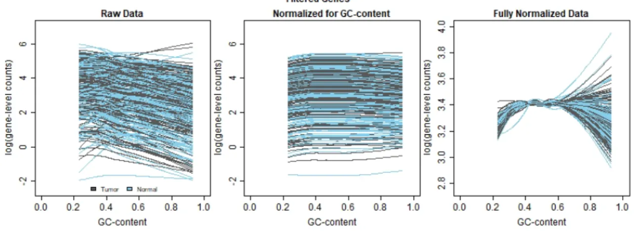
the read-counts to follow a negative binomial distribution (Bates et al. 2015). EDASeq also produces bias plots on normalized data. These bias plots (Figures 0.14 and 0.15) show lowess regression curves, one for each

sam-ple, with GC-content on the x-axis and log(gene-level counts) on the y-axis.

Figure 0.14: Comparison of lowess regression on raw counts and normalized read-counts - All Genes

The raw data plotted in Figure 0.14 shows quite a bit of spread, with more of the overall upside-down U shape anticipated in the typical cqn plot (Love 2016). The data normalized for GC-content smooths out some of the variation in the mid-level GC-content, and the dramatic change comes from accounting for sequencing depth, the between lane normalization. The fully normalized data plot is very com-pressed toward the center of the GC-content distribution, which matches the inter-pretation that genes with extreme GC-content values may be underrepresented in

(37)

Existing Normalization Methods 23 read-counts, and genes with moderate GC-content values may be over-represented.

Figure 0.15: Comparison of lowess regression on raw counts and normalized read-counts - Filtered Genes

Notice the difference in scale between the first two and third plots of Figure 0.15, as well as the difference from the all genes plot (Figure 0.14) to the filtered genes plot (Figure 0.15). There is much less of an upside down U shape in the fil-tered raw data than in the complete raw data. Likely this means that many of the genes with extreme GC-content values and lower read-counts were filtered out. As in the all genes plot, normalizing for GC-content appears to remove some of the variation seen in the raw data. The fully normalized data plot has a very narrow range, even on the far high range of GC-content with the most vertical spread, which means EDASeq on filtered data has removed much of the variation in the distribution of read-counts across samples.

Wilcoxon Rank Sum Test

The Wilcoxon Rank Sum tests were run in the same way for EDASeq as for CQN (described above). Results of the Wilcoxon Rank Sum test run on EDASeq normalized read-counts are summarized in Table 0.5, with FDR controlled at 0.05.

(38)

Table 0.5: Wilcoxon Rank Sum Test results using EDASeq normalized read-counts Wilcoxon Rank Sum

Down Regulated Not Significant Up Regulated All Genes: 30,220 1 (0.003 %) 9,707 (32.12%) 11,447 (37.89%) 9,065 (30.00%) Filtered Genes: 14,715 2 (0.014%) 5,352 (36.37%) 3,447 (23.43%) 5,914 (40.19 %)

It is interesting to note that the CQN normalized read-counts produced no NA values (failed tests), but here there was one failed test in the full data set, and two failed tests in the filtered data set (compare Tables 0.3 and 0.5). These failed tests were accompanied by the warning “The conditional covariance matrix has zero diagonal elements”.

lme4 Models

The lme4pipeline was handled the same way for EDASeq as for CQN

(described above). Results of the per-gene models are summarized in Table 0.6.

Table 0.6: lme4 results using EDASeq offsets lme4

Down Regulated Not Significant Up Regulated All Genes: 30,220 544 (1.80%) 9,310 (30.81%) 11,033 (36.51%) 9,333 (30.88%) Filtered Genes: 14,715 437 (2.97%) 5,111 (34.73%) 3,404 (23.13%) 5,736 (39.16%)

The percentage of failed models is slightly higher when using EDASeq offsets than when using CQN offsets for all variations of both normalization methods. An-other point of interest is that filtering out non-expressed genes is explicitly recom-mended in the EDASeq vignette, but not in the CQN vignette, so here focus should be placed on the results of the filtered data set (Risso et al. 2011).

(39)

25

CHAPTER 3

NEW NORMALIZATION METHODS

Both CQN and EDASeq normalization methods only account for gene length and GC-content. While the original Hansen, Irizarry, and Wu (2012) paper intro-ducing CQN states that the CQN model “permits the inclusion of other [covari-ates]: for example, mappability or more elaborate models of sequence effects”, no published examples of using CQN with any covariates other than gene length and GC-content could be found. And, for both CQN and EDASeq, trying to run the pipeline as-is with gene length and protein coding status causes fatal computational errors to occur. For this reason I began looking for a solution to account for protein coding status, a binary covariate, as well as gene length and GC-content in normal-ization.

Normalize Read-Counts Separately Based on Binary Covariate

When the original issue of APC’s unexpected expression was found by the University of Utah researchers (recall “Motivating Example” section in Chapter 1), it was suggested that perhaps only the protein coding genes should be examined for differential expression. This would mean that the non-protein coding genes be-ing included in the analysis changed the distribution of read-counts enough to alter the results of the test. So, if the distributions of read-counts for protein and non-protein coding genes are so different, perhaps they should be normalized separately. This would allow for the protein coding genes’ read-counts to not be affected by the read-counts for the non-protein coding genes, without throwing out the data for the non-protein coding genes.

(40)

New Normalization Methods 26

CQN

Application to Motivating Data Set

The distribution of offset values when running CQN normalization on protein coding and non-protein coding genes separately is shown in Figure 0.16.

Figure 0.16: Distribution of CQN offsets when split on protein coding status prior to normalizing for GC-content

0e+00 1e+05 2e+05 3e+05 −5 0 5 Offset value count

All Protein Coding Genes

Filtered Protein Coding Genes

All Non−protein Coding Genes

Filtered Non−protein Coding Genes

All four data sets in Figure 0.16 appear to have fairly normally distributed off-sets, with the non-protein coding genes’ offsets being centered further to the right. This difference in the distribution of offsets suggests that the distribution of read-counts for protein and non-protein coding genes are different.

(41)

New Normalization Methods 27 Figures 0.17 and 0.18, respectively. The difference in cqnplots for protein coding and non-protein coding genes is apparent for both GC-content and gene lengths. This significant difference in the distribution of the beta-splines suggests that

there is some fundamental difference between protein and non-protein coding genes.

(42)

Figure 0.18: Systematic effects for CQN with filtered genes split on protein coding sta-tus

Differential Expression Analysis Results

Summaries of the results of the Wilcoxon Rank Sum test and thelme4

pipelines are shown below in Tables 0.7 and 0.8.

Table 0.7: Wilcoxon Rank Sum Test results using CQN split on protein coding status

(43)

Table 0.8: lme4 results using CQN split on protein coding status lme4

The Wilcoxon Rank Sum test and thelme4 per-gene models result in fairly

similar percentages of genes being categorized as down regulated, but with many

more genes being identified as significantly up-regulated by the lme4 pipeline. This

may be evidence that the Wilcoxon Rank Sum test is more conservative or less

pow-erful than the lme4pipeline.

EDASeq

The distribution of offset values when running EDASeq normalization on pro-tein coding and non-propro-tein coding genes separately is shown in Figure 0.19. The distribution of offsets for both the protein coding and non-protein coding genes show the spike at zero seen in the “out-of-the-box” implementation of EDASeq (compare to Figure 0.12). However, the spike is much larger in the non-protein

cod-ing genes. There are also smaller spikes seen at fairly regular intervals between -2.5 and -5 in the full data set, and these too are reduced in the offsets for the filtered data set.

(44)

Figure 0.19: Distribution of EDASeq offsets when split on protein coding status prior to normalizing for GC-content

0 500000 1000000 1500000 2000000 −10 −5 0 5 Offset value count

All Protein Coding Genes

Filtered Protein Coding Genes

All Non−protein Coding Genes

Filtered Non−protein Coding Genes

The bias plots for the full data set are seen in Figure 0.20, and the bias plots for the filtered data set are in Figure 0.21. The lowess curves are very different be-tween the protein coding and non-protein coding genes for all three data sets, but especially for the fully normalized data. Notice in Figure 0.20, the significant differ-ence in scale for the fully normalized protein coding genes. While it appears to be normalizing between lanes that compresses the data, the protein coding genes are much more compressed than the non-protein coding genes.

Very similar patterns are seen in the full (Figure 0.21) and filtered data set plots (Figure 0.20). The major difference is that both fully normalized plots are much more compressed than the raw data or normalized for GC-content plots. The fact that both fully normalized data sets are so compressed is evidence to why

(45)

New Normalization Methods 31 EDASeq so strongly suggests filtering the data set prior to normalization, because the removal of the “non-expressed” genes does affect the normalization results.

Figure 0.20: Comparison of lowess regression on raw counts and normalized read-counts - All Genes Split on Protein Coding Status

(46)

Figure 0.21: Comparison of lowess regression on raw counts and normalized read-counts - Filtered Genes Split on Protein Coding Status

Table 0.9: Wilcoxon Rank Sum Test results using EDASeq split on protein coding sta-tus normalized read-counts

(47)

Table 0.10: lme4 results using EDASeq split on protein coding status offsets lme4

As when using EDASeq “out-of-the-box” (see Tables 0.5 and 0.6), very few

Wilcoxon Rank Sum tests failed and a small percent of lme4models failed when

normalizing protein and non-protein coding genes separately. Filtering also seems to have an effect on the results of both methods. Higher proportions of genes are identified as significant in the filtered data set than in the non-filtered data set, suggesting that many of the genes that were filtered out of the data set, the “non-expressed” genes, were identified in the full data set as not significantly differen-tially expressed.

Compare Differential Expression Analysis Results

In order to compare the results of splitting on protein coding status to the

out-of-the-box methods, the log2 fold change values were plotted. The results from

using CQN methods (both Wilcoxon Rank Sum and lme4) are compared in Figure

(48)

Figure 0.22: Comparison of results using CQN with GC-content and CQN split on pro-tein coding status

−4 0 4 −4 0 4 CQN with GC−content CQN split on protein All Genes −4 0 4 −4 0 4 CQN with GC−content CQN split on protein Filtered Genes

Comparison of lme4 Log base 2 Fold Change Values

−4 0 4 −4 0 4 CQN with GC−content CQN split on protein All Genes −4 0 4 −4 0 4 CQN with GC−content CQN split on protein Filtered Genes 0.00 0.25 0.50 0.75 1.00 Mean Protein Coding Status

Comparison of Wilcoxon Rank Sum Test Log base 2 Fold Change Values

Notice in Figure 0.22 how in both thelme4 and the Wilcoxon Rank Sum

plots, the protein coding genes (shown in red) appear to be clustered around the line of equality, and many of the non-protein coding genes (shown in blue) tend to be farther from the line of equality. This suggests that CQN treats the non-protein coding genes differently than the protein coding genes when

(49)

New Normalization Methods 35 separated prior to normalization. This is evidence that the distribution of

read-counts actually does differ between protein and non-protein coding genes, supporting the inclusion of protein coding status as a normalization covariate.

Figure 0.23: Comparison of results using EDASeq with GC-content and EDASeq split on protein coding status

−4 0 4

EDASeq with GC−content

ED

ASeq split on protein

All Genes

−4 0 4

ED

Filtered Genes

Comparison of lme4 Log base 2 Fold Change Values

−4 0 4

ED

All Genes

−4 0 4

ED

Filtered Genes

0.00 0.25 0.50 0.75 1.00 Mean Protein

Coding Status

(50)

New Normalization Methods 36 The pattern of separation for non-protein coding genes as seen in Figure 0.22 is not as clear in the Figure 0.23 subplots for the full data set as it in the subplots for the filtered data set. This suggests that EDASeq does not treat the non-protein coding genes as differently as CQN when dealing with the full data set, but that the filtered data set is treating the protein and non-protein coding genes differ-ently. It is important to note here that the filtered data set of 14,715 genes is com-prised of 12,618 protein coding genes (85.75%) and 2,097 non-protein coding genes (14.25%). This unbalanced split may be a reason for the separation seen in the

fil-tered data subplots.

Quantifying differences due to protein-coding status

How different are the protein coding and non-protein coding genes? In order to quantify the difference between normalizing with GC-content and splitting on protein coding status prior to normalization, a method of measuring this difference was created. The Mean Squared Difference (MSD) is defined as the mean across all

genes x of (log2 fold change value for gene x when split on protein coding status

-log2 fold change value for gene x when run with GC-content)2.

In order to determine if the difference in the distribution oflog2 fold change

values is truly due to the distribution of read counts from protein coding and non-protein coding genes being different, or if it is a result of splitting the data, a random split of the data was applied. Random groups 1 and 2 were generated (with sizes comparable to numbers of protein-and non-protein coding genes), the resulting

two read-count matrices were normalized, and the offsets were used in the lme4

pipeline. This was repeated a total of 11 times. Ideally thousands of random splits

would be used in order to compare the observed M SDprotein and M SDnonprotein

to the distribution ofM SDrandom splits, but because each batch of 30,220

(51)

ran-New Normalization Methods 37 dom splits will be used here. The resulting MSD values are plotted in Figure 0.24.

Figure 0.24: Comparing Mean Squared Differences fromlme4 log2 fold change values

0.00 0.05 0.10 0.15 0.20 0.25 MSD CQN All Genes 0.00 0.05 0.10 0.15 0.20 0.25 MSD Filtered Genes 0.00 0.05 0.10 0.15 0.20 0.25 MSD ED ASeq 0.00 0.05 0.10 0.15 0.20 0.25 MSD

Protein coding genes Non−protein coding genes Random group 1 genes Random group 2 genes

Comparing Mean Squared Distance Values from Log base 2 Fold Change Values

In both the full and filtered data set and with both CQN and EDASeq

nor-malization, the randomly split data produces offsets and then log2 fold change

val-ues from lme4 that are very similar to each other and to the protein coding genes.

This suggests that simply splitting the data into two read-count matrices is not what produces the different distributions seen in Figures 0.22 and 0.23. The clear separation of the non-protein coding genes from the protein coding genes and ran-domly split MSD values suggests that there is a difference in the distribution of read-counts between protein and non-protein coding genes, and that splitting on protein coding status allows for that difference to be taken into account.

Edit Existing Methods to Account for a Binary Covariate

After normalizing the protein coding and non-protein coding genes separately, I next explored editing the CQN and EDASeq functions to take a binary covariate without producing a fatal computational error. Ideally, the edited normalization

(52)

New Normalization Methods 38 method would take all three gene-level covariates (gene length, GC-content, and protein coding status), as it has been shown that normalizing for GC-content pro-duces more accurate normalized read counts (Hansen, Irizarry, and Wu 2012), but that has not been shown for protein coding status. Therefore, replacing GC-content with protein coding status is not as justified as accounting for a third covariate if possible.

CQN

As described previously, CQN uses natural cubic splines to incorporate gene-level covariates in its quantile normalization. This means that extending CQN normalization to take a third gene-level covariate would increase the dimensional-ity of the splines to spline surfaces. Due to the complexdimensional-ity of that dimensionaldimensional-ity change, CQN was not edited to take a third covariate. Instead, I opted to replace GC-content with protein coding status.

However, as mentioned previously in this chapter, the binary nature of protein coding status causes CQN to encounter fatal computational errors. This is due to the knots that support the splines (generated from specific quantiles) having only two unique values (0 and 1). Therefore, for protein coding status to be included in CQN, the binary covariate needed to be transformed into a pseudo-continuous variable, which was done via “jittering.”

This “jittering” of the binary covariate was done by randomly sampling with

replacement 30,220 epsilon values between0 and 1×10−5 _{in uniform steps of} ₁_×

10−10_{, and then adding those epsilon values to the 0/1 protein coding status}

vari-able. The epsilon values were generated under the same seed each time for repro-ducibility. The epsilon limit values used here are fairly arbitrary, but are as small as possible to limit the amount of added noise without crashing RStudio 1.1.456 running on R version 3.5.0 (R Core Team 2018).

(53)

The distribution of the offsets generated by running CQN with gene length and jittered protein coding status are shown in Figure 0.25.

Figure 0.25: Distribution of CQN offsets when normalizing with jittered protein coding status 0e+00 1e+05 2e+05 3e+05 4e+05 −5 0 5 Offset value count All Genes 0e+00 1e+05 2e+05 3e+05 4e+05 −5 0 5 Offset value count Filtered Genes

The same overall distribution of offsets is seen in these offsets from running CQN on jittered protein coding status as was seen in the offsets from running CQN on GC-content (Figure 0.9) and in the offsets for the protein coding genes when running CQN split on protein coding status (Figure 0.16).

Figures 0.26 and 0.27 show cqnplots run on jittered protein coding status and on gene lengths.

(54)

Figure 0.26: Systematic effects for CQN with all genes and jittered protein coding sta-tus

Figure 0.27: Systematic effects for CQN with filtered genes and jittered protein coding status

As seen in the previous cqnplots (Figures 0.10, 0.11, 0.17, 0.18), Figures 0.26 and 0.27 do not appear to differ, and indeed only differ very slightly. Notice how massive the scale is for these plots, and how all of the variation is removed from the beta-splines calculated on the gene length values. The shape of the beta-splines calculated on protein coding status is also very different than what we saw for GC-content. This is due to the difference in the distribution of the knots, or quantiles, of the variable. The tick marks seen above the x-axis representing these knots are all clustered right near 0 and right near 1, where the jittered protein coding status values exist.

(55)

Table 0.11: Wilcoxon Rank Sum Test results using CQN with jittered protein coding status normalized read-counts

Table 0.12: lme4 results using CQN with jittered protein coding status offsets lme4

As seen when splitting on protein coding status (Tables 0.7 and 0.8), filter-ing the data prior to normalization to remove non-expressed genes appears to also remove a substantial portion of non-significantly differentially expressed genes as

identified by both the Wilcoxon Rank Sum test and thelme4 per-gene models.

EDASeq

EDASeq uses lowess regression, not natural cubic splines, in its normalization process. The pipeline is also set up to normalize within lane then between lanes by running two functions sequentially. This means that I was able to create an edited

version of the package’s withinLaneNormalization function to run with a binary

co-variate, and introduce a third normalization step to normalize for the third covari-ate.

The sequential nature of this edited EDASeq pipeline produced two separate normalized read count data sets, one normalized for GC-content then protein

(56)

cod-New Normalization Methods 42 ing status and gene length, and a second normalized for protein coding status then GC-content and gene length.

The offsets from normalizing for GC-content then protein coding status and gene length (Figure 0.28), were slightly different than the offsets from nor-malizing for protein coding status then GC-content and gene length (Figure 0.29).

Figure 0.28: Distribution of EDASeq offsets when normalizing for GC-content then pro-tein coding status

0e+00 1e+06 2e+06 3e+06 −10 −5 0 5 Offset value count All Genes 0e+00 1e+06 2e+06 3e+06 −10 −5 0 5 Offset value count Filtered Genes

Figure 0.29: Distribution of EDASeq offsets when normalizing for protein coding status then GC-content 0e+00 1e+06 2e+06 3e+06 −10 −5 0 5 Offset value count All Genes 0e+00 1e+06 2e+06 3e+06 −10 −5 0 5 Offset value count Filtered Genes

(57)

New Normalization Methods 43 While the distribution of offset values for the filtered data sets are very sim-ilar, the offsets for the full data set appear to be somewhat different. Normalizing for protein coding status and then GC-content (Figure 0.29) results in a distribu-tion much more similar to those seen in both EDASeq variadistribu-tions previously exam-ined (Figures 0.12 and 0.19). Normalizing for GC-content and then protein cod-ing status (Figure 0.28) increases the spread of the offsets, accentuatcod-ing the spikes described in the plots from splitting the read-count data on protein coding status prior to EDASeq normalization (Figure 0.19).

The bias plots for normalizing the full data set (Figures 0.30 and 0.31) are remarkably similar, with only the plot order changed. The biggest difference between Figures 0.30 and 0.31 is in the subplot based on the fully normalized data. Normalizing for protein coding status then GC-content appears to produce more compressed end results (Figure 0.30).

(58)

Figure 0.30: Comparison of lowess regression on all genes raw counts and read-counts normalized with GC-content then protein coding status

(59)

Figure 0.31: Comparison of lowess regression on all genes raw counts and read-counts normalized with protein coding status then GC-content

The bias plots are also included for the filtered data set, Figures 0.32 and 0.33. The pattern seen in the plots created on the full data set (Figures 0.30 and 0.31) is also seen in the plots created on the filtered data set (Figures 0.32 and 0.33). It is interesting, however, that the lowess curves after normalizing for protein coding status look very similar to the lowess curves calculated on the raw data, even when the data was previously normalized for GC-content.

(60)

Figure 0.32: Comparison of lowess regression on filtered genes’ raw read-counts and read-counts normalized with GC-content then protein coding status

(61)

Figure 0.33: Comparison of lowess regression on filtered genes raw counts and read-counts normalized with protein coding status then GC-content

Differential Expression Analysis Results

The normalized read counts were very similar for each of the two orderings of covariates, and results from the Wilcoxon Rank Sum test were identical, as summa-rized in Tables 0.13 and 0.14.

Table 0.13: Wilcoxon Rank Sum Test results using EDASeq normalizing for GC-content then protein coding status