Neural conditional random fields

Trinh-Minh-Tri Do†‡ Thierry Arti`eres‡ †_{Idiap Research Institute}

Martigny, Switzerland [email protected]

‡_{LIP6, Universit´e Pierre et Marie Curie} Paris, France

[email protected]

Abstract

We propose a non-linear graphical model for structured prediction. It combines the power of deep neural networks to extract high level features with the graphical framework of Markov networks, yielding a powerful and scalable probabilistic model that we apply to signal labeling tasks.

1

INTRODUCTION

This paper considers the structured prediction task where one wants to build a system that predicts a structured output from an (structured) input. It is a common framework for many application fields such as bioinformatics, part-of-speech tagging, information extraction, signal (e.g. speech) labeling and recogni-tion and so on. We focus here on signal and sequence labeling tasks for signals such as speech and handwrit-ing.

For decades, Hidden Markov Models (HMMs) have been the most popular approach for dealing with se-quential data (e.g. for segmentation and classifica-tion). They rely on strong independence assumptions and are learned using Maximum Likelihood Estima-tion which is a non discriminant criterion. This latter point comes from the fact that HMMs are generative models and they define a joint probability distribution on the sequence of observations Xand the associated label sequenceY.

Discriminant systems are usually more powerful than generative models, and focus more directly on mini-mizing the error rate. Many studies have focused on developing discriminant training for HMM, for exam-ple Minimum Classification Error (MCE) (Juang &

Appearing in Proceedings of the 13th _{International} Con-ference on Artificial Intelligence and Statistics (AISTATS) 2010, Chia Laguna Resort, Sardinia, Italy. Volume 9 of JMLR: W&CP 9. Copyright 2010 by the authors.

Katagiri, 1992), Perceptron learning (Collins, 2002), Maximum Mutual Information (MMI) (Woodland & Povey, 2002) or more recently large margin approaches (Sha & Saul, 2007; Do & Arti`eres, 2009).

A more direct approach is to design a discriminative graphical model that models the conditional distribu-tionP(Y|X) instead of modeling the joint probability as in generative model (Mccallum et al., 2000; Lafferty, 2001). Conditional random fields (CRF) are a typical example of this approach. Maximum Margin Markov network (M3N) (Taskar et al., 2004) go further by fo-cusing on the discriminant function (which is defined as the log of potential functions in a Markov network) and extend the SVM learning algorithm for structured prediction. While using a completely different learning algorithm, M3N is based on the same graphical mod-eling as CRF and can be viewed as an instance of a CRF. Based on log-linear potentials, CRFs have been widely used for sequential data such as natural lan-guage processing or biological sequences (Altun et al., 2003; Sato & Sakakibara, 2005). However, CRFs with log-linear potentials only reach modest performance with respect to non-linear models exploiting kernels (Taskar et al., 2004). Although it is possible to use kernels in CRFs (Lafferty et al., 2004), the obtained dense optimal solution makes it generally inefficient in practice. Nevertheless, kernel machines are well known to be less scalable.

Besides, in recent years, deep neural architectures have been proposed as a relevant solution for extracting high level features from data (Hinton et al., 2006; Ben-gio et al., 2006). Such models have been successfully applied first to images (Hinton et al., 2006), then to motion caption data (Taylor et al., 2007) and text data. In these fields, deep architectures have shown great capacity to discover and extract relevant features as input to linear discriminant systems.

This work introduces neural conditional random fields which are a marriage between conditional random fields and (deep) neural networks (NNs). The idea is to rely on deep NNs for learning relevant high level

features which may then be used as inputs to a linear CRF. Going further we propose such a global architec-ture that we call NeuroCRF and that can be globally trained with a discriminant criterion. Of course, using a deep NN as a feature extractor makes the learning become a non convex optimization problem. This pre-vents relying on efficient convex optimizer algorithms. However recently a number of researchers have pointed out that convexity at any price is not always a good idea. One has to look for an optimal trade-off be-tween modeling flexibility and optimization ease (Cun et al., 1998; Collobert et al., 2006; Bengio & Le-Cun, 2007).

Related works. Some previous works have success-fully designed NN systems for structured prediction. For instance, graph transformer nets (Bottou et al., 1997) have been applied to a complex check reading system that uses convolution net at character level. (Graves et al., 2006) used a recurrent NN for handwrit-ing and speech recognition where neural net outputs (sigmoid units) are used as conditional probabilities. Motivated by the success of deep belief nets on feature discovering, Collobert and his colleagues investigated the use of deep learning for information extraction on text data (Qi et al., 2009). A common point between these works is that the authors proposed mechanics to adapt NN for the structured prediction task rather than a global probabilistic framework, which is investi-gated in this paper. Recently, (Peng et al., 2009) also investigated the combination of CRFs and NNs in a parallel work. Our approach is different in the use of deep architecture and backpropagation, and it works for general loss function.

2

NEURAL CONDITIONAL

RANDOM FIELDS

In this section, we propose a non-linear graphical model for structured prediction. We start with a gen-eral framework with any graphical structure. Then we focus on linear chain models for sequence labeling. 2.1 Conditional random fields

Structured output prediction aims at building a model that predicts accurately a structured outputyfor any input x. The output Y = {Yi} is a set of predicted random variables whose components belong to a set of labels L and are linked by conditional dependen-cies encoded by an undirected graphG= (V, E) with cliques c ∈ C. Given x, inference stands for finding the output that maximizes the conditional probability1 p(y|x). Relying on the Hammersley-Clifford theorem

1

We use the notationp(y|x) =p(Y=y|X=x).

a CRF defines a conditional probability according to: p(y|x) = 1/Z(x)Q c∈Cψc(x,yc) with: Z(x) =P y∈Y Q c∈Cψc(x,yc) (1) where Z(x) is a global normalization factor. A com-mon choice for potential functions is the exponential function of an energy, Ec:

ψc(x,yc) =e−Ec(x,yc,w) (2)

To ease learning, a standard setting is to use linear energy functions Ec(x,yc,w) =−hwycc,Φc(x)iof the parameter vector wyc

c and of a feature vector Φc(x). This leads to a log-linear model (Lafferty, 2001). A lin-ear energy function is intrinsically limiting the CRF. We propose neural CRFs to replace this linear energy function by non linear energy functions that are com-puted by a NN.

2.2 Neural conditional random fields

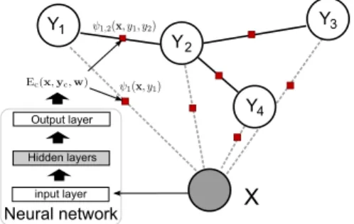
Neural conditional random fields is a combination of NNs and CRFs. They extend CRFs by placing a NN structure between input and energy function. This NN, visualized in Figure 1, is described in detail next.

X Y1 Y2 Y3 input layer Neural network Output layer Hidden layers Y4

Figure 1: Example of a tree-structured NeuroCRF The NN takes an observation as input and outputs a number of quantities which we call energy outputs2 {Ec(x,yc,w)|c,yc} parameterized by w. The NN is feed forward with multiple hidden layers, non-linear hidden units, and an output layer with linear output units (i.e. a linear activation function). With this setting, a NeuroCRF may be viewed as a standard log-linear CRF working on the high-level representation computed by a neural net. In the remainder of the paper we call the top part (output layer weights) of a NeuroCRF its CRF-part and we call the remaining part its deep-part (see Figure 2-right). Let w_nn and wyc

c be the neural net weights of the deep-part and

2

We use the terminology energy output to stress the difference between NN outputs and model outputsy.

the CRF-part respectively. NeuroCRF implements the conditional probability as:

p(y|x)∝Y

c∈C

e−Ec(x,yc,w)₌ Y c∈C

ehwycc,Φc(x,wnn)i ₍₃₎

where Φc(x,wnn) stands for the high level

representa-tion of the input xat clique c computed by the deep part. This is illustrated in Figure 2-left, where the last hidden layer includes units that are grouped in a num-ber of sets, e.g. one for every clique Φc(x,w_nn). Each output unit−Ec(x,yc,wc) is connected to Φc(x,wnn)

in the last hidden layer, with the weight vector wyc

c . Note that the number of energy outputs for each clique cequals|Yc|, hence there are|Yc|weight vectorswyc

c for each clique c.

Inference in NeuroCRFs consists of finding_bythat best matches inputx(i.e. with lowest energy):

b

y = argmax_yp(y|x,w) = argmin_yP

c∈CEc(x,yc,w)

(4)

This can be done in two steps. First one feeds the NN with input x and forward information to compute all energy outputs Ec(x,yc,w). In a second step one uses dynamic programming to find the output _by with the lowest energy.

input layer input layer high-level features

}

}CRF-part deep-part

Figure 2: NN architecture with non shared weights (left) or shared weights (right).

Shared weights network architecture. Various architectures may be used for the NN. One can use a different NN for every energy function, which may result in overfitting and high computational cost. In-stead, as we presented NeuroCRFs above, one may share weights to compute a high level representa-tion per clique (and the corresponding energy out-puts) (Figure 2-left). Or one may choose to com-pute a shared high level representation of the input, from which all energy outputs are computed (Figure 2-right). In this latter case a NeuroCRF implements the conditional probability as:

p(y|x)∝Y

c∈C

ehwycc,Φ(x,wnn)i ₍₅₎

2.3 LINEAR CHAIN NEUROCRFS FOR SEQUENCE LABELING

While the NeuroCRF framework we propose is quite general, in our experiments we focused on linear chain

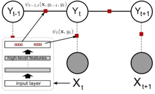
NeuroCRFs based on a first-order Markov chain struc-ture (Figure 3). This allows investigating the potential power of NeuroCRFs on standard sequence labeling tasks. In a chain-structured NeuroCRF there are two kinds of cliques:

• local cliques (x, yt) at each position t, whose po-tential functions are noted by ψt(x, yt), and cor-responding energy functions are noted by Eloc

• transition cliques(x, yt−1, yt) between two succes-sive positions att−1 andt, whose potential func-tions are noted as ψt−1,t(x, yt−1, yt), and corre-sponding energy functions are noted by Etra

Y_t-1 Y_t

X

X

X

Figure 3: A chain-structured NeuroCRF In such models it is usual to consider that energy func-tions are shared between similar cliques at different times (i.e. positions in the graph) (Lafferty, 2001)3_. Then energy functions take an additional argument to specify the position in the graph, which is timet.

ψt(x, yt) =e−Eloc(x,t,yt,w) ψt−1,t(x, yt−1, yt) =e−Etra(x,t,yt−1,yt,w)

(6)

The additional parametertallows the consideration of a part of inputx, whose size may vary and cannot be handled by a fixed size input NN. Time is used to build the input to the NN in order to compute Eloc(x,t,yt). It may consist of xt, the tth element of x only (see Figure 3), or it may include a richer temporal context such as (xt−1, xt, xt+1). At the end, the conditional probability of output ygiven inputxis defined as:

p(y|x,w) =e− P t≥1 Eloc (x,t,yt,w)− P t>1 Etra (x,t,yt−1,yt,w) Z(x) (7) with Z(x) being the normalization factor. With this modeling, one can derive a compact architecture of a NN with |L|+|L|2 _{outputs to compute all energy} outputs.

3

These authors consider two set of parameters, one for local cliques and one for transition cliques.

3

PARAMETER ESTIMATION

Let (x1,y1), ...,(xn,yn)∈ X × Y be a training set ofn

input-output pairs. We seek parameters wsuch that:

yi= argmax

y∈Y

p(y|xi,w) (8)

This translates into a general optimization problem: min

w λΩ(w) +R(w) (9)

where R(w) = _n1P

iRi(w) is a data-fitting measure-ment (e.g. empirical risk), and Ω(w) is a regularization term, withλbeing a regularization factor that is used to find a tradeoff between a good fit on training data and a good generalization. A common choice of Ω(w) is to use L2regularization.

Now, we discuss different criterion for training Neuro-CRFs. Then, we explain how we optimize these cri-terion to learn NeuroCRFs. Finally, we discuss about regularization and evoke semi-supervised learning.

3.1 CRITERIA

There are many discriminative criteria for training CRFs (more generally log-linear models), which can all be used for learning NeuroCRFs as well.

Probabilistic criterion. In (Lafferty, 2001), esti-mation of CRF parameterswwas done by maximizing the conditional likelihood (CML) which results in:

RCM L_i (w) =−logp(yi|xi,w) =P cEc(xi,yic,w) +P y∈Yexp[− P cEc(xi,yc,w)] (10)

Large margin criterion. The large margin method focuses more directly on giving highest discriminant score to the correct output. In NeuroCRFs, the dis-criminant function is a sum of energy functions over cliques (see Eq. (4)):

F(x,y,w) =−X

c∈C

Ec(x,yc,w) (11)

Large margin training for structured output (Taskar et al., 2004) aims at findingw so that:

F(xi,yi,w)≥F(xi,y,w) + ∆(yi,y)∀y∈ Y (12) where ∆(yi_{,y) allows taking into account differences} between labelings (e.g. Hamming distance between y

and yi). We assume a decomposable loss (alike Ham-ming distance) such that ∆(yi,y) = P

cδ(y i c, yc) so that it can be factorized along the graph structure and

integrated in the dynamic programming pass needed to compute argmaxy∈Yp(y|x).

The elementary loss function of NeuroCRFs is then:

RLM i (w)

= maxy∈YF(xi,y,w)−F(xi,yi,w) + ∆(yi,y) = maxy∈YPc∆Ec(xi,yci,yc,w) +δ(yic,yc)

(13) with ∆Ec(xi,yci,yc,w) = Ec(xi,yic,w)−Ec(xi,yc,w). Perceptron approach. Perceptron learning is a simple approach for discriminative training which has been originally proposed for training linear classifiers (Rosenblatt, 1988) but can also be applied to graphi-cal models (Collins, 2002). The idea can be extended to NeuroCRFs by considering the following loss term:

RP erc_i (w) = max y∈Y X c Ec(xi,yic,w)− X c Ec(xi,yc,w) (14) which is very similar to the large margin criterion.

3.2 LEARNING

Due to non-convexity, initialization is a crucial step for NN learning, especially in the case of deep archi-tectures (see (Erhan et al., 2009) for an analysis). For-tunately, an unsupervised greedy-wise pretraining al-gorithm for deep architectures has recently been pro-posed to tackle this problem with notable success (Hin-ton et al., 2006). (Bengio et al., 2006) provides a com-prehensible analysis about greedy pretraining. We de-scribe in detail NN initialization first, then we discuss fine tuning the NeuroCRF.

3.2.1 INITIALIZATION

Initialization of hidden layers in the NeuroCRF is done incrementally as it has been popularized for learning deep architectures. In our implementation, the deep-part of the NeuroCRF is initialized layer by layer in an unsupervised manner using restricted Boltzmann ma-chines4(RBMs) as proposed by Hinton and colleagues (Hinton et al., 2006). Depending on the task, inputs may be real valued or binary valued, this may be han-dled by slightly different RBMs. We considered both cases in our experiments, while coding (hidden) layers always consisting of binary units.

Once a cascade of successive RBMs have been trained one at a time, one obtains a deep belief net which is then transformed into a feed forward NN which imple-ments the deep-part of the NeuroCRF (without out-put layer). Once the deep-part is initialized, the NN is

4

The NN weights are initialized with zero-mean Gaus-sian noise before RBM learning.

used to compute a high-level representation (i.e. the vector of activations on the last hidden-layer) of input samples. The CRF-part may then be initialized by training (in a supervised way) a linear CRF with this high-level coding of input samples. As we said, such a linear CRF is actually an output layer which is stacked over the deep part. The union of the weights of the deep-part and of the CRF-part constitutes an

initial-ization solution w0 which is fine tuned, as described

below, using supervised learning.

3.2.2 FINE TUNING

Fine tuning aims at learning the NeuroCRF parame-ters globally based on an initial and reasonable solu-tion. None of the criterion we discussed earlier (Sub-section 3.1) are convex since we naturally consider NNs with non linear (sigmoid) activation functions in hid-den layers. However, provided one can compute an ini-tial and reasonable solution and provided one can com-pute the gradient of the criterion with respect to NN weights, one can use any gradient-based optimization method such as stochastic gradient or bundle method to learn the model and reach a (eventually local) mini-mum. We show now how to compute the gradient with respect to the NN weights.

As long as Ri(w) is continuous and there is an

effi-cient method for computing ∂Ri(w)

∂Ec(x,yc,w) (this is true

for all criteria discussed in the previous section) the

(sub)gradient ofR(w) with respect tow can be

com-puted with a standard backpropagation procedure.

Let Ei be the set of energy outputs corresponding to

inputxi_{. Using the chain rule for every} ∂Ri(w)

∂w : ∂R(w) ∂w = 1 n X i ∂Ri(w) ∂w = 1 n X i ∂Ri(w) ∂Ei ∂Ei ∂w (15)

where ∂_∂Ei_w is the Jacobian matrix of the NN outputs

(for inputxi) with respect to weightsw. Then by setting ∂R_∂i(w)_E

i as backpropagation errors of

the NN output units, we can backpropagate and get ∂Ri(w)

∂w using the chain rule over hidden layers.

3.2.3 REGULARIZATION AND

SEMI-SUPERVISED LEARNING

In our implementation, we used the initial solution for building a quadratic regularization term of the form:

Ω(w) = 1

2kw−w0k

2 ₍₁₆₎

The idea is that since the deep-part of a NeuroCRF is initialized in an unsupervised manner, we may expect using this solution for regularizing will avoid overfit-ting during fine tuning (we found that this gives better

experimental results than using standard regulariza-tion by 0). Since the CRF-part is not initialized with a generative model, we regularize this part with 0 -both for initialization and fine-tuning.

Note that NeuroCRF permits semi-supervised learn-ing in a very natural way. Indeed one may easily use unlabeled data for initializing the deep-part while la-beled data are used in fine tuning only. One can ex-pect that a good initialization of the deep-part will improve the global performance of a NeuroCRF, since the deep-part plays an important role of finding a rel-evant high-level representation of the input. It is a perspective of our work that we did not explore yet.

4

EXPERIMENTS

We performed experiments on two sequence labeling tasks with two well-known datasets. We first investi-gate the behaviour of NeuroCRFs in a first series of ex-periments on Optical Character Recognition with the OCR dataset (Kassel, 1995). Then we report exper-imental comparative results of NeuroCRFs and state of the art methods for the more complex task of au-tomatic speech recognition using the TIMIT dataset (Lamel et al., 1986). In both cases we replicated ex-perimental settings of previous works in order to get fair comparison, building on the compilation of Ben

Taskar5for the OCR dataset, and using standard

par-titioning of the data and standard preprocessing for the TIMIT corpus. We use linear chain NeuroCRF for both tasks.

In fine-tuning we use a variant of our batch optimizer named non-convex regularized bundle method (Do &

Arti`eres, 2009) rather than a stochastic gradient

pro-cedure. As usual in bundle methods, our stopping con-dition is based on the Gap (G) between the Best ob-served objective function value (B) and the minimum of the approximation. We stop when the ratio of G/B is below 1%. This is a good trade-off for reaching low error-rates with a limited number of iterations (100 for OCR, 150 for ASR experiments).

4.1 OPTICAL CHARACTER RECOGNITION

OCR dataset consists of 6877 words which correspond to roughly 52K characters (Kassel, 1995; Taskar et al., 2004). OCR data are sequences of isolated characters (each represented as a binary vector of dimension 128) belonging to 26 classes. The dataset is divided in 10 folds for cross validation. We investigated two settings, using a large training set by training on 9 folds and testing on 1 fold (this is thelarge setting) and using a

5

small one by training on 1 fold and testing on 9 folds

(this is the small setting). Note that OCR results

are cross-validation results, we do not use any extra validation set to set lambda.

We learned NeuroCRFs with one or two hidden layers. Transition energy outputs has only one connection to a bias unit, meaning that we do not use any input in-formation for building transition energy. We learned standard RBMs for initializing the deep part of Neu-roCRFs, which are learned with 50 iterations through the training set. Learning is performed using 1 step Contrastive Divergence.

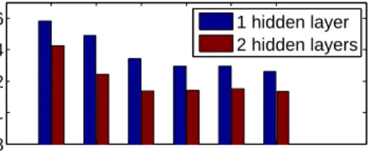
Influence of network architecture. Figure 4

re-ports error rates gained on thesmallsetting with

Neu-roCRF with one or two hidden layers of varying size. As can be seen, increasing the size of hidden layers

im-50 100 200 300 400 500 0.08 0.1 0.12 0.14 0.16

number of hidden units per layer

error rate

1 hidden layer 2 hidden layers

Figure 4: Influence of NN architecture on OCR dataset (small training set).

proves performance for one hidden layer and two hid-den layer NeuroCRFs. Also two hidhid-den layers architec-tures systematically outperform single hidden layer ar-chitectures. Note that whatever the number of hidden layers, performance reaches a plateau when increasing the hidden layers’ size. However the plateau is lower and reached faster for the two hidden layer architec-ture. These results suggest that increasing both the size of hidden layers and the number of hidden layers may significantly improve performance.

Accuracy. We compared the performance of two variants of NeuroCRFs, one trained with conditional maximum likelihood (CML), the other one trained with a large margin criterion (LM) with state of the art methods : linear and cubic M3Ns, linear CRFs, con-ditional neural fields (CNFs) with one hidden layer. NeuroCRFs have 2 hidden layers of 200 units each. Table 1 reports cross validation error rates of these

models for thesmall setting and thelargesetting. We

also report the performance of initial solutions (i.e. before fine tuning) for NeuroCRFs (in brackets). NeuroCRFs significantly outperform all other meth-ods, including M3N with non-linear kernel (whose

re-Table 1: Comparative error rates of NeuroCRF and state of the art methods on OCR dataset with either a small and a large training sets. Performance of Neuro-CRF before fine tuning are indicated in brackets. Re-sults of SVM cubic, M3N cubic and CNF come from (Taskar et al., 2004; Peng et al., 2009).

small large

CRF linear 0.2162 0.1420

M3N linear 0.2113 0.1346

SVM cubic 0.19 not available

M3N cubic 0.13 not available

CNF 0.131 not available

NeuroCRFCM L _{0.1080(0.1224) 0.0444(0.0697)}

NeuroCRFLM _{0.1102(0.1221) 0.0456(0.0736)}

sults are not reported for the large setting due to scala-bility). Also looking at the performance of NeuroCRF before fine tuning shows that initialization by RBMs and CRFs indeed produce a good starting point, but fine tuning is essential for obtaining optimal perfor-mance. Finally, one sees here that both NeuroCRF training criteria are similar with a slight advantage of conditional likelihood criterion on large margin crite-rion. Surprisingly, we observed that the large margin criterion required more iterations than the conditional likelihood criterion6. In the following, we only consid-ered NeuroCRFs trained with the CML criterion. Note that (Perez-Cruz & Pontil, 2007) address the structured prediction with a different way and they are able to reach an error rate of 0.125 in small setting and 0.031 in large setting (using RBF kernel). Their approach considers an approximated problem that can be transformed into many multiclass SVM problems. Nevertheless, the non-linear SVM problems still scale quadratically with the problem size. Such a scaling prevents working with large data sets with millions of tokens (such as ASR experiments in next section).

Training time. We investigated the learning time of NeuroCRF and its scalability. We performed

ex-periments on the OCR dataset both for small and

large settings. Training time decomposes into RBM unsupervised learning, linear CRF initialization, and fine tuning the whole model. Roughly speaking RBM learning and fine tuning take about 45% of the time each, while CRF initialization takes about 10%. More

importantly, overall training time in the large setting

took about 10 times the training time in thesmall

set-ting while the training dataset is 9 times bigger, which 6

Actually we did not succeed at optimizing the large margin criterion. We conjecture that the parameter search space might be more complex in this case.

suggests a quasi-linear scaling with the problem size.

4.2 AUTOMATIC SPEECH

RECOGNITION

We performed ASR experiments on the TIMIT dataset (Lamel et al., 1986) with standard train-test partition-ing. The wave signal was preprocessed using the pro-cedure described in (Sha & Saul, 2007), except that we do not use whitening by PCA. The 39-dimensional MFCC are simply normalized to have zero mean and unit variance. There are roughly 1.1 million frames in the training set, 120K frames and 57K frames re-spectively in the development and test sets. We used 2-layered NeuroCRFs trained with the CML criterion. Handling continuous feature. Note here that in-puts (real valued vectors of MFCC coefficients) are continuous while RBMs originally use binary logistic units for both visible and hidden variables. We used an extension of RBM for dealing with continuous vari-ables that have Gaussian noise (In our implementation we consider a Gaussian noise with standard derivation 0.2) (Taylor et al., 2007). ThisGaussian-BinaryRBM was trained for 100 passes through the training data of 1.1M frames, using one step Contrastive Divergence. Once this first RBM is trained, we forward the input to the hidden layer and obtain a binary-logistic repre-sentation of the speech data, which is the inputs (i.e. visible data) for learning a second binary RBM. Since binary RBM converge much faster, we performed only 10 learning iterations through the training data for the second layer. The remaining initialization is performed as in section 3.2.1.

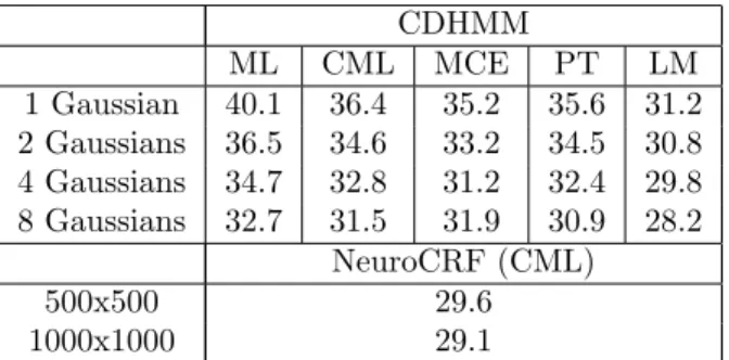
Table 2: Comparative phone recognition error rate on TIMIT dataset for discriminant and non discriminant HMM systems and for two hidden layer NeuroCRFs (of 500 or 1000 hidden units each) trained with CML.

CDHMM ML CML MCE PT LM 1 Gaussian 40.1 36.4 35.2 35.6 31.2 2 Gaussians 36.5 34.6 33.2 34.5 30.8 4 Gaussians 34.7 32.8 31.2 32.4 29.8 8 Gaussians 32.7 31.5 31.9 30.9 28.2 NeuroCRF (CML) 500x500 29.6 1000x1000 29.1

Results. Table 2 reports the phone error rates for CDHMMs and NeuroCRFs with increasing complex-ity (number of Gaussians in CDHMMs or number of hidden units in NeuroCRFs). We compared

Neuro-CRFs with non discriminant CDHMMs (i.e.

Maxi-mum Likelihood) and with state of the art approaches for learning CDHMMs with a discriminant criterion, Maximum Conditional Likelihood (CML) (Woodland & Povey, 2002), Minimum Classification Error (MCE) (Juang & Katagiri, 1992), Large margin (LM) (Sha & Saul, 2007), Perceptron learning (PT) (Cheng et al., 2009) (note that all results come from a compilation in (Sha & Saul, 2007) and from (Cheng et al., 2009)). These results call for a few comments. First increasing the hidden layers’ size improves the NeuroCRF error rate. Unfortunately we do not know if it still improves when using larger hidden layers (due to lack of time) but one can reasonably expect that even better results may be reached by using larger hidden layers and/or adding hidden layers. Second, NeuroCRFs outperform all other discriminant and non discriminant methods except Large Margin training of (Sha & Saul, 2007) when using up to 8 Gaussian distributions per state. While this may not look like an impressive result at first glance, we claim this result to be very promis-ing. Indeed, all other systems in Table 2 rely on the learning of a preliminary CDHMM system, which is then used as initialization and/or for regularization. Hence all these systems integrate prior information from decades of research on how to learn and tune a non discriminant CDHMM for speech. In contrast NeuroCRF are trained from scratch with a non super-vised initialization and a supersuper-vised fine tuning, they require no prior information.

Note that we did not compare NeuroCRF to multiple states per phone CDHMM systems as those tradition-ally used in ASR although such systems may reach bet-ter performance (especially for ML CDHMM). Reason is that comparison would have not been so fair. Indeed one may imagine extending this work in order to have multiple nodes per phone in NeuroCRF and one may expect this to provide even better results, that would be more directly comparable with multiples states per phone HMM systems.

5

CONCLUSION

We presented a model combining CRFs and deep NNs aiming at taking advantage of both the ability of deep networks to extract high level features and the dis-criminant power of CRFs for sequence labeling tasks. Results on OCR data show significant improvement over state of the art methods and demonstrate the rel-evance of the combination. On the larger scale speech recognition task our systems outperform most state of the art discriminant systems without relying on any prior in contrast to all other systems relying on an ini-tial solution gained with a non discriminant criterion.

Acknowledgements

Authors acknowledge the support by PASCAL 2 EU Network of Excellence.

References

Altun, Y., Johnson, M., & Hofmann, T. (2003). Inves-tigating loss functions and optimization methods for discriminative learning of label sequences. EMNLP. Bengio, Y., Lamblin, P., Popovici, D., & Larochelle, H. (2006). Greedy layer-wise training of deep networks

(Technical Report 1282). Universit´e de Montr´eal. Bengio, Y., & LeCun, Y. (2007). Scaling learning

algo-rithms towards ai. In Large scale kernel machines. Cambridge, MA: MIT Press.

Bottou, L., Bengio, Y., & LeCun, Y. (1997). Global training of document processing systems using graph transformer networks. In Proc. of Com-puter Vision and Pattern Recognition(pp. 490–494). Puerto-Rico. IEEE.

Cheng, C.-C., Sha, F., & Saul, L. K. (2009). Matrix updates for perceptron training of continuous den-sity hidden markov models. ICML(pp. 153–160). Collins, M. (2002). Discriminative training methods

for hidden markov models: theory and experiments with perceptron algorithms. EMNLP (pp. 1–8). Collobert, R., Sinz, F., Weston, J., & Bottou, L.

(2006). Trading convexity for scalability. ICML. Do, T.-M.-T., & Arti`eres, T. (2009). Large margin

training for hidden Markov models with partially observed states. ICML(pp. 265–272). Omnipress. Erhan, D., Manzagol, P.-A., Bengio, Y., Bengio, S.,

& Vincent, P. (2009). The difficulty of training deep architectures and the effect of unsupervised pre-training. AISTATS.

Graves, A., Fern´andez, S., Gomez, F., & Schmidhuber, J. (2006). Connectionist temporal classification: la-belling unsegmented sequence data with recurrent neural networks. ICML(pp. 369–376).

Hinton, G. E., Osindero, S., & Teh, Y.-W. (2006). A fast learning algorithm for deep belief nets. Neural Computation,18, 1527–1554.

Juang, B., & Katagiri, S. (1992). Discriminative learn-ing for minimum error classification. IEEE Trans. Signal Processing, Vol.40, No.12.

Kassel, R. H. (1995). A comparison of approaches to on-line handwritten character recognition. Doctoral dissertation, Cambridge, MA, USA.

Lafferty, J. (2001). Conditional random fields: Proba-bilistic models for segmenting and labeling sequence data. ICML(pp. 282–289). Morgan Kaufmann. Lafferty, J., Zhu, X., & Liu, Y. (2004). Kernel

condi-tional random fields: representation and clique se-lection. ICML.

Lamel, L., Kassel, R., & Seneff, S. (1986). Speech database development: Design and analysis of the acoustic-phonetic corpus. DARPA(pp. 100–110). LeCun, Y., Bottou, L., Bengio, Y., & Haffner, P.

(1998). Gradient-based learning applied to docu-ment recognition. Proceedings of the IEEE,86. Mccallum, A., Freitag, D., & Pereira, F. (2000).

Max-imum entropy markov models for information ex-traction and segmentation. ICML(pp. 591–598). Peng, J., Bo, L., & Xu, J. (2009). Conditional neural

fields. NIPS.

Perez-Cruz, F, G. Z., & Pontil, M. (2007). Condi-tional graphical models. In G. H. Bakir, T. Hof-mann, B. Schlkopf, A. J. Smola, B. Taskar and S. V. N. Vishwanathan (Eds.),Predicting structured data. MIT Press.

Qi, Y., Kuksa, P. P., Collobert, R., Sadamasa, K., Kavukcuoglu, K., & Weston, J. (2009). Semi-supervised sequence labeling with self-learned fea-tures. ICDM’09. IEEE.

Rosenblatt, F. (1988). The perceptron: a probabilistic model for information storage and organization in the brain.Neurocomputing: foundations of research, 89–114.

Sato, K., & Sakakibara, Y. (2005). Rna secondary structural alignment with conditional random fields.

ECCB/JBI(p. 242).

Sha, F., & Saul, L. K. (2007). Large margin hid-den markov models for automatic speech recogni-tion. NIPS 19(pp. 1249–1256). MIT Press. Taskar, B., Guestrin, C., & Koller, D. (2004).

Max-margin markov networks. NIPS 16. MIT Press. Taylor, G. W., Hinton, G. E., & Roweis, S. T. (2007).

Modeling human motion using binary latent vari-ables. InNips, 1345–1352. MIT Press.

Woodland, P., & Povey, D. (2002). Large scale dis-criminative training of hidden markov models for speech recognition.Computer Speech and Language,