Modeling spatial covariance functions

Open Access Dissertations Theses and Dissertations

Summer 2014

Modeling spatial covariance functions

InKyung Choi

Purdue University

Follow this and additional works at:https://docs.lib.purdue.edu/open_access_dissertations

Part of theApplied Statistics Commons

This document has been made available through Purdue e-Pubs, a service of the Purdue University Libraries. Please contact [email protected] for additional information.

Recommended Citation

Choi, InKyung, "Modeling spatial covariance functions" (2014).Open Access Dissertations. 246.

PURDUE UNIVERSITY

GRADUATE SCHOOL

Thesis/Dissertation Acceptance

+HDGRIWKHDepartment *UDGXDWH3URJUDP 'DWH

To the best of my knowledge and as understood by the student in the Thesis/Dissertation Agreement, Publication Delay, and Certification/Disclaimer (Graduate School Form 32), this thesis/dissertation adheres to the provisions of Purdue University’s “Policy on Integrity in Research” and the use of copyrighted material.

InKyung Choi

MODELING SPATIAL COVARIANCE FUNCTIONS

Doctor of Philosophy Hao Zhang Bo Li Xiao Wang Tonglin Zhang Hao Zhang Rebecca W. Doerge 08/29/2014

A Dissertation Submitted to the Faculty

of

Purdue University by

InKyung Choi

In Partial Fulfillment of the Requirements for the Degree

of

Doctor of Philosophy

December 2014 Purdue University West Lafayette, Indiana

ACKNOWLEDGMENTS

First of all, I want to express my sincere gratitude to my advisor Professor Hao Zhang. He encouraged independent thinking and supported my ideas, which allowed me to freely pursue and explore topics that interested me, and whenever I went astray, his insightful comments put me back on the right track.

I am also greatly indebted to Professor Bo Li who had been my advisor for the first three years of the Ph.D. program. I cannot overstate her influence at the beginning of my research in the field of Spatial Statistics. Her extensive knowledge about the field and passion for research had been an inspiration to me. Even after moving to the University of Illinois at Urbana-Champaign, she has always taken good care of me and put herself out of the way to support me.

I appreciate my committee members; Professor Xiao Wang and Professor Tonglin Zhang for their helpful input and warm encouragement. The support of the Depart-ment of Statistics and the staff members should not go unDepart-mentioned for it was only through their consistent help and assistance that I could complete my study.

I was fortunate to study at university that hosts a great consulting center like Statistical Consulting Service center. While working at the center, I learnt a great deal about how to apply statistics in practice, knowledge that can not be easily obtained in a classroom. The invaluable experience that I had obtained through working with clients from various fields will be of a great asset for the rest of my professional career and I am thankful for all the professors, colleagues and staff members of the center, and especially Professor Bruce Craig for his guidance and mentoring.

In a seemingly endless fight with oneself and facing the battle all alone in a foreign country, I often found facets of myself that I had never truly realized before. Hence the last five years has not only been about the pursuit of academic knowledge but also a journey to understand myself, and perhaps the world around me as well. My friends

both inside and outside the department have been wonderful companions along the journey and I’m grateful to them for being good friends and teachers during the important time of my life.

Lastly, I want to thank my family in Korea. Although separated by continents, knowing that I have people who always love and support me without condition gave me strength and courage to go on even in the darkest night. I’m forever indebted for their unwavering devotion which is the true force that has shaped who I am now.

TABLE OF CONTENTS

Page

LIST OF TABLES . . . vi

LIST OF FIGURES . . . vii

ABSTRACT . . . viii

1 INTRODUCTION . . . 1

1.1 Motivation . . . 1

1.2 Preliminaries . . . 2

1.2.1 Covariance function of random fields . . . 2

1.2.2 Spectral representation of stationary covariance functions . . 4

1.2.3 Some nonstationary covariance functions . . . 5

1.2.4 Spatial random effect model . . . 6

1.3 Overview. . . 8

2 NONPARAMETRIC COVARIANCE ESTIMATION . . . 9

2.1 Introduction . . . 9

2.2 Nonparametric Covariance Estimation . . . 12

2.2.1 Construction of completely monotone function . . . 12

2.2.2 Estimation. . . 14

2.3 Extension to Space-Time Covariance Function . . . 17

2.4 Simulation Study . . . 19

2.4.1 Simulation set up . . . 20

2.4.2 Number of knots and order of B-splines . . . 21

2.4.3 Comparison with parametric models . . . 22

2.4.4 Simulation with space-time covariance function . . . 25

2.5 Two Data Examples . . . 27

2.5.1 Indiana July mean temperature data . . . 27

2.5.2 Irish wind data . . . 29

2.6 Conclusion . . . 33

3 ANALYSIS OF TELECONNECTION . . . 35

3.1 Introduction . . . 35

3.2 ENSO Teleconnection to North America . . . 38

3.3 Model for Time-varying Teleconnection . . . 42

3.3.1 Model . . . 43

Page 3.3.3 Empirical confidence interval for covariance of spatial random

effect . . . 48 3.4 Data Analysis . . . 50 3.4.1 Teleconnection analysis . . . 50 3.4.2 Spatial prediction . . . 57 3.5 Conclusion . . . 63 REFERENCES . . . 65 VITA . . . 70

LIST OF TABLES

Table Page

2.1 Mean and standard error (in parenthesis) of integrated squared error (ISE) and mean squared prediction error (MSPE) of nonparametric model at different knot number m and order of B-splines p (unit: 10−2_{). . . . . 23}

2.2 Mean and standard error (in parenthesis) of integrated squared error (ISE) and mean squared prediction error (MSPE) of three parametric models (spherical, Mat´ern and Gaussian) and the nonparametric model (with or-der of B-splines p= 3 and knot number m= 5), together with the MSPE of true covariance model (unit: 10−2_{). . . . . 24}

2.3 Mean and standard error (in parenthesis) of integrated squared error (ISE) and mean squared prediction error (MSPE) of the nonparametric space-time covariance model at different knot number (mφ_{, m}ψ_{) and order of}

B-splines (pφ, pψ) and of the parametric models (unit: 10−2). . . 26 2.4 Mean squared prediction error (MSPE) of one-day ahead prediction of

Irish wind data. . . 32 3.1 Mean of mean squared prediction error (MSPE) and logarithm score (LogS)

of prediction based 1) Two regions : uses both North America data and Ni˜no3 region data; and 2) One region : uses data from the same region as the region of the dropped-site . . . 63

LIST OF FIGURES

Figure Page

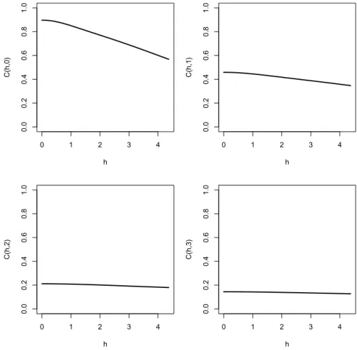
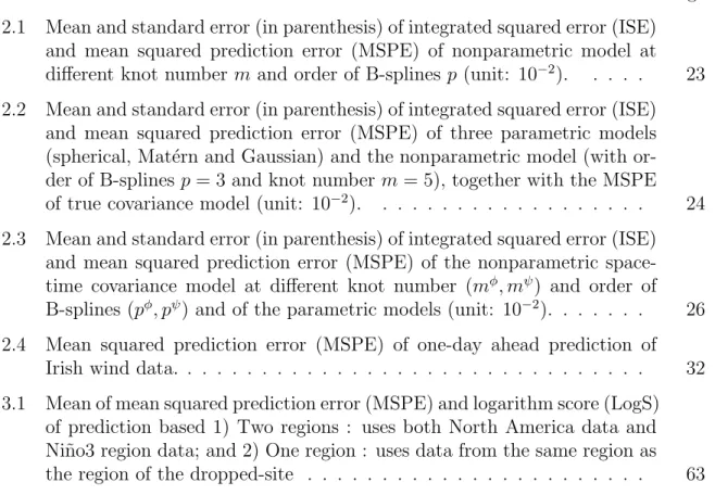
2.1 Example of functions {f_j[q]: j = 1, . . . , m+p} for m = 2 and p = 3, and two covariance functions constructed based on those f_j[q]: C1(h) =

5f₁[2](h2) + 0.5f₅[2](h2) andC2(h) = 0.7f [2]

3 (h2) + 0.1f [2]

4 (h2). . . 15

2.2 86 weather stations in Indiana with July 2011 mean temperatures, together with temperature surface interpolated using the fitted nonparametric co-variance function . . . 28

2.3 Emprical covariance estimates (dots) and fitted covariance functions for Indiana July 2011 temperature data (distance unit: 10 km) . . . 29

2.4 Empirical covariance estimates (dots) of Irish wind data and fitted non-parametric model (solid line) at four different sets of space-time lags (dis-tance unit: 100 km) . . . 31

3.1 Nino3 region and North America region . . . 41

3.2 Temporal variation of residual variance (top: Ni˜no3 region; bottom: North America) before standardization (blue lines) and after the standardization (red lines) . . . 51

3.3 Location of centers of spatial basis functions . . . 52

3.4 Estimated covariances ˆσij(t) from 1871 to 1990 . . . 53

3.5 Estimated covariances ˆσij(t) from 1871 to 1990 . . . 54

3.6 Estimated covariance σ_bij(t) for spatial random effectsα1, . . . , α6 . . . . 55

3.7 Estimated covariance σ_bij(t) for spatial random effectsα7, . . . , α12 . . . 56

3.8 Mean and empirical confidence interval of covariances associated with α1, . . . , α4 . . . 58

3.9 Mean and empirical confidence interval of covariances associated with α6, α7, α8 and α10 . . . 59

3.10 Squared Frobenius norm of estimated cross-region covariance matrix. . 60 3.11 Location of centers of spatial basis functions for spatial prediction; 20 (14)

new basis functions are added to 12 (6) basis functions of North America (Ni˜no3 region) used in teleconnection analysis (rA = 32 and rB = 20) . 61

ABSTRACT

Choi, InKyung Ph.D., Purdue University, December 2014. Modeling spatial covari-ance functions. Major Professor: Hao Zhang.

Covariance modeling plays a key role in the spatial data analysis as it provides important information about the dependence structure of underlying processes and determines performance of spatial prediction. Various parametric models have been developed to accommodate the idiosyncratic features of a given dataset. However, the parametric models may impose unjustified restrictions to the covariance structure and the procedure of choosing a specific model is often ad-hoc. In the first part of the dissertation, a new nonparametric covariance model that can avoid the choice of parametric forms is proposed. The estimator is obtained via a nonparametric approx-imation of completely monotone functions. It is easy to implement and simulation study shows it outperforms the parametric models when there is no clear information on model specification. Two real datasets are analyzed to illustrate the proposed approach and provide further comparison between the nonparametric and parametric models.

Most spatial covariance models assume that the dependence becomes stronger when two locations are closer to each other and thus assume that the dependence is negligible when two locations are far apart from one another. However long-distance connection can occur in climate variables through, for example, high altitude winds or large-scale atmospheric waves propagation. This phenomenon is called teleconnection and often considered to be responsible for extreme weather events occurring simul-taneously around the world. In the second part of the dissertation, a nonstationary spatial covariance model for long-distance dependence is proposed. The model allows the spatial dependence to vary with time so that temporal dynamics of the

telecon-nection phenomenon can be captured. The model is applied to analyze telecontelecon-nection between sea surface temperature of tropical Pacific Ocean and hydrological droughts of North America incurred by the El Ni˜no-Southern Oscillation.

1. INTRODUCTION

1.1 Motivation

As time series data are often assumed to be a realization of a stochastic process defined on an ordered set, a random field has been a primary mathematical framework of choice for analysis of spatial data. While time series data are observed at a sequence on one dimension of time, spatial data are observed over a two-dimensional plane or even in a higher dimensional space. This complicates the problem of dependence modeling because we now have another aspect to consider: direction of the spatial lag.

One may assume that the dependence strength depends only on the spatial lag length as in time series data analysis and this works reasonably well for many cases where the process can be assumed to be relatively homogeneous across the space. On the other hand, if the spatial domain of interest is over a vast region or has complex geographical features, the assumption may not hold and the dependence may vary by the direction of spatial lag as well as location at which the lag is measured. Indeed, the direction or the location with strong spatial dependence could provide important features of the underlying physical process such as in teleconnection phenomenon (see Chapter 2 for more details).

Once data are observed, they are considered as a realization of a multivariate distribution whose distributional characteristics are inherited from the corresponding random field. Although there are several multivariate dependence concepts (e.g. copula, tail dependence, orthant dependence and etc.), covariance is the most popular measure to quantify spatial dependence in the data for several reasons: the concept is straightforward; it is easy to calculate sample covariances and its properties are well understood. Above all, the best linear spatial predictor (kriging) is expressed

as a function of covariances. Therefore, it is not surprising to find that covariance function modeling plays an important role in spatial data analysis and a lot of effort has been made to develop covariance functions that can accommodate idiosyncratic features of a given dataset.

In the remaining part of this chapter, we give an introduction to basic concepts and background, and provide a brief review of some existing spatial covariance models.

1.2 Preliminaries

1.2.1 Covariance function of random fields

Consider a Gaussian random field {Y(s) : s∈ D⊂ _Rd_{} where D is a domain of}

interest in d-dimensional Euclidean space _Rd_{. A common framework of spatial data}

analysis decomposes the random field into three components (Cressie, 1993):

Y(s) =µ(s) +Z(s) +(s), (1.1)

whereµ(s) is a large-scale variation,Z(s) is a small-scale spatial variation and(s) is a measurement error. The deterministic large-scale variation µ(s) is used to remove the non-stationary component inY(s) that is caused by the varying mean and often takes a form ofµ(s) =x(s)0β_µ, wherex(s) = (x1(s), . . . , xp(s))0 is a vector of known

covariates and β_µ is an unknown parameter vector. The measurement error (s) is assumed to be a zero-mean white noise process with variance Var((s)) = σ2

. The

spatial dependence of Y(s) arises from the dependence within the small-scale spatial variation Z(s) and we focus on modeling the dependence of this process.

Let C :D×D →_R denote the covariance function of random field Z(s):

C(s,u) = Cov(Z(s), Z(u)) s,u∈D. (1.2)

If the mean of the random field is constant (i.e. E(Z(s)) ≡ µ) and the covariance depends on the spatial lags−u between two locations only, i.e.,

for some function CSt _:

Rd → R, the random field is called weakly stationary (also called transional invariant or second-order stationary) and its covariance function is called stationary covariance function. Furthermore, if the covariance function does not depend on the direction of the lags−u, but depends on the length ||s−u||only, i.e.,

C(s,u) = CIso(||s−u||),

for some function CIso _:

R+ →R, the process is called isotropic random field and its covariance function is called isotropic covariance function.

Although the isotropy is a rather strong assumption, isotropic covariance function can serve as a building block in constructing non-isotropic (anisotropic) covariance functions or non-stationary covariance functions. For example, a popular class of anisotropic covariance functions is obtained by a linear transformation of the spatial lag vector h using some matrix A (Journel and Huijbregts, 1978):

CSt(s−u) =CIso(||A(s−u)||), (1.3) or, by extension, CSt(s−u) = m X i=1 C_iIso(||Ai(s−u)||).

A similar approach can be taken to construct non-stationary covariance functions from isotropic covariance functions and this will be described in Section 1.2.3.

In the rest of this dissertation, C (without superscript) will be used to denote a covariance function regardless of the type. It will be obvious from the arguments of the function which type of covariance function is referred to in each context.

Now, forCto be a valid covariance function, it needs to satisfy the positive definite condition, i.e., n X i=1 n X j=1 aiajC(si,sj)>0, (1.4)

for any finite set of spatial locations s1, . . . ,sn ∈ D and real numbers a1, . . . , an.

as complete monotonousness (see Section 2.2.1), but the condition can be more easily checked in the spectral domain using spectral representation as described in following Section 1.2.2.

1.2.2 Spectral representation of stationary covariance functions

By spectral representation theorem, a weakly stationary random field Z(s) can be represented in the form of Fourier-Stieltjes integral as:

Z(s) =

Z

Rd

exp(is0ω)dX(ω), (1.5)

whereX(ω) is a zero-mean process with independent increments. SinceX(ω) in (1.5) is an independent process, we can write the covariance function of the random field Z(s) as: C(h) = E Z Rd exp(iω00)dX(ω) Z Rd exp(iω0h)dX(ω) = Z Rd exp(ih0ω)F(dω), (1.6)

whereF(ω) = E[|dX(ω)|2_{] is called the spectral measure whose density with respect}

to Lebesgue measure, if exists, is called the spectral density function. It is straight-forward to show thatC(h) is positive definite if it has representation (1.6) because

n X i=1 n X j=1 aiajC(si−sj) = Z Rd | n X j=1 ajexp(is0jω)| 2 F(dω)≥0.

In fact, every positive definite function has this representation (Bochner’s theo-rem) and (1.6) is the only way to obtain a valid covariance function.

Now, spectral representation (1.6) can be simplified if we further assume that the covariance function is isotropic. Then, for h∈ _R+_{, the isotropic covariance function}

C(h) can be represented as:

C(h) = Z ∂bd C(h||v||)U(dv) = Z ∂bd Z Rd exp(ihv0ω)F(dω)U(dv),

for an uniform probability measureU ond-dimensional unit sphere∂bd(Stein, 1999).

Then, using spherical coordinate system and integrating out the angular variable, we can obtain that

C(h) = Z ∞ 0 Γ(d/2) 2 hω (d−2)/2 J(d−2)/2(hω)dH(ω), (1.7)

whereJν(·) is a Bessel function of the first kind of orderν andH(ω) = R

||ω||<ωF(dω).

Many of commonly used isotropic spatial covariance functions have the representa-tion (1.7). For example, spectral densities of exponential covariance funcrepresenta-tion and gaussian covariance function are proportional to bivariate Cauchy probability density and normal probability density respectively. Mat´ern covariance function has a spec-tral density proportional to student-t density, which explains, in the specspec-tral domain, how exponential and Gaussian covariance functions are the special cases of Mat´ern family. Indeed it is this representation (1.7) of an isotropic covariance function that has contributed to the development of many nonparametric covariance models (see Section 2.1 for more details).

1.2.3 Some nonstationary covariance functions

Stationary covariance functions may work well if one considers a relatively small region or if it is reasonably believed that the process in the region of interest would exhibit homogenous characteristics. But when the spatial domain is vast, it is more realistic to assume that the dependence structure changes over the space. For ex-ample, the same spatial lag h may imply different degree of dependence strength depending on where the lag is measured, i.e.,

C(s,s+h)6=C(u,u+h), s6=u.

As in the construction of anistropic covariance function (1.3), nonstationary co-variance functions can be obtained from isotropic coco-variance functions. “Image wrap-ping” is one of such attempts. Sampson and Guttorp (1992) pioneered the the work on the use of space deformation techniques in developing nonstationary covariance

functions. They extended linear transformation (1.3) to a smooth non-linear trans-formationf :_Rd→_Rd0_:

C(s,u) = CIso(|f(s)−f(u)|),

so that the covariance function is isotropic in a transformed space f(s).

Convolution-based methods have also been employed to create nonstationary co-variance functions. In these approaches, a nonstationary coco-variance function is ob-tained by defining a convolution process instead of specifying a particular form of covariance function. For example, in Higdon, Swall and Kern (1999), a nonstation-ary process is defined as the convolution of some kernel function K and white noise process X(v):

Z(s) =

Z

Rd

K(s−v)X(v)dv, (1.8)

while in Fuentes and Smith (2001), the nonstationary process is defined as: Z(s) =

Z

Rd

K(s−v)Xθ(v)(s)dv, (1.9)

where {Xθ(v)(s) : s,v ∈ Rd} are independent white noise processes indexed by

pa-rameter θ(v). The covariance function can be obtained directly from the definition. For example, from (1.9), we have

C(s,u) =

Z

Rd

K(s−v)K(u−v)Cθ(v)(s−u)dv, (1.10)

which is obviously nonstationary. These types of nonstationary covariance functions are considered as a ‘local’ approach because locally stationary processes are used to create a globally nonstationary process, hence generating a globally nonstationary covariance function.

1.2.4 Spatial random effect model

In recent years, large-scale data are becoming more and more common due to the advancement of high-resolution satellite data and climate product data. Also, existing

historic datasets, such as sea surface temperature measurements from ships or buoys, which are very sparse individually, are combined and interpolated together to pro-duce a high resolution global dataset. These massive datasets incur a computational burden both in estimating the covariance function and making spatial prediction at an unknown location because such procedures often involve inverting an×nvariance matrix, wheren is the size of the dataset. For this reason, the massive dataset prob-lem has gained much attention in the spatial statistical community, and the spatial random effect model is proposed to tackle this problem.

In the spatial random effect model, the small-scale variation Z(s) in the random field Y(s) is described using a set of latent variables (random effects) {αr}r=1,...,R

with spatial basis functions{fr(s)}r=1,...,R:

Y(s) = µ(s) +

R X

r=1

αrfr(s) +(s).

Similar to the random effect model in the experimental design, the dependence among data arises from sharing the latent variables and the degree of communality is ad-justed by weights assigned through spatial basis functions. The covariance function of random fieldY(s) is:

C(s,u) =f0_sKf_u+σ2δ{s=u}, (1.11)

where f_s is a R ×1 vector of spatial basis functions evaluated at spatial location

s, (f1(s), . . . , fR(s))0 and K is a R × R variance matrix of the random effects,

Var((a1, . . . , aR)). Note that the covariance function represented as (1.11) is

gen-erally nonstationary. Also, it is easy to see that (1.11) satisfies the positive definite condition (1.4) since for anyn spatial locations s1, . . . ,sn ∈Dthe covariance matrix

is

where F = {fr(si)}r=1,...,R;i=1,...,n is a n×R basis matrix and this implies, for a = (a1, . . . , an)0, n X i=1 n X j=1 aiajC(si,sj) = a0F0KFa+σ2In>0,

provided that K is non-negative definite and σ2 _{is non-zero. Due to (1.12), the}

variance matrix of the data can be represented using a fixed dimensional variance matrixK and this reduces the computational complexity of variance matrix inversion task from O(n3) to O(R3) (Sherman-Morrison-Woodbury formula). The idea of the spatial random effect model (also called low rank model) has been employed in studies like Predictive process model (Banerjee et al., 2008) and fixed rank kriging (Cressie and Johanesson, 2008). The representation can also be related to convolution process model when the white noise process X(v) in (1.8) is replaced with a random vector

Z.

1.3 Overview

This dissertation examines two problems in modeling spatial covariance functions. In Chapter 2, a new nonparametric isotropic covariance function based on a com-pletely monotone function is proposed and extended to a space-time covariance func-tion. Simulation experiment is conducted to assess the performance of the proposed nonparametric model. In Chapter 3, climatic long-distance dependence phenomenon called teleconnection is investigated. The description and scientic background of the teleconnection phenomenon are first provided in Section 3.1. The spatial model ef-fect model is adapted to incorporate the long-distance time-varying dependence and applied to analyze the North America-Pacific Ocean teleconnection phenomenon in Section 3.4.1. Finally Chapter 4 concludes with a brief discussion.

2. NONPARAMETRIC COVARIANCE ESTIMATION

2.1 Introduction

Covariance function plays a key role in the spatial data analysis since the de-pendence structure of random field is determined through the choice of covariance function. Various parametric models have been developed to accommodate the id-iosyncratic features of a given dataset. However, the procedure of choosing a specific parametric model is often ad-hoc and relies on subjective judgments. Furthermore, many spatial datasets usually have complex structures and thus a parametric model may impose unjustified restrictions to the covariance function. For these reasons, we seek a nonparametric modeling approach to estimate the covariance function that will effectively respect the dependence structure in the data and will reduce, if not eliminate, the risk of model misspecification.

Recall the spectral representation of isotropic covariance function (1.7) that isotropic covariance function can be expressed as :

C(h) =

Z ∞

0

Ωd(ωh)dH(ω), (2.1)

where Ωd(ωh) = Γ(d/2)(2/hω)(d−2)/2J(d−2)/2(hω) and H(ω) is a non-decreasing

func-tion on [0,∞). Compared to the task of finding a positive definite function that satis-fies the condition (1.4), it is easier to find a function that satissatis-fies the non-decreasing condition. For this reason, most nonparametric approaches that have been proposed to date are fundamentally based on Bochner’s theorem and focus on modeling the non-decreasing function H(ω).

Shapiro and Botha (1991) estimated the variogram function, 2γ(h) = var{Z(s)−Z(s+h)}

= 2(C(0)−C(h)),

by substitutingH(ω) in (2.1) by a step function with a finite number of positive jumps at nodes ω1, . . . , ωl. Genton and Gorsich (2000) also used a finite discrete measure,

but selected the nodes as zeroes of Bessel functions to obtain orthogonal discretization of the spectral representation of positive definite functions, which reduced the approx-imation error and resulted in a smoother covariance function over continuum. Hall et al. (1994) developed a nonparametric covariance estimator for one-dimensional stochastic process based on the Fourier transform of a kernel estimator of covariance function. Im et al. (2007) modeled the spectral density as a linear combination of B-splines up to a certain frequency thresholdω0 and then an algebraic power function

with a smoothness parameter beyond the threshold point ω0. This semiparametric

method is flexible in that it uses B-splines for low-middle frequencies while using a power function similar to Mat´ern model for high frequencies. More recently, under the intrinsic stationary assumption, Huang et al. (2011) proposed a nonparametric method for variogram estimation using a general spline methodology. Zheng et al. (2010) developed a nonparametric Bayesian approach to estimate the spectral density of Gaussian random fields over a regular lattice, where a multidimensional Bernstein polynomial distribution was used as prior and Whittle’s approximation was incorpo-rated to facilitate the computation. Reich and Fuentes (2012) generalized this idea to non-Gaussian and non-lattice data using Dirichlet process prior. In addition to above methods that are based on the spectral representation of covariance functions, Barry and Ver Hoef (1996) proposed a nonparametric piecewise linear model for the variogram using the convolution representation of random fields.

Typically, these methods require complex computation because they often involve either an optimization over a large number of nodes or integration of special functions. Here we propose an easy-to-implement approach that constructs a nonparametric

estimator of isotropic covariance functions valid for all dimensions,d = 1,2, . . .. Our method is derived from the relationship between a positive definite function and a completely monotone function. A completely monotone function is a function φ(y) such that (−1)nφ(n)(y) ≥ 0 for n = 0,1, . . .. Schoenberg (1938, p. 821) established that C(h) is positive definite for all d = 1,2, . . . if and only if φ(h) = C(h1/2_{) is}

completely monotone (Cressie, 1993 p. 86). Therefore, given a completely monotone function φ(h), setting C(h) = φ(h2_{) produces a valid covariance function. Based on}

this relationship, we first represent the completely monotone functionφ(h) as a non-negative linear combination of simple completely monotone functions derived from B-splines. Then the nonparametric covariance function C(h) is estimated using this completely monotone function. The explicit form of the simple completely monotone functions enables computational efficiency of our proposed nonparametric estimation. Our approach can also be extended to model the space-time covariance function via the covariance class developed in Gneiting (2002), since the form of that class can essentially be represented by two completely monotone functions as discussed in Section 2.3.

It is worth noting that covariance functions valid for all dimensions have both advantages and disadvantages, because properties of covariance functions such as the lower bound or the degree of oscillating depend on the dimension. Covariance functions valid for all dimensions are strictly decreasing and positive (Stein, 1999), hence they cannot model the negative correlation. However, this limit might be only a minor issue as the negative covariance or oscillating covariance function is not usually considered in the realm of spatial statistics, e.g., most common parametric models such as Mat´ern or exponential are also valid for all dimensions and cannot model negative covariance. On the other hand, since covariance functions valid for d-dimensional space are not guaranteed to be valid for higher dimensions d0 (> d), the covariance functions valid for all dimensions are subject to less restriction than those defined for a certain dimension. Both Apanasovich and Genton (2010) and Bornn et al. (2012) required covariance functions valid in high dimension in their

methodology development, and our proposed nonparametric covariance function can be readily applied to these cases.

This chapter proceeds as follows. Section 2.2 derives the nonparametric approx-imation of a completely monotone function and describes the nonparametric esti-mation of spatial covariance functions. Section 2.3 extends the idea to estimate space-time covariance functions. Section 2.4 conducts simulation studies to compare the nonparametric and parametric models and study the properties of nonparametric estimators. In Section 2.5, two real datasets are analyzed as illustrative examples.

2.2 Nonparametric Covariance Estimation

2.2.1 Construction of completely monotone function

From Bernstein’s theorem (Feller, 1996), a function φ(x) is completely monotone if and only if it can be represented as:

φ(x) =

Z ∞

0

e−xydF(y), (2.2)

where F(y) is a probability distribution function. Examples of completely monotone functions include e−ax, 1/(a+bx)ν and log(a+b/x) for a ≥0, b ≥0 and ν ≥0. In (2.2), by letting F(y) = 1−G(e−y_{), we have that φ(x) is completely monotone if}

φ(x) =

Z 1

0

yxdG(y), (2.3)

for a non-decreasing function G(y).

The non-decreasing function G(y) in (2.3) can be chosen as a linear combination of B-splines with a certain constraint on the coefficients. Let 0< κ1 < . . . < κm <1

denote m knots for the B-spline bases of order p with boundary knots κ0 = 0 and

κm+1 = 1. We consider equally spaced knots, that is, κ1 = 1/(m+ 1), κ2 = 2/(m+

1), . . . , κm = m/(m+ 1). In order to define m +p+ 1 B-spline bases of order p,

{B_k[p], k = 1, . . . , m+p+ 1} on the domain [0,1], we augment the knot sequence

and j = m+ 2, . . . , m+p+ 1, τj = j/(m+ 1), while for j = 0, . . . , m+ 1, τj =κj.

Now we express the non-decreasing function G(y) by

G(y) = m+p+1 X k=1 bkB [p] k (y).

It can be easily shown thatG(y) is non-decreasing as long as the sequence of B-spline coefficients {bk :k = 1, . . . , m+p+ 1} is non-decreasing.

Note that (2.3) is well-defined for p = 0 as well, although in practice we usually use p≥1. Following the derivative formula for B-splines in de Boor (2001), we have

dG(y)/dy = m+p+1 X k=2 (bk−bk−1)(m+ 1)B [p−1] k (y). (2.4)

Define a function f_k[r] as following:

f_k[r](x) =

Z 1

0

(m+ 1)yxB_k+1[r] (y)dy.

Then (2.3) and (2.4) together yield a completely monotone function

φ(x) = m+p X k=1 βkf [q] k (x), (2.5)

where βk = bk+1 −bk and q = p−1. The non-decreasing constraint on {bk : k =

1, . . . , m+p+ 1}now becomes a non-negative constraint onβk, i.e., we requireβk≥0

for all k = 1, . . . , m+p. Note that f_k[r] itself is also a completely monotone function because it is an integration of a product between yx _{and non-negative B-spline over}

[0,1]. Thus, the completely monotone function φ(x) is virtually represented by a linear combination of completely monotone functions with non-negative coefficients, and the set of functions {f_k[r] : k = 1, . . . , m+p} essentially plays a role as basis functions in constructing φ(x).

Given φ(x) in (2.5), setting C(h) = φ(h2_{) yields a valid covariance function as}

below: C(h) = m+p X k=1 βkf [q] k (h 2_{). (2.6)}

Although f_k[q](x) is a function that involves an integration operator, due to Cox-de Boor recursion formula of B-splines, f_k[r](x) with order r ≥ 1 can be easily obtained using below formula:

f_k[r](x) = m+ 1 r n f_k[r−1](x+ 1)−τk−pf [r−1] k (x) +τk−p+l+1f [r−1] k+1 (x)−f [r−1] k+1 (x+ 1) o ,

with f_k[0](x) given by:

f_k[0](x) =    m+1 x+1(τ x+1 k−p+1−τ x+1 k−p) if 0≤τk−p, τk−p+1 ≤1, 0 otherwise.

As an example, Figure 2.1 shows the set of functions {f_k[q](x) :k = 1, . . . , m+p}

for p= 3 and m= 2, superimposed by two completely monotone functions, C1(h) =

5f₁[2](h2) + 0.5f₅[2](h2) andC2(h) = 0.7f [2] 3 (h2) + 0.1f [2] 4 (h2), generated from{f [2] k :k=

1, . . . ,5}. The explicit form of function f_k[r](x) ensures easy and fast computation for the proposed nonparametric estimator, with no need to resort to complicated numerical integration or approximation procedures, which are often required by other nonparametric estimators.

2.2.2 Estimation

Given {f_k[q](x) : k = 1, . . . , m+p}, the only unknown parameters in (2.6) are the set of nonnegative coefficients {βk : k = 1, . . . , m+p}. We propose to estimate

β= (β1, . . . , βm+p)0 by weighted least squares method:

b β_{W LS} = arg min βk≥0 L X l=1 wl{Cb_E(h_l)− m+p X k=1 βkf [q] k (h 2 l)}2, (2.7)

where Cb_E(h_l) is an empirical estimator ofC(h_l),L is the number of distance lags to

be considered, and{wl:l = 1, . . . , L} is a set of weights. We chooseCbE(hl) to be the

moment estimator: b CE(hl) = 1 |N(hl)| X (si,sj)∈N(hl) {Z(si)−Z}{Z(sj)−Z}, (2.8)

0.0 0.5 1.0 1.5 2.0 0.0 0.2 0.4 0.6 0.8 1.0 h C(h) Basis Functions Covariance Function 1 Covariance Function 2 f1(h2) f2(h2) f3(h2) f4(h2) f5(h2)

Figure 2.1. Example of functions {f_j[q]: j = 1, . . . , m+p} for m = 2 and p= 3, and two covariance functions constructed based on those f_j[q]: C1(h) = 5f1[2](h2) + 0.5f

[2]

5 (h2) and C2(h) = 0.7f3[2](h2) + 0.1f [2]

where Z is the sample mean, N(hl) is a set of data pairs that are apart by distance

lag hl, and |N(hl)| is the cardinality of the setN(hl). Since the empirical covariance b

CE at different lags have different variability, it is common to outweigh Cb_E with

low variability and downweigh those with high variability (Cressie, 1993; Diggle and Ribeiro, 2007). We use the weighting scheme derived from the weights for empirical variogram in Cressie (1985), wl=|N(hl)|/{1−CbE(hl)}2.

Alternatively, we can employ the maximum likelihood (ML) method to estimate

β. Assuming that the observed data Z = (Z(s1), . . . , Z(sn))0 is a realization from a

Gaussian random field, βb can be obtained by minimizing -2 loglikelihood function,

l(β), b β_{M L}= arg min βk≥0 l(β) = arg min βk≥0 (log|Σβ|+Z0Σ−_β1Z),

where Σβ is the covariance matrix ofZ computed from (2.6) :

Σβ ={C(hij)}i,j=1,...,n ={ m+p X k=1 βkf [q] k (hij)}i,j=1,...,n

where hij is a distance betweensi and sj.

To facilitate the computation, the gradient function l0_k = ∂l(β)/∂βk can be used

in the optimization process : l_k0 = ∂ ∂βk (log|Σβ|+Z0Σ−β1Z) = 1 |Σβ| ∂Σβ ∂βk +Z0∂Σ −1 β ∂βk Z = 1 |Σβ| (|Σβ|tr(Σ−β1 ∂Σβ ∂βk ))−Z0Σ−_β1∂Σβ ∂βk Σ−_β1Z = tr(Σ−_β1∂Σβ ∂βk )−Z0Σ−_β1∂Σβ ∂βk Σ−_β1Z.

The ML method is used widely in the parameter estimation for spatial data, but it is model dependent and also may suffer from numerical issues. Under the current

context, our experience indicates that βb_{M L} is often unstable and heavily depends

on initial values of parameters, due to the nonlinear optimization over a m + p dimensional space. Hence, we adopt the weighted least squares approach for our parameter estimation. It is seen from the simulation results that the performance of this estimating approach is satisfactory.

In general, the spline fitting is sensitive to the number and the placement of knots. In such a case, we can resort to traditional approaches such as the Akaike information criterion (AIC) and Bayesian information criterion (BIC) to determine the location and the knot number. However, Meyer (2008) indicated that if an assumption such as monotonicity or convexity is imposed on the regression function, the shape-restricted regression splines are robust to knot choices. Our simulation results in Section 2.4 also corroborate this statement. Based on our experience and simulation studies, it is generally adequate to choose less than 10 knots to achieve a reasonable approximation.

2.3 Extension to Space-Time Covariance Function

Suppose now we observe a stochastic process Y(s, t) over a space-time domain, where s ∈ _Rd _{and t ∈}

R denote a spatial location and a time point respectively. Analogous to (1.1), a common framework for modeling this stochastic process is

Y(s, t) = µ(s, t) +Z(s, t) +(s, t),

where the assumptions for µ(s, t) and (s, t) follow those for µ(s) and (s) in model (1.1). Again we assume that Z(s, t) is a weakly stationary stochastic process with E{Z(s, t)}= 0 for alls and t, and with covariance function

C(h, v) = Cov{Z(s, t), Z(s+h, t+v)},

and we focus on modeling the covariance structure in Z(s, t).

The positive definiteness is still the requirement for a space-time covariance func-tion to be valid. Gneiting (2002) developed a class of non-separable covariance mod-els for a weakly stationary spatio-temporal process, based on a completely monotone

functionφ(·) and a positive functionψ(·) with completely monotone derivatives. The author showed that

C(h, v) = σ 2 ψ(|v|2₎d/2φ _|| h||2 ψ(|v|2₎ , (h, v)∈_Rd_× R (2.9)

is a valid space-time covariance function. Although later Zastavnyi and Porcu (2011) argued that the conditions for ψ(·) can be relaxed to negative definiteness, we still follow the conditions in Gneiting (2002) for our illustration. Let h = ||h||, φ∗(·) = σ2φ(·) and ψ∗(·) = 1/ψ(·), then (2.9) can be written into

C(h, v) =φ∗ h2ψ∗(v2)

ψ∗(v2)d/2. (2.10)

Obviouslyφ∗(·) is completely monotone andψ∗(·) can also be shown to be completely monotone, since it is the reciprocal of a function with completely monotone derivatives and the reciprocal itself is a completely monotone function (Feller, 1996 p. 436). Now the estimation ofC(h, v) is equivalent to the estimation of two completely monotone functions φ∗(·) and ψ∗(·), and thus our proposed nonparametric estimation method can be extended to estimate C(h, v).

To ensure the identifiability of those two functions, we impose ψ∗(0) = 1 without loss of generality. We observe that settingh= 0 leads toC(h,0) = φ∗(h2), and setting v = 0 leads to C(0, v) =φ∗(0)ψ∗(v2₎d/2_{. Hence we can first estimate φ}∗_{(·) using the}

empirical covariance estimatesCb_E(h,0), and then plug the estimatedφ∗(0) back into

(2.10) to estimate ψ∗(·) using the empirical covariance estimates Cb_E(0, v). Following

(2.6) we approximateφ∗(h2) byPmφ+pφ k=1 αkf [qφ] k (h 2_{) andψ}∗_(v2_{) by}Pmψ+pψ k=1 γkf [qψ] k (v 2_),

wheremφandmψ are the number of knots, andpφandpψ are degree of B-splines used

for function φ∗(·) and ψ∗(·), respectively. Then the estimation of these two functions boils down to the estimation ofαkfork= 1, . . . , mφ+pφandγkfork= 1, . . . , mψ+pψ.

We again choose Cb_E(h,0) and Cb_E(0, v) to be moment estimators. Following the

notation in (2.8), we have b CE(hl,0) = 1 T 1 |N(hl)| T X t=1 X (si,sj)∈N(hl) {Z(si, t)−Z}{Z(sj, t)−Z},

and b CE(0, v) = 1 nT n X i=1 T−v X t=1 {Z(si, t)−Z}{Z(si, t+v)−Z}. Letα= (α1, . . . αmφ+pφ) 0 _{and γ= (γ} 1, . . . , γmψ+pψ) 0_{. We first estimate αby} b α= arg min αk≥0 L X l=0 w_lφ{Cb_E(h_l,0)− mφ+pφ X k=1 αjf [qφ] k (h 2 l)} 2_. Then based on φb∗(h2) = Pmφ+pφ k=1 αbkc [qφ] k (h2), we estimate γ by b γ = arg min γk≥0 T−1 X v=0 w_vψ{CbE(0, v) b φ∗₍₀₎ − mψ+pψ X k=1 γkf [qψ] k (v 2_)}2_, subject to Pmψ+pψ k=1 γkf [qψ]

k (0) = 1 which ensures that ψ

∗_{(0) = 1. Any constraint}

optimization procedure can be used to obtain the non-negative estimates ofαandγ. Given α_b and γ_b, φb∗(·) and ψb∗(·) are determined by

b φ∗(·) = mφ+pφ X k=1 b αkf [qφ] k (·) b ψ∗(·) = mψ+pψ X k=1 b γkf [qψ] k (·). Then C(h, v) is estimated by b C(h, v) =φb∗(h2ψb∗(v2))ψb∗(v2)d/2. (2.11)

Although the nonparametric model proposed here is space-time nonseparable, the idea of our nonparametric estimation is also naturally suitable for space-time separable models. For example, if the hypothesis testing indicates that the space-time covariance can be assumed to be separable (e.g., Li et al., 2007), we can then estimate C(h, v) byCb(h, v) = φb₁(h2)φb₂(v2), whereφ₁(·) and φ₂(·) are two completely

monotone functions.

2.4 Simulation Study

We conduct simulations to investigate the sensitivity of the estimators to the num-ber of knots and order of B-splines, and compare the performance of our

nonparamet-ric covariance estimator with parametnonparamet-ric covariance estimators. Sections 2.4.1, 2.4.2 and 2.4.3 focus on the spatial covariance function and Section 2.4.4 briefly reports the experiment results for space-time covariance functions.

2.4.1 Simulation set up

We generate data from a zero mean Gaussian random field over a 20×20 grid with interval 0.5 based on the following five covariance models:

• Spherical model: CS(h;σ2, θ) =    σ2 n 1−3 2 h θ + 1 2 h θ 3o h≤θ 0 h > θ

• Mat´ern model:

CM(h;σ2, θ, ν) = σ2 1 Γ(ν) 1 2ν−1 2√νh θ ν Kν 2√νh θ • Gaussian model: CG(h;σ2, θ) = σ2exp(−h2/θ2)

• Linear combination of two Mat´ern models: CL(h;σ2, θ, ν, θ0, ν0) = 1 2CM(h;σ 2 , θ, ν) + 1 2CM(h;σ 2 , θ0, ν0) • Nonparametric model: CN(h;β1, . . . , βm+p) = m+p X j=1 βjf [q] j (h 2₎

The spherical model has a compact support [0, θ] and is widely used in hydrology. The Mat´ern function is perhaps the most popular parametric model due to its flexibil-ity in modeling smoothness of the random field, and the Gaussian model that corre-sponds to infinitely mean-square differentiable processes can be considered as a limit-ing version of Mat´ern model. We include a linear combination of two Mat´ern models

and the proposed nonparametric model as examples for complex covariance structures that cannot be captured by a single parametric model. In the simulation, we set σ2 _{= 1, but choose θ ∼unif[1.0,1.5], θ}0 _{∼unif[2.0,2.5],ν ∼discrete unif{1,2,3,4,5}}

and ν0 ∼discrete unif{6,7,8,9,10} to eliminate the effect that specific choices of pa-rameter values can possibly have on the estimation. For the nonparametric model, we use m = p = 3, and choose {βk : k = 1, . . . , m+ p} ∼ unif[0,1] subject to P

kβkc

[q]

k (0) = 1. We generate 500 datasets for each covariance model.

The parameters are estimated based on weighted least square approach (2.7). We use the integrated squared error (ISE) to assess how well the estimated nonparametric covariance function, Cb(h), approximate the true covariance function,C0(h), and use

the mean squared prediction error (MSPE) to evaluate the predictive performance of the covariance function estimator, which are calculated as below :

• Integrated Squared Error (ISE) : ISE =

Z ∞

0

{C0(h)−Cb(h)}2dh.

Since C0(h) → 0 as h → ∞, in practice, we only numerically calculate the

integration over a finite interval [0, hm] instead of [0,∞), where hm is half of

maximum distance observed.

• Mean Squared Prediction Error (MSPE) M SP E = 1 10 10 X j=1 {Z(j)−Zb_(j)}2.

where Z(j)(j = 1,· · · ,10) is a randomly selected from each simulated dataset

and Zb_(j)(j = 1,· · · ,10) is a predicted value calculated using the simple kriging

(Cressie, 1993) based on the fitted covariance function Cb(h)

2.4.2 Number of knots and order of B-splines

To assess the effect of the number of knots and order of B-splines, for each dataset we fit our nonparametric model (2.6) with three different number of knots, m = 3,5

and 7, and three different orders, p = 2,3, and 5. Table 2.1 shows the mean and standard error of ISE and MSPE of the nonparametric estimator at differentmandp. In general, MSPE decreases as the knot number increases, except when the underlying model is the nonparametric model in which case increasing the knot number leads to a further departure from the true model. Whereas no consistent pattern of ISE is observed when the knot number increases. However, it is seen that both ISE and MSPE quickly stabilize at the knot number as few asm= 5. Similarly, as the order of B-splines pincreases, the ISE and MSPE tend to decrease slightly, but no significant difference is observed between p = 3 and p = 5. This suggests that the number of knots or the number of basis functions, and the order of B-splines only have a little effect on the proposed nonparametric estimator; especially when there is a sufficient number of knots, different orders of B-splines only make very little difference.

2.4.3 Comparison with parametric models

We compare our nonparametric covariance model with spherical, Mat´ern and Gaussian models by comparing their ISE and MSPE. To accomplish this task, for each simulated data generated from the five models aforementioned in this section, we fit both the nonparametric model and the spherical, Mat´ern and Gaussian models using weighted least squares method, respectively. Then we compute the ISE and MSPE corresponding to each fitted model, and also the MSPE with true model as reference. This provides ISE and MSPE with 1) correctly specified parametric model, 2) misspecified parametric model and 3) proposed nonparametric model. Table 2.2 summarizes the results. Although the ISE and MSPE corresponding to the cor-rectly specified model are usually the smallest ones among all the fitted models, our nonparametric model tends to produce very similar results as the correctly specified model, except when the data is generated from the spherical model. In the latter case, the nonparametric model gives a little larger ISE and MSPE compared to using the

Table 2.1.

Mean and standard error (in parenthesis) of integrated squared error (ISE) and mean squared prediction error (MSPE) of nonparametric model at different knot number m and order of B-splines p(unit: 10−2_).

Simulation ISE MSPE

model m = 3 m = 5 m = 7 m = 3 m = 5 m = 7 Spherical p = 2 1.34 (.07) 1.08 (.06) 1.00 (.06) 64.51 (.66) 61.95 (.63) 60.70 (.61) p = 3 1.11 (.06) .99 (.06) .96 (.06) 61.88 (.63) 60.24 (.61) 59.63 (.60) p = 5 .97 (.06) .94 (.06) .93 (.06) 59.81 (.61) 59.08 (.60) 58.80 (.60) Mat´ern p = 2 4.63 (.28) 4.68 (.28) 4.70 (.29) 11.00 (.53) 10.74 (.50) 10.64 (.48) p = 3 4.59 (.28) 4.66 (.28) 4.70 (.28) 10.69 (.51) 10.44 (.48) 10.44 (.47) p = 5 4.60 (.28) 4.61 (.28) 4.67 (.28) 10.39 (.50) 10.19 (.47) 10.21 (.46) Gaussian p = 2 5.60 (.44) 5.52 (.41) 5.57 (.42) .19 (.02) .16 (.01) .15 (.01) p = 3 5.59 (.42) 5.53 (.43) 5.57 (.42) .20 (.02) .16 (.01) .15 (.01) p = 5 5.78 (.43) 5.53 (.43) 5.55 (.43) .25 (.02) .18 (.01) .16 (.01) Linear p = 2 11.54 (.71) 11.67 (.74) 11.71 (.74) 5.92 (.30) 5.38 (.24) 5.29 (.24) p = 3 11.59 (.74) 11.57 (.72) 11.66 (.72) 5.72 (.29) 5.34 (.25) 5.26 (.23) p = 5 11.54 (.75) 11.57 (.72) 11.63 (.73) 5.54 (.28) 5.34 (.25) 5.19 (.22) NP p = 2 9.22 (.42) 9.32 (.42) 9.35 (.42) 6.82 (.13) 6.89 (.13) 7.00 (.13) p = 3 9.15 (.41) 9.28 (.42) 9.34 (.42) 6.88 (.13) 6.89 (.13) 6.97 (.13) p = 5 9.05 (.41) 9.25 (.42) 9.31 (.42) 6.74 (.13) 6.90 (.13) 6.99 (.13)

Table 2.2.

Mean and standard error (in parenthesis) of integrated squared error (ISE) and mean squared prediction error (MSPE) of three parametric models (spherical, Mat´ern and Gaussian) and the nonparametric model (with order of B-splines p = 3 and knot number m = 5), together with the MSPE of true covariance model (unit: 10−2_).

Simulation ISE MSPE

Model NP Spherical Mat´ern Gaussian True NP Spherical Mat´ern Gaussian

Spherical .99 .58 .94 18.60 52.18 60.24 52.81 60.63 94.93 (.06) (.05) (.06) (.58) (2.92) (.61) (.62) (.69) (1.05) Mat´ern 4.66 5.28 4.75 5.04 9.30 10.44 12.82 11.13 25.92 (.28) (.32) (.29) (.29) (.44) (.48) (.41) (.47) (1.68) Gaussian 5.53 7.38 5.57 5.44 0.10 0.16 3.31 0.17 0.11 (.43) (.56) (.43) (.43) (.01) (.01) (.09) (.02) (.01) Linear 11.57 12.14 11.87 12.61 4.45 5.34 6.32 6.33 18.84 (.72) (.82) (.74) (.75) (.21) (.25) (.19) (.33) (1.36) NP 9.28 9.81 9.48 10.83 6.46 6.89 11.01 7.77 13.55 (.42) (.44) (.42) (.43) (.13) (.13) (.20) (.16) (.32)

spherical model itself. The reason might be because the sperical model is compactly supported while our nonparametric model is not designed in that fashion.

Table 2.2 also indicates the risk of model misspecification. For example, when the true model is spherical yet a Gaussian model is fitted or vice versa, the ISE and MSPE with the misspecified model are seen inflated. Generally speaking, our nonparametric covariance estimator outperforms parametric estimators when the parametric model is misspecified, and performs comparably well as parametric estimators under correct model specification. It is interesting to note that our nonparametric model even outperforms the Mat´ern model in terms of MSPE, when the true model is in Mat´ern class such as the Mat´ern model and the linear combination of two Mat´ern models. We conjecture that this is due to the difficulty of parameter estimation with the Mat´ern model.

2.4.4 Simulation with space-time covariance function

In addition to the investigation of spatial covariance functions, we perform a small simulation study for space-time covariance models. We generate 500 independent spatio-temporal datasets from a zero mean Gaussian random field over a 7×7 spatial grid with a total of T = 50 time points, based on the following two space-time covariance models: • Covariance Model 1: C1(h, v;σ2, a, α, c, γ) = σ2 (a|v|2α_{+ 1)}exp − ch 2γ (a|v|2α_{+ 1)}γ , with σ2 _{= 1, a= 1, α = 0.5, c= 1, γ= 0.5.} • Covariance Model 2: C2(h, v;σ2, a, b) = σ2_{(a|v|+ 1)} {(a|v|+ 1)2_+b2_h2_}3/2, with σ2 = 1, a= 0.5, b= 0.25.

Covariance Models 1 and 2 are developed by Gneiting (2002) and Cressie and Huang (1999), respectively. The nonparametric covariance function is estimated using the procedure described in Section 2.3. To assess the sensitivity of the skills of our nonparametric estimator to the choice of knot number and degree of B-splines in the context of spatio-temporal data, we fit the nonparametric model with different combinations of knot number and degree of B-splines ( pφ_{, p}ψ _{= 2,3,4, m}φ _{= 5,7,9}

and mψ = 3,5). We also fit parametric modelsC1 and C2 to the simulated data, and

then compare the ISE and MSPE from the nonparametric model to those from two parametric models. Simulation results are summarized in Table 2.3. It can be seen that both ISE and MSPE of the nonparametric estimator are robust to the choice of the knot number and degree of B-splines. Similar to the conclusions for spatial covariance functions, the ISE and MSPE of the nonparametric space-time covariance estimator are comparable to those of correctly specified parametric models but they are significantly reduced compared to the misspecified parametric models.

Table 2.3.

Mean and standard error (in parenthesis) of integrated squared error (ISE) and mean squared prediction error (MSPE) of the nonparametric space-time covariance model at different knot number (mφ, mψ) and order of B-splines (pφ_{, p}ψ_{) and of the parametric models (unit: 10}−2_).

pφ pψ mφ mψ

Simulation model 1 Simulation model 2

ISE MSPE ISE MSPE

Nonparametric Model 2 2 5 3 12.02 (.74) 76.73 (.69) 18.51 (.95) 64.55 (.65) 5 11.85 (.73) 76.62 (.69) 17.91 (.94) 64.23 (.64) 7 3 12.13 (.74) 76.80 (.69) 18.39 (.95) 64.65 (.65) 5 11.96 (.73) 76.70 (.69) 17.78 (.94) 64.31 (.64) 9 3 12.11 (.74) 76.84 (.69) 18.39 (.95) 64.70 (.65) 5 11.93 (.73) 76.73 (.69) 17.78 (.95) 64.37 (.64) 3 3 5 3 12.36 (.72) 76.81 (.69) 18.37 (.95) 65.02 (.71) 5 12.25 (.71) 76.74 (.69) 18.15 (.94) 64.14 (.64) 7 3 12.16 (.73) 76.74 (.69) 18.44 (.95) 65.53 (.76) 5 12.05 (.72) 76.66 (.69) 18.21 (.94) 64.38 (.64) 9 3 12.14 (.72) 76.77 (.69) 18.45 (.95) 66.10 (.99) 5 12.04 (.71) 76.69 (.69) 18.22 (.94) 64.39 (.65) 4 4 5 3 12.30 (.72) 76.71 (.69) 18.66 (.94) 64.44 (.65) 5 12.21 (.71) 76.71 (.69) 18.34 (.93) 64.24 (.65) 7 3 12.33 (.72) 76.74 (.69) 18.39 (.94) 64.67 (.65) 5 12.24 (.71) 76.74 (.69) 18.07 (.93) 64.44 (.65) 9 3 12.19 (.71) 76.72 (.69) 18.43 (.94) 64.84 (.66) 5 12.11 (.70) 76.72 (.69) 18.11 (.93) 64.59 (.65) Parametric Model True - 76.06 (.69) - 62.93 (.64) Model 1 12.85 (.66) 77.08 (.69) 20.53 (.90) 67.00 (.67) Model 2 13.86 (1.05) 78.98 (.85) 20.95 (1.14) 63.33 (.62)

2.5 Two Data Examples

We apply the proposed nonparametric method to two datasets. One is the spatial data of Indiana July mean temperature in 2011, and the other is the spatio-temporal Irish wind data.

2.5.1 Indiana July mean temperature data

This dataset consists of mean temperatures over 86 weather stations in Indiana state in July 2011, and can be obtained from National Climatic Data Center1. Figure

?? shows 86 weather stations with mean temperature values. As expected, a smooth decreasing trend of temperatures along the South-North direction is observed. Since the topography of Indiana state is flat with no big mountains or big water body, the isotropic stationarity assumption for temperature data seems reasonable if the trend along the latitude can be removed. To this end, we first fit a linear model using latitude as an independent variable, and then we treat residuals from the fitted model as a realization from an isotropic stationary random field and apply the proposed nonparametric model (2.6) to these residuals.

We choose p = 3 and m = 7 for the B-spline bases in the nonparametric model fitting. For this dataset, we find that at h = 0 there is a large discrepancy between the fitted nonparametric model Cb(0) and the moment estimator Cb_E(0), which

indi-cates the presence of nugget effect. For this reason, we fit the nonparametric model without using Cb_E(0), and then estimate the nugget as ˆη =Cb_E(0)−Cb(0). The fitted

nonparametric covariance function is

b C(h) = ˆηI(h=0)+φb(h2) = 79.15I_(h=0)+ 71.19f [2] 8 (h 2_{) + 56.17f}[2] 9 (h 2_),

and is shown in Figure 2.3. Given Cb(h), we can make statistical inferences for

this dataset as with parametric models. For example, we can use kriging predictor (Cressie, 1993) based on the fitted covariance function to interpolate the temperature

l l l l l l l ll l l l l l l l l l l l l ll l l l l l ll l ll l l l l l l l l l l l l l l l l l ll l l l l l l l ll ll ll l l l l l l l l lll l l l l l l l l ll l l l l l ll l ll ll l l l l l l l l l l l l l l l l l ll l l l l l l l ll l l l l l ll ll ll l l l ll l l l l l l l l l l l l l l l l l l l ll l l l l l l l l l ll l ll l ll ll l l l ll l l l l l l l l l l l l l l l l l lll l l l l ll l ll l l l l l ll l ll l l ll l l l l l l l l l l l l l l l l l l l l l l l l l l l l ll l l l l l l l l l l ll l l l ll l l l l l l l l l l l l l l l l l l l l l l l l l l l l ll l l l l l l l ll l l l l ll l l l l l l l l l l l l l l l l l l l l l l l l l l l l l l l l l l l l l ll l l ll l l l l l l l l ll l l l l l l ll l l l l l l ll l l l l ll l l l l ll l l l l l l l l l ll l l l l l l l l l l l l l l l l l l l l l l l ll l l l l l l l l l l l l l l l l l ll l l l l l ll l l l l l l l l l l l l l l l l ll l l l l l l l l l l l l ll l l ll l l l l l l l l ll l l l l l l l ll l l l ll l l l l l l ll l l l l l ll l l l l l l l l l ll l l l l l l l ll l l l l l l l l l ll l l l l ll l l l l l l l l l l l l l l l l l l l l l ll l l l l l l l l l l l l l l l ll l l l l ll l l l l l l l l l ll ll l l l l l l l l ll ll l l l l l ll l l l l l ll l l l l ll l l l l l ll l l l ll l l l l l l l l l l l l ll l l l ll l l l l l l ll l l l l ll l l ll l l ll l l l l l l l l l l l ll l l l l l l l l ll l l l l l l ll l l ll l l l ll l l l l l l l ll l l ll l l l l l ll l ll l l l l l l ll l l l ll l l l l ll l l l ll l l l l l l ll l l l ll l l l ll l l l ll l ll l l l l l ll l l l l l ll l l l ll l ll l l ll l l l ll l l l ll l l l l ll l l l l ll l l l l ll l l l ll l l l ll l l ll l l l l l l ll l l l l l l ll l l l l ll l l l l l l l l l l l l ll l l l l l l l l l l l l ll l l l l l l l l l l l l ll l ll ll l ll l ll l l l l ll ll l l l l l lll l ll l l ll l l l l l l l l l l ll l l l l ll l l l l ll ll l l l l l l l l l l l l l ll l l ll l ll l l l ll l lll l l ll l l l l l l l l l ll l l l l ll l l l l l l l l l l l l l l l l l l l l ll l l ll l l ll l ll l ll l ll l l l ll l l l l l l l l l l l l l l l ll l l l l ll l l l l l l l l l l l l l l l l l l l ll l l l ll l l l l l l l ll l ll l l l l ll l l l l l l l l l l l l l l l ll l l l l l ll l l l l l l l l l l l l l l l l l l ll l l l l l l ll l l ll l l l ll l l l l l ll l l l l l l l l l l l l l l l l l l l l l l ll l l l l l l l l l l l l l ll l l l l l ll l l l l l ll l lll l l l l l l l l l ll l l l l l l l ll l l l l l l l l l l l l l ll l l l l l l l l l l l l l l l ll l l l l l l l l l l ll l l l l l l l ll l l l l ll l l l l l l l l l l l l l l l l l l ll l l l l l l l l l l l l l l l l l ll l l l l l l l l l l l l ll l l l l l l l l l l l l l ll l l l l l ll l l l l l l l l l l l l l l l l l l l l l l l l l l l l l ll l l l l l l l l l l l ll l l l l l l l l l l l l l l l ll l l l l l l l l l l l l l l l l l l l l l l l l l l l l l l l l l l l ll l l l l l l l l l l l ll l l l l l l l l l l l l l l l l l l l l l l l l l l l l ll l l ll l l l l l l l l l l l l l l l l l l l ll l l l l l l l l l l l l ll l l l l ll l l l l l l l l ll l l l l l l l l l l l l ll l l l l ll l l l l ll l l l l l l ll l l l l l l l ll l l l l l l ll l l l l l l l l l l l l l l l ll l l l l l l l l l l ll l l l l l l l l l l l l ll l l l l l l l l l l l l l l l l l ll l l l l l l l l l l l l l l l ll l l l l l l l l l l l l l ll l l l ll l l l l ll l l ll l l l l l l l l l l l l l l l l ll l l l l l l l l l l l l l l ll l l l l l l l l l l l l ll l l ll l ll l l l l l l l ll l l l l l l ll l l l l l l l ll l l l l l ll l l l l l l l ll l l l ll l l ll l l l l l l l l l l l l l l l l l ll l l l l l l l l ll l l l l ll l ll l l l l l ll l l l ll l l l l ll l l l l l l l l l l l l ll l l l l l l l l l l ll l l l l l ll l l l ll l l l l ll l l l l l l l l ll l ll l l l l l l l l l l l l l l l l ll l l l l l l l l l l l l l ll l ll l ll l ll l l ll l ll l ll l l l l l l l l l l l l l l l l l ll l l l l l l l l l l l l l l l l l ll l l l l l l l l l l l l l l l l l llll l l l l l l ll l l ll l l l l l l l ll l l l l l ll l l l l l l l l l l l ll l ll l ll l ll l l l l l l l l l l l l l l l l ll l l l l l l l ll l l l l l ll l ll l ll l l ll ll l l l l l l l l l l l l l l l l l l l l ll l l l ll l ll l l l l l l l l l l lll l l l ll l l l l l ll l ll l ll l l ll l l ll l l l l l l l l l l l l l l l l l l l ll l l l l l l l l l l l l l l ll l l l l l l l ll l ll ll l ll l l l l l ll l l l l l l l l l l l l l l l l l l ll l l l ll l l l l l l l l l l l l l l l l l l l l l l l l l ll ll ll l ll l l l l l l ll l l ll l l l l l l ll l l l l l l ll l l l l ll l l l l l l l l l l l l l l l l l l l l l l l l ll ll ll ll l ll ll l l ll l ll l ll l l l ll l ll l l l ll l l l l l l l l l l l l l l l ll l l l l l l l l ll l l l l ll l lll ll ll l l ll l l ll ll ll l l l l l l ll l l l l l l l l l l l l l l l l l l l l l l l l ll l l l l l l ll l l l ll l lll ll ll l l l ll l ll ll ll ll l l ll l ll l l l l l l l l l l l l l l l l l l l l l l l l l ll l l l l l ll l l ll l ll lll l ll l l ll l ll ll ll ll l l l ll l ll l l l l l l l l l l ll l l l l l l ll l l l l l ll l l l l l ll ll l l ll lll l ll l l l ll l ll lll l ll l l ll l l ll l l l l l l l l ll l l l l l l l l l ll l l l l ll l l l l l l l l l ll ll ll l ll l l l l ll ll ll ll l l lll l l l l ll l l l l l l ll l l ll l l ll l l l ll l l l l ll l ll l l l l l ll l ll ll l ll l l l l l ll ll ll l ll l l l l l l l ll l l l l l ll l ll l l l l l l ll l ll l l l l l l l l l l l ll l l l l l l l ll l l l l l l lll l l ll l l ll l ll l ll l ll l ll ll l l ll l l l l l l l l ll l l l l l l l ll ll l l ll ll l ll ll l ll l ll l l l ll l ll l l l l l l l l l l l l l ll l l l ll l l l l l l l l l ll l l l l l l ll l l ll l l l l l l l l ll l l ll l ll l l l l l l l l ll l l ll l l ll l l l l l l ll l l ll l l l l ll l l l ll l l l l l l ll ll l l l l ll l l ll l l l l l l l l l ll l ll l l l l l ll l l l l l l ll l l ll l l l l l l l l ll l l l ll l l l l l l l l l l l l l ll l l ll l l l l l l l l ll l l l l ll l l l l l l l ll l ll l l l ll l l l l l l l ll l l l l l l ll l l l l l l l l l l l ll l l ll l l l l l l l ll l l l l l l l ll l l l l l l l l l l l l l l ll l l l l l l ll l l l l l l l l l l l l l l l l l l ll l l l l l ll l l l ll l l l l l l l l l l l l ll l l l l l l l l l l l l ll l l l l ll l l l l l l l l l l l l l l l l l l l ll l l l l l l l l l l l l l l l l l l l l l l l l l l ll l l l l l l l l l l l l lll l l l l l l l l l l l l l l l l l l l l l l ll l l l l l l l l l l l l l l l l l l l l l l l l l l l l ll l l l l l l l l l l l l l l l l l l l l l l l l l l l l l l l l l l ll l l l l l l l l l l l l l l l l l l l l l l l l l l l l l l ll l l l l l l l l l l l l l l l l l l l l l l l l l l l l l l l l ll l l l l l l l l l l l l l l l l l l l l l l l l l l l l l l l l l ll l l l l l l l l l l l l l l l l l l l l l l l l l l l l l l l l l l l l l l l l l l l l l l l l l l l l l l l l l l l l l l l l l l ll l l l l l l l l l l l l l l l l l l l l l l l l l l l l l l l l l l l l l l l l l l l l l l l l l l l l l l l l l l l l l l l l l l l ll l l l l l l l l l l l l l l l l l l l l l l l l l l l l l l l l l l l l l l l l l l l l l l l l l ll l l ll l l l l l l l l l l l ll l l l l l l l l l l l l l l l l l l l l l l l l l l l l l l l l l l l l l l l l l l l l l l ll l l l l l ll l l l l l l l l l l ll l l l l l l l l l l l l l l l l l l l l l l l l l l l l l l l l l l l l l l l l l l l l ll l l l l l l l l ll l l l l l l l l l l ll l l l l l l l l l l l l l l l l l l l l l l l l l l l l l l l l l l l l l l l l l l ll l l l l l l l l l ll l l l l l l l l l l ll l l l l l l l l l l l l l l l l l l l l l l l l l l l ll l l l l l l l l l l ll l ll l l l l l l l l l ll l l l l l l l l l l l ll l l l l l ll l ll l l l l l l l l l l l l l l ll l l l l l l l l l l l l l ll l l l ll l l l l l ll l l l l l l l l l l l l ll l l l l ll l l l l ll l l l l l l l l l l l l ll l l l l l l l l l l l l l ll l l l l l l l l l l l l l l l l l l l l l l l l ll l l l l ll l l l l l ll l l l l l l l l l l l ll l l l l l l l l l l l l l ll l l l l l l l l l l l l l l l l l l l l l l l l ll l l l ll l l l l l l l ll l l l l l l l l l l ll l l l l l l l l l l l l l ll l l l l l l l l l l l l l l l l l l l l l l l l l ll l l ll l l l l l l l l ll l l l l l l l l l l ll l l l l l l l l l l l l ll l l l l l l l l l l l l ll l l l ll l l l l l l ll l l ll l l l l l l l l l ll l l l l l l l l l l ll l l l l l l l l l l l l ll l l l l l l l l l l ll l l l l l l ll l l l l ll l l ll l l l l l l l l l ll l l l l l l l l l l l ll l l l l l l l l l l l l ll l l l l l l l ll l l l l l l l l l l ll l l l ll l ll l l l l l l l l l l ll ll l l l l l l l l ll l l l l ll ll l l l l l l ll l l l ll l l l l l l l l l l l l l ll l l ll l l ll l l l l l l l l l ll l ll l l l l l l l ll l l l ll l l l ll l l l l l l l l l l l l l l l l l l l l l l l l l ll l l ll l l ll l l l l l l l ll l l l ll l l l l l l ll l l ll l l l l l l ll l l l l l l l l l l l l l l l l l l l l l l l l l ll l ll l l ll l l l l l l ll l l l l l ll l l ll l l l ll l l l l l l l l l ll l l l l l l l l l l l l l l l l l l l l l l l l ll l ll l l l ll l l l ll l l l l l l l l l l l l l l ll l l l l l l l l l l l l ll l l l l l l l l l l l l l l l l l l l l l l l ll l l ll l l l l l l l l l l l l l l l l l l l l l ll l l l l l l l l l l l l l l l ll l l l l l l l l l l l l l l l l l l l l l l l ll l ll l l l l l l l l l l l l l l l l l l ll l l l l l ll l l ll l l l l l l l ll l l l l l l l l l l l l l l l ll l ll l l l ll l l ll l l l l l l l ll l ll l l l l l l l l ll l l l l l l l l ll l l l l l l ll l l l l l l l l l l l l l ll l l ll l l l ll l l l ll l l l l l l l l l l l l l l l l ll l l l l l l l l l l l ll l l l l l l ll l l l l l l l l l l l l ll l l l ll l l l ll l l l l ll l l l l l l l l l l l ll l l l l l l l l l l l l l l l ll l l l l l l ll l l l l l l l l l l l ll l l l l ll l l l ll l l l l l l l l l l l l l l ll l l l l l ll l l l l l ll l l l l l ll l l l l l l ll l l l l l l l l l ll l l l l ll l l l l l ll l l l l l l l l l l l ll l l l ll l l l l l l l l l ll l l l l l l ll l l l l l ll l l l l l l l l ll l l l l l ll l l l l l l l l l l l l l l l ll l l l l ll l l l l l l l l l l ll l l l l l l l l l ll l l l l ll l l l l ll l l l l l l l l l ll l l l l l l l l l l l l ll l l l l ll l l l l l l l l l l l ll l l l l l l l l l l l ll l l l l l l l l l l l l l l l l l l l l l l l l l l l l l l l l ll l l l l l ll l l l l l l l l l l ll l l l l l l l l l l l l l l ll l l l l l l l l l l l l l l l l l l l l l l l l l l l l l ll l l l l l l ll l l l l l l l l l ll l l l l l l l ll l ll l l l l ll l l l l l l l l l l l l l l l l l l l ll l l l l l l l l l l l l l l l ll l l l l l l l ll l l l l l l l l l l l lll l l l l l ll l l l l l l l ll l l l l l l l l l l l l l l l l l l l l l l l l l l l ll l l l l l ll l l l l l l l l l l l l l l l l l l l l ll l l l l l ll l l l l l l l l l l l l l ll l ll l l l l l l l l l l l l l l l l l l l l l l l l l l l l l l l l l l l l l l l l l l l lll l l l l l l l l l l l l l ll l l l l l l l l l l l l l l l l l l l l ll l l l l l l ll l l l l l l l l l l l l l l l l l l l l l l l l l ll l l l l l l l l l l l l l l l l ll l l l l l l l l l l l l ll l l l l l l l l l l l l l l l l l l l ll l l l l l l l l l l l 80 77.4 78.4 77.7 84.1 79.7 75.7 80.4 81.1 77.1 79.4 78.8 79.3 76.8 77.5 79.5 81.4 79.9 79.8 80.1 77 79.4 77.2 78.1 81.1 81 80.1 82.1 78.8 80.5 81.3 77.8 82.1 77.3 75 76.6 78.5 76.7 83.3 74.7 76.2 81.4 81.7 75.1 79.2 78.2 78.8 77.2 77 75.2 82.6 81.3 78.3 78.8 76.8 77.2 80 78.2 77.3 78.3 78.6 77.9 76 80 81.4 78.5 76.8 79.3 78.4 77.5 78.6 78.2 76.7 85.4 80.7 79.2 76.6 78.6 80.7 76.8 76.9 78.6 78.6 76.8 79.4 78.7 76 78 80 82

Figure 2.2. 86 weather stations (square) in Indiana state with July 2011 mean temperatures, together with temperature surface interpolated using the fitted nonparametric covariance function (unit: Fahrenheit).

l l l l l l ll l l l l _l l l l l l l l l l l l l l l l l _l l l l l l l l 0 5 10 15 −50 0 50 100 150 200 h C(h) NP Matern Gauss Spherical

Figure 2.3. Emprical covariance estimates (dots) and fitted covariance functions for Indiana July 2011 temperature data (distance unit: 10 km)

surface, which is shown in Figure??. Using this dataset, we also fit three parametric models that are used in Section 2.4 (see Figure 2.3), and compare our nonparamet-ric model with those parametnonparamet-ric models by examining their corresponding MSPE of drop-one predictions. The MSPE of the nonparametric model, the Mat´ern, Gaussian and spherical models are 174.50, 187.26, 185.50, and 187.61, respectively. Apparently, our nonparametric model yields the smallest MSPE. Since the smoothness parameter ν in the Mat´ern model is estimated to be 4.415, it is not surprising that the Gausian model yields similar result as the Mat´ern model.

2.5.2 Irish wind data

The Irish wind data consists of daily average of wind speed at 11 synoptic mete-orological stations in Ireland during the period 1961-1978. To study the covariance structure in this dataset, we follow the previous analyses such as Haslett and Raftery