Statistical Theory and Methodology for the Analysis of
Microbial Compositions, with Applications
by
Huang Lin
BS, Xiamen University, China, 2015
Submitted to the Graduate Faculty of
the Graduate School of Public Health in partial fulfillment
of the requirements for the degree of
Doctor of Philosophy
University of Pittsburgh
2020
UNIVERSITY OF PITTSBURGH GRADUATE SCHOOL OF PUBLIC HEALTH
This dissertation was presented by
Huang Lin
It was defended on April 2nd 2020 and approved by
Shyamal Das Peddada, PhD, Professor and Chair, Department of Biostatistics, Graduate School of Public Health, University of Pittsburgh
Jeanine Buchanich, PhD, Research Associate Professor, Department of Biostatistics, Graduate School of Public Health, University of Pittsburgh
Ying Ding, PhD, Associate Professor, Department of Biostatistics, Graduate School of Public Health, University of Pittsburgh
Matthew Rogers, PhD, Research Assistant Professor, Department of Surgery, UPMC Children’s Hospital of Pittsburgh
Hong Wang, PhD, Research Assistant Professor, Department of Biostatistics, Graduate School of Public Health, University of Pittsburgh
Dissertation Director: Shyamal Das Peddada, PhD, Professor and Chair, Department of Biostatistics, Graduate School of Public Health, University of Pittsburgh
Copyright c by Huang Lin 2020
Statistical Theory and Methodology for the Analysis of Microbial Compositions, with Applications
Huang Lin, PhD
University of Pittsburgh, 2020
Abstract
Increasingly researchers are finding associations between the microbiome and human diseases such as obesity, inflammatory bowel diseases, HIV, and so on. Determining what microbes are significantly different between conditions, known as differential abundance (DA) analysis, and depicting the dependence structure among them, are two of the most challeng-ing and critical problems that have received considerable interest. It is well documented in the literature that the observed microbiome data are relative abundances with excess zeros. These data are necessarily compositional; hence conventional DA methods are not appro-priate as they significantly inflate the false discovery rate (FDR), and the standard notion of correlation often results in spurious correlation. To overcome such difficulties, in this dissertation, we develop a general statistical framework that can address a broad collection of problems encountered by researchers.
This dissertation work is organized as follows. In Chapter 1, we conduct a brief re-view of the literature of a variety of parameters used to characterize microbial composition. Specifically, we shall describe various concepts of diversity and differential taxa abundance. In Chapter 2, an off-set based regression model, called the Analysis of Composition of Microbiomes with Bias Correction (ANCOM-BC), is introduced. The ANCOM-BC model not only successfully controls the FDR at the desired level but also maintains high power. Simulations and real data analysis were conducted to compare the performance of ANCOM-BC with other commonly used algorithms.
In Chapter 3, we extend ANCOM-BC for performing DA analysis when there are more than two ecosystems. We tested the method for a variety of alternative hypotheses. Similar simulation settings and real data were used to evaluate its performance.
Distance Correlation for Microbiome (DICOM), to untangle dependence structure among microbes within an ecosystem or across ecosystems (e.g., gut and oral microbiomes).
PUBLIC HEALTH SIGNIFICANCE: This dissertation proposes a general statistical framework for studying microbial compositions. The identified differentially abundant taxa and the constructed dependence network could provide medical experts more knowledge of changes in patients’ microbiome. This information could contribute to developing precision medicine for better patient care.
Table of Contents Preface . . . xii 1.0 Introduction . . . 1 1.1 Measures of diversity . . . 6 1.1.1 Alpha diversity . . . 6 1.1.2 Beta diversity . . . 7
1.1.3 Analysis of Diversity (ANODIV) . . . 11
1.2 Differential abundance analysis . . . 13
1.2.1 Normalization methods . . . 13
1.2.2 Methods of differential abundance analysis . . . 19
1.2.2.1 RNA-seq based methods: DESeq2 and edgeR . . . 20
1.2.2.2 MetanegomeSeq . . . 20
1.2.2.3 ALDEx2 . . . 20
1.2.2.4 Analysis of composition of microbiomes (ANCOM) . . . 21
1.2.2.5 Differential Ranking (DR) . . . 23
1.2.2.6 Gneiss . . . 23
2.0 Analysis of Compositions of Microbiomes with Bias Correction (ANCOM-BC) . . . 24
2.1 Introduction . . . 24
2.2 Methods . . . 27
2.2.1 Model assumptions . . . 27
2.2.2 ANCOM-BC for fixed effects models . . . 28
2.2.2.1 Regression framework . . . 28
2.2.2.2 Sampling fraction estimation . . . 38
2.2.3 ANCOM-BC for mixed effects models . . . 39
2.3 Simulation study . . . 42
2.3.2 Differential abundance analyses . . . 44
2.4 Illustration using gut microbiota data . . . 46
2.5 Discussion . . . 51
3.0 Multi-group Analysis of Compositions of Microbiomes with Bias Cor-rection . . . 57
3.1 Introduction . . . 57
3.2 Methods . . . 59
3.2.1 Global test . . . 59
3.2.2 Directional test . . . 60
3.2.3 Test against a specific group . . . 61
3.2.4 Test for patterns . . . 62
3.2.4.1 Simple order . . . 62
3.2.4.2 Tree order . . . 63
3.2.4.3 Umbrella order . . . 64
3.2.5 ANCOM-BC for mixed effects models . . . 64
3.3 Simulation study . . . 65
3.4 Analysis of global human gut microbiome data . . . 70
4.0 Distance Correlation for Microbiome (DICOM) . . . 74
4.1 Introduction . . . 74
4.2 Distance Correlations for Microbiome (DICOM) . . . 78
4.2.1 The relative abundances in the sample are reasonable estimates of the relative abundances in the ecosystem . . . 78
4.2.2 Dependence structure is carried by ranks . . . 79
4.2.3 The relationship between absolute ratios and relative ratios . . . 80
4.2.4 Retrieve the rank within each taxon . . . 82
4.2.5 Implementation of DICOM . . . 84
5.0 Discussion and Future Work . . . 87
Appendix A. Inflated false positive rates of some standard methods . . . . 90
A.1 Wilcoxon rank-sum test with no normalization . . . 91
A.3 DESeq2 . . . 92 A.4 edgeR . . . 95 A.5 metagenomeSeq . . . 97
Appendix B. Residual analysis of normalization methods for differential sampling fractions . . . 100
List of Tables
1 Definitions of key terminologies. . . 2
2 Summary of notations. . . 3
3 Formulas for calculating alpha diversities. . . 8
4 Formulas for calculating beta diversities. . . 10
5 Summary of different normalization methods. . . 15
6 Summary of the global gut microbiota data. . . 53
7 FDR and power of ANCOM-BC when the number of taxa is small. . . 55
8 Summary of synthetic absolute abundance table. . . 82
9 Summary of synthetic relative abundance table (unadjusted). . . 82
List of Figures
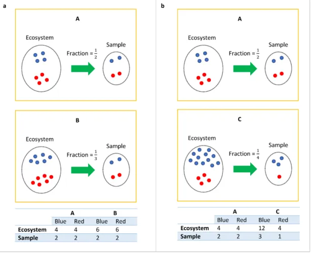
1 The bias introduced by cross-sample variations in sampling fractions. . . 4
2 Different alpha diversity measures using the diet swap data at the genus level. 9 3 Box plot of Rao’s quadratic entropy. . . 12
4 EM and WLS estimators of the bias term are highly correlated. . . 34
5 Box plot of residuals between true sampling fraction and its estimate. . . 44
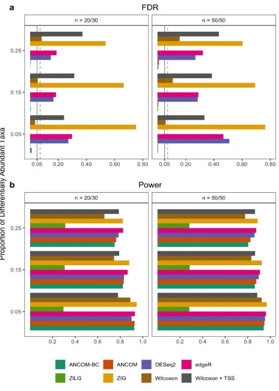
6 FDR and power comparisons using synthetic data. . . 45
7 FDR and power comparisons using global pattern data. . . 47
8 Non-metric multidimensional scaling (NMDS) visualizations of normalized data. 48 9 Analysis of the global gut microbiota data in phylum level. . . 49
10 FDR and power comparisons with small sample size. . . 54
11 FDR and power comparisons with large Prop. DA. . . 56
12 Graphs for ordered restrictions. . . 58
13 FDR and power comparisons for global test. . . 66
14 FDR and power comparisons for directional test. . . 66
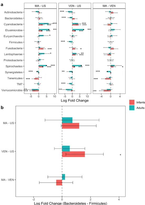
15 FDR and power comparisons for testing patterns (pattern matching ignored). 68 16 FDR and power comparisons for testing pattern (pattern matching considered). 69 17 Age effect on microbial absolute abundance of the global gut microbiota data. 71 18 Pairwise differential abundance analyses on locations using ANCOM-BC. . . 71
19 Relative abundance by location in phylum level. . . 72
20 Testing for patterns with respect to location effect. . . 73
21 Pearson correlation vs. Spearman correlation vs. Distance correlation. . . 76
22 Various kinds of associations between taxon 1 (T1) and Taxa 2 to 5 (T2 to T5). 77 23 Network visualizations for different correlation measures. . . 78
24 The relative abundances is the same between the ecosystem and sample. . . . 79
25 Distance correlations calculated by the original data vs. by ranks. . . 80
27 Network visualization of DICOM using synthetic data. . . 86 28 Implementation of DICOM using global gut microbiota data. . . 86
Preface
I would like to thank my advisors Dr. Peddada for his tremendous help and guidance in my dissertation. I really appreciate the opportunity of working with him and really enjoy the time we work together. I also want to express my gratitude to my committee members: Dr. Buchanich, Dr. Ding, Dr. Rogers, and Dr. Wang for their suggestions and comments for my dissertation work. Finally, I would like to thank all my family and friends for their constant support and encourage.
1.0 Introduction
Humans are estimated to have 45.6 million genes in oral and gut microbiome alone, which is about 2000-fold more genes than human genes (Tierney et al., 2019), therefore the microbiome is sometimes referred to as the ”second genome”, or another ”organ” of human body (O’Hara and Shanahan, 2006; Relman and Falkow, 2001; Hurst, 2017). It is hence not surprising that numerous diseases such as obesity (Turnbaugh et al., 2009), inflammatory bowel diseases (Gevers et al., 2014) and HIV (Lozupone et al., 2013a) are associated or even caused by changes in the microbial ecosystem. For these reasons, understanding changes in the composition of microbiome under different conditions is important for studying human diseases. A taxon is said to be differentially abundant between two ecosystems if its mean
absolute abundances in the two are significantly different. Estimation of absolute abundance of a taxon in a unit volume of an ecosystem based on a random sample of specimen from the ecosystem is a function of several factors such as the library size (the total number of sequencing reads for all taxa in a sample), microbial load (total number of absolute abundances for all taxa in a unit volume of an ecosystem), and the faction of the sample obtained from the ecosystem.
To reduce the ambiguity, throughout this dissertation, we use absolute abundance to denote count of a taxon regardless it is in a unit volume of an ecosystem (e.g. a patient’s intestine) or in a sample (e.g. a patient’s stool sample); whilerelative abundance is proportion of the absolute abundance of a taxon relative to the total absolute abundance of all taxa, thus it is between 0 and 1. For ease of exposition, various terms used in the literature are summarized in Table 1. The notations described in statistical methods are summarized in Table 2.
The next generation sequencing (NGS) technologies have made the analysis of high-dimensional microbiome data increasingly informative and feasible. There are two common approaches of sequencing performed to study the microbiome: (a) amplification and se-quencing of targeted genetic elements such as 16S rRNA gene in bacteria, or (b) shotgun metagenomics. While 16S rRNA sequencing is cost-effective and is very widely used (Amato,
Table 1: Definitions of key terminologies.
Term Definition
Microbiota Community of microscopic organisms. Microbiome Genes associated with the microbiota.
Amplicon Product of PCR amplification.
High-throughput Sequencing DNA sequencing approach that produces large amounts of sequence data rapidly at low cost.
OTU Operational taxonomic unit: Group of DNA
se-quences with 97% similarity.
SV Sequence variant: Individual DNA sequences
re-covered from a high-throughput marker gene analy-sis following the removal of spurious sequences gen-erated during PCR amplification and sequencing. Feature Table A matrix summarizing observed microbial absolute
abundances in the sample. Columns represent sam-ples and rows stand for OTUs or SVs.
Library Size The total number of (observed) absolute abun-dances for all taxa in a sample.
Microbial Load The total number of (unobserved) absolute abun-dances for all taxa in a unit volume of an ecosys-tem.
2017), its main drawback is that it can only identify bacteria. On the other hand, shotgun metagenomics surveys cover all given genomic DNAs, including DNAs from bacteria, viruses, and fungi. Additionally, shotgun metagenomic sequencing has greater taxonomy resolution (species - strains level of shotgun metagenomics vs. genus - species level of 16S sequencing), functional profiling, and it is less susceptible to biases that are inherent in targeted gene am-plification. However, as of today, metagenomic sequencing is substantially more expensive
Table 2: Summary of notations.
Notation Description
i Taxon index,i= 1,2, . . . , m. j Sample index,j = 1,2, . . . , n.
k Index of fixed effects, k = 1,2, . . . , p. l Index of Random effects,l = 1,2, . . . , q.
xjk The kth fixed effect of interest for the jth sample.
zjl The lth random effect of interest for the jth sample.
Aij‡ Unobserved absolute abundance ofith taxon in a unit volume of
ecosystem ofjth sample.
A·j‡ Microbial load in a unit volume of ecosystem ofjthsample. A·j =
Pm
i=1Aij.
γij‡ Unobserved relative abundance of ith taxon in a unit volume of
ecosystem ofjth sample.
Oij‡ Observed absolute abundance ofith taxon in a random specimen
taken from a unit volume of ecosystem of jth sample.
O·j‡ Library size of a random specimen taken from a unit volume of
ecosystem ofjth sample. O·j =
Pm
i=1Oij.
rij‡ Observed relative abundance of ith taxon in a unit volume of
ecosystem ofjth sample.
cj† For the jth sample, cj represents the proportion of its
ecosys-tem (unobserved absolute abundance) in a random specimen (ob-served absolute abundance), thus cj =
E(Oij|Aij)
Aij . We shall refer
to this constant as ”sampling fraction”.
yij‡ log(Oij).
dj† log(cj).
† Parameter; ‡ Random variable.
than 16S sequencing, and it may not be deep enough to detect the 16S rRNA genes of rare species in a community (Shah et al., 2011).
Figure 1: The bias introduced by cross-sample variations in sampling fractions.
The microbiome data are intrinsically compositional because the observed 16S rRNA gene data provides information in the form of relative abundances regardless of the microbial load of ecosystems(Fernandes et al., 2014; Mandal et al., 2015; Gloor and Reid, 2016; Gloor et al., 2016, 2017; Morton et al., 2017, 2019). Thus, they are constrained by a simplex (Aitchison, 1982). It is important to distinguish between absolute and relative abundances of taxa in a unit volume of an ecosystem. The choice of parameter for statistical analysis is important and needs to be clearly stated. Often researchers are interested in identifying taxa that are different in mean absolute abundance per unit volume between two or more ecosystems (Morton et al., 2019). Second, not all samples have the same sampling fraction.
For each taxon iwithin samplej, the sampling fraction is the ratio of the expected absolute abundance of taxoniwithin thejthsample (e.g. a stool sample) to its absolute abundance in
a unit volume of the ecosystem (e.g. gut) where the sample was derived from. The sampling fraction is constant for all taxa i within the jth sample. Thus the sampling fraction for the
jth sample is given by the following. Definition 1.0.1 (Sampling fraction).
cj =
E(Oij|Aij)
Aij
, (1.1)
where
(1) Oij is the observed absolute abundance of ith taxon in jth sample,
(2) Aij is the unobserved absolute abundance of ith taxon in the ecosystem ofjth sample,
(3) cj is the sample-specific sampling fraction.
The problem underlying the the differential abundance (DA) analysis of microbiome data is that while Oij is known, Aij is unknown and can vary drastically from sample to sample.
Consequently, the observed absolute abundances are not comparable between samples. The goal of DA analysis is to identify taxa whose absolute abundances, per unit volume, of the ecosystem (Aij) are significantly different with changes in the covariate of interest (e.g. the
group effect).
Consider the toy example in Figure 1, suppose the ecosystems (e.g. gut) of subject A, B and C consist of only two taxa, the blue and red taxa. A false negative may occur when comparing the ecosystems of A and B. Clearly, the true absolute abundance of each taxon is 50% more in subject B’s ecosystem as compared to subject A’s. However, they each have the same library size (4 each) in their respective samples (e.g. stool samples). Without considering the differential sampling fractions, one would falsely conclude that none of the taxa are differentially abundant in the two ecosystems. This erroneous conclusion would be avoided if one recognizes that we have a larger sampling fraction in the sample obtained from A’s ecosystem than from B’s (12 vs. 13). Similarly, we get a false positive result when comparing ecosystems of A and C. In their ecosystems, blue is more abundant in C than in A (12 vs. 4), and both have same amounts of red taxa (4 vs. 4). However, given that samples
from A and C have same library sizes, one may mistakenly conclude that both blue (2 vs. 3) and red taxa (2 vs. 1) are differently abundant between A and C. A third characteristic of feature table is that it is typically sparse, with as many as∼90% zero entries (Paulson et al., 2013), which creates a challenge for analyzing rare taxa. A quick and simple strategy to deal with excess zeros is to add a small positive constant (e.g. 1) called pseudo-count (Mandal et al., 2015; Xia et al., 2013) to each cell of the feature table. Even though adding a pseudo-count is simple and also widely used, the choice of the pseudo-pseudo-count is often ad-hoc. Other strategies involve modeling zero counts by some probability models (Paulson et al., 2013; Chen and Li, 2016). However, these methods may not be valid if the underlying parametric assumption does not hold. Instead of modeling zeros by parametric distributions, ANCOM-II512017Kaul et al. attempts to provide a general framework to classify and identify zeros into three different types, which includes outlier zeros caused by some extraneous reasons such as the wrong data entry, structural zeros because of the nature of the experimental groups, i.e. some bacteria are not expected to belong to certain environments (e.g. a desert) but in others (e.g. a rainforest), and sampling zeros owing to insufficient library size. In our opinion the zero counts problem is still an open problem and requires further investigation.
1.1 Measures of diversity
1.1.1 Alpha diversity
The alpha diversity (α-diversity) is a measure of diversity within a sample (Whittaker, 1960, 1972). One of the simplest and widely used measures to represent diversity isrichness
which is the number of taxa present in a sample (Magurran, 2013). Whereas, evenness is a measure of relative abundance of different taxa that make up the richness in that sample. Low values of evenness indicates that a small number of taxa dominate the composition, and high values indicates that relative abundances of different taxa are somewhat evenly distributed. For example, consider the guts of two 10-day old babies A and B. Suppose the stool sample from A has 10% Actinobacteria, 15% Bacteroidetes, 5% Proteobacteria and 70%
Firmicutes, and suppose the stool sample from B has 1% Actinobacteria, 0% Bacteroidetes, 5% Proteobacteria and 94% Firmicutes. In this example, eye-balling the relative abundances, we may conclude that baby A has higher evenness than baby B. Such eye-ball comparisons are not feasible when there are a large number of taxa. A variety of alpha diversity measures are available to quantify abundance and evenness. They can be broadly classified into two types, those that take into account the phylogenic relationships and those that do not. Some widely used non-phylogeny based metrics are Chao1 (Chao, 1984), Shannon’s diversity (Shannon, 1948) and Gini-Simpson’s index (Simpson, 1949). Among these, the latter two are commonly used in practice. These indices, take into account taxa’s richness, relative abundance and evenness(Morris et al., 2014).
A popular phylogeny based metric is Faith’s Phylogenetic Diversity (PD)(Faith, 1992) which is defined as follows.
Definition 1.1.1 (Phylogenetic diversity (PD)). As a quantitative measure of phylogenetic diversity, “PD” has been defined as the minimum total length of all the phylogenetic branches required to span a given set of taxa on the phylogenetic tree.
Unlike non-phylogeny based metrics, PD is a measure of biodiversity which incorporates phylogenetic difference among taxa. Phylogenetic patterns among taxa reflect general pat-terns of taxa variation at the level of genes or other features (Faith and Baker, 2006). Larger PD values are expected to correspond to greater feature diversity.
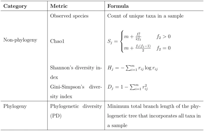
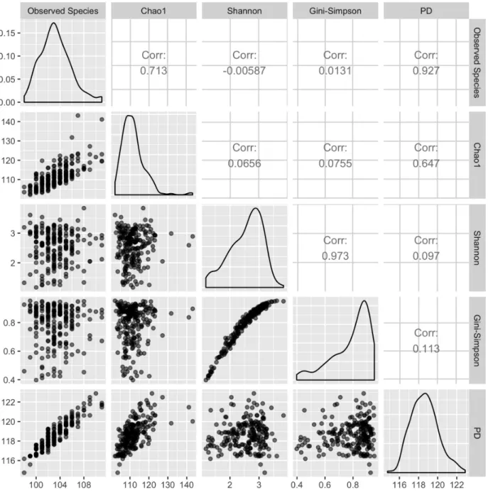
For convenience, the mentioned alpha diversity measures are summarized in Table 3. In Figure 2, we show different alpha diversity measures using the same data set, which is based on the two-week diet swap study between western (USA) and traditional (rural Africa) diets (O’Keefe et al., 2015). Note that since Shannon’s and Gini-Simpson’s diversity indices are based on similar principles, they are expected to be highly correlated in any given data set.
1.1.2 Beta diversity
Beta diversity (β-diversity) provides a measure of between-sample diversity, or distance or dissimilarity (Whittaker, 1960). When more than two samples are used, the beta diversity is calculated for every pair of samples to generate a distance/dissimilarity matrix. Similar
Table 3: Formulas for calculating alpha diversities.
Category Metric Formula
Non-phylogeny
Observed species Count of unique taxa in a sample
Chao1 Sj = m+ f12 2f2 f2 >0 m+ f1(f1−1) 2 f2 = 0
Shannon’s diversity in-dex Hj =− Pm i=1rijlogrij Gini-Simpson’s diver-sity index Dj = 1− Pm i=1r2ij
Phylogeny Phylogenetic diversity (PD)
Minimum total branch length of the phy-logenetic tree that incorporates all taxa in a sample
Note that:
(1) f1 = number of singletons (taxon appear once) in the sample,
(2) f2 = number of doubletons (taxon appear twice) in the sample.
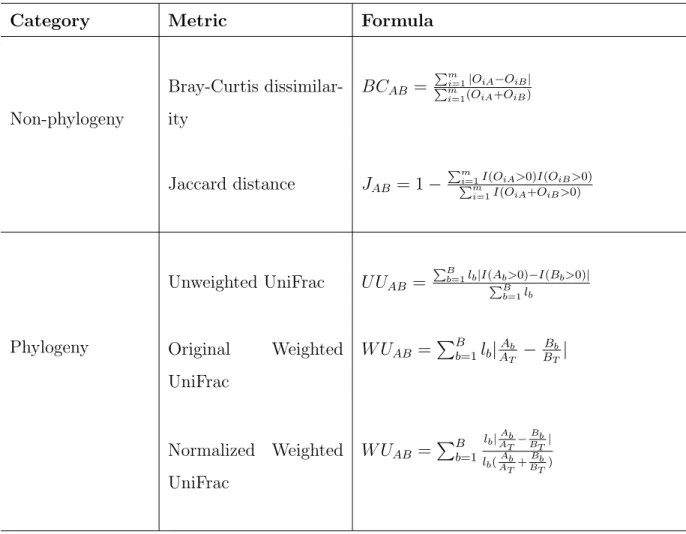
to alpha diversity, the beta diversity can be categorized into non-phylogeny based metrics, such as Bray-Curtis dissimilarity (Bray and Curtis, 1957), Jaccard distance (Jaccard, 1901), and phylogeny based metrics such as Unweighted UniFrac (Lozupone and Knight, 2005) and Weighted UniFrac (Lozupone et al., 2007). For simplicity of exposition, suppose we have two samples, i.e. sample A and B, the mentioned beta diversity measures are summarized in Table 4.
Among non-phylogeny based beta diversities, Bray-Curtis dissimilarity is constructed using the observed absolute abundance (count data) and it ranges from 0 to 1, with 0 corresponding to the case when A and B have identical observed absolute abundance of all
Figure 2: Different alpha diversity measures using the diet swap data at the genus level.
taxa, and 1 corresponds to the case when the two samples have complete different observed absolute abundances. Thus larger value correspond to more diversity between samples. On the other hand, Jaccard distance is a dissimilarity measure for presence or absence of taxa
Table 4: Formulas for calculating beta diversities.
Category Metric Formula
Non-phylogeny Bray-Curtis dissimilar-ity BCAB = Pm i=1|OiA−OiB| Pm i=1(OiA+OiB) Jaccard distance JAB = 1− Pm i=1I(OiA>0)I(OiB>0) Pm i=1I(OiA+OiB>0) Phylogeny Unweighted UniFrac U UAB = PB b=1lb|I(Ab>0)−I(Bb>0)| PB b=1lb Original Weighted UniFrac W UAB = PB b=1lb|AATb −BBTb| Normalized Weighted UniFrac W UAB = PB b=1 lb|ATAb−BTBb| lb(ATAb+BTBb) Note that:
(1) I(Oij >0) is the indicator function which equals to 0 or 1 as taxon i is absent
or present in sample j,
(2) B = the total number of branches in the phylogenetic tree, (3) lb = the length of branchb,
(4) jb = total number of descendants of branch b from sample j,
(5) I(jb >0) = indicator equal to 0 or 1 as descendants of node babsent or present
in samples j.
without taking into account the abundance information. It ranges from 0 to 1, with 0 implies that the two samples share exact the same taxa, and 1 implies there is no common taxa.
The larger value the more diverse the data.
Unweighted UniFrac and Weighted UniFrac are two popular phylogeny based diversity measures which are calculated using sequence distances in the phylogenetic tree. They are based on the fraction of branch length that is shared between two samples or unique to one or the other sample. Unweighted UniFrac is purely based on sequence distances so it does not include abundance information, while Weighted UniFrac includes both sequence and abundance information by weighting branch lengths using relative abundances. Unweighted UniFrac and (Normalized) Weighted UniFrac range from 0 to 1, the larger value corresponds to larger diversity.
1.1.3 Analysis of Diversity (ANODIV)
While the alpha and beta diversities are well studied in the microbiome literature, Rao’s Quadratic Entropy (Rao, 1984; Nayak, 1986; Ricotta and Marignani, 2007; Rao, 2010; Chen et al., 2018) and the resulting Analysis of Diversity (ANODIV) has not been well discussed in the microbiome literature. The ANODIV resembles the classical ANOVA but is based on diversity measures. Although a variety of diversity measures may be used in defining quadratic entropy, for simplicity of exposition, in this paper we shall use Gini-Simpson index when defining Rao’s quadratic entropy. In practice one may consider more informative mea-sures depending on the available information and scientific question. Analogous to ANOVA, the ANODIV provides a general framework for analyzing complex designs including multi-factorial studies with covariate adjustments (Nayak, 1986), (Rao, 2010). As demonstrated in (Rao, 2010) the total diversity (SST) can be partitioned into various components such as within group (SSW) and between group (SSB), which can be further decomposed into other components depending upon the study design. Based on the asymptotic theory developed in (Nayak, 1986), one can formally test the null hypothesis that the compositions of two or more ecosystems are same. Thus, the classical machinery of ANOVA or ANCOVA can be easily imported into ANODIV. Although, mathematically, the asymptotic theory developed by Nayak (Nayak, 1986) is designed for the case when the sample sizes are larger than the number of taxa, there is an opportunity to extend those results for high-dimensional
mi-crobiome data. If the analysis are carried out at higher order of the phylogeny, say at the phylum or class or perhaps even order level, where the sample sizes might be larger than the number of taxa (i.e. phylum, class or order) then ANODIV can be applied directly.
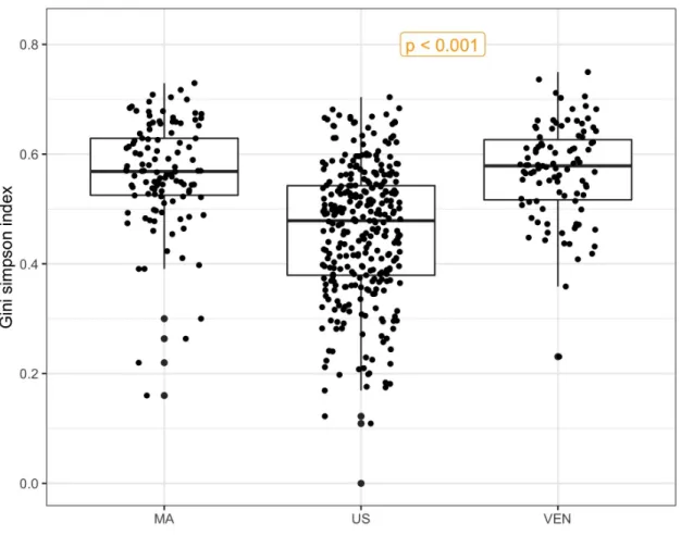
Figure 3: Box plot of Rao’s quadratic entropy.
Let ˆPg = ( ˆPg1,Pˆg2, . . . ,Pˆgm)T denote the sample proportions ofm taxa in thegth group,
which are estimated using ng observations in the gth group, g = 1,2, . . . , G. Let ˆP. denote
the weighted average of ˆP1,Pˆ2, . . . ,PˆG, weights being the sample sizes n1, n2, . . . , nG. For a
vector of proportionsP, defineH(P) = PT∆P, where ∆ is a suitably chosenm×m matrix.
For example, in the case of Gini-Simpson index, which is used in this paper, ∆ =J −I, J is a matrix where all elements are 1 and I is the identity matrix. Then the total diversity is defined as SST = H( ˆP.) and within-sample diversity is SSW = PGg=1 nngH( ˆPg) and the
between sample diversity is SSB =SST −SSW =−PG
g=1
ng
n( ˆPg−Pˆ.) T∆( ˆP
g −Pˆ.). Note
non-negative. Under the null hypothesis that all populations have same relative abundance of all taxa, the asymptotic distribution of (g−1)(n−1)SSB/SST is central χ2
(g−1)(m−1).
To illustrate ANODIV, we use the global gut microbiota data (Yatsunenko et al., 2012) and analyze it at the phylum level. Using data on 39 phyla with subjects from Malawi (MA, n1 = 114), USA (US, n2 = 317), and Venezuela (VEN,n3 = 99), we found the total diversity
(SST) in the three samples to be 0.574, the within sample diversity SSW = 0.567, and the between sample diversity SSB = 0.007, with a p-value of 4.30×10⁻¹⁸, we reject the null hypothesis that the phyla compositions are same among the three countries. The box plot in Figure 3 seems to confirm this finding. Although the variation within each box is very large, which seems to be consistent with very large SSW, and numerically SSB is small, three box plots appear to be significantly different, and the statistical test is sensitive to find a statistically significant p-value. Thus the ANODIV is a useful method to test hypotheses regarding the equality of microbial compositions in two or more groups.
1.2 Differential abundance analysis
1.2.1 Normalization methods
As we described intuitively in the introduction, a main obstacle for performing DA analysis is the unknown sampling fractions. Therefore, normalization is critical to enable meaningful comparison of absolute abundances from different experimental conditions by eliminating artificial biases caused by the variability of sampling fractions. The primary objective of normalization is to transform the observed absolute abundances in samples so that expected differences in the mean absolute abundances between two ecosystems is not confounded by the differences in the sampling fractions. Thus correcting for the bias induced by differential sampling fractions should be an important objective of a normalization procedure. Failure to do so will result in a systematic bias that increases the false discovery rate (FDR) and loss of power.
studies. It was first recommended for microbiome data in order to moderate differences in the presence of rare taxa (Lozupone et al., 2011). Rarefaction curves represent the diversity as a function of library sizes. If the lines in the plot appear to “level out” (i.e., approach a slope of zero) at some library size along the x-axis, that suggests that the diversity of the samples has been fully observed or sequenced. Otherwise, increasing the minimum library size would be likely to result in the observation of additional features. Originally, the diversity metrics used in rarefaction curves was alpha diversity (Gotelli and Colwell, 2001; Brewer and Williamson, 1994). However, recent years have seen studies using beta diversities (Horner-Devine et al., 2004; Jernvall and Wright, 1998) as well. Although rarefaction has been criticized for potential loss of statistical power when a relatively large proportion of data is removed, some studies (Weiss et al., 2017) have demonstrated that it remains to be a promising technique for ordination/clustering and that control of false positive rate due to rarefaction outweighs any loss in power.
Scaling the data is another popular method of normalization of microbiome data. The basic idea is to multiply each element in the feature table by a ”normalization factor” to eliminate biases resulting from unequal sampling fractions. Some commonly used normal-ization methods include Cumulative-Sum Scaling (CSS) implemented in metagenomeSeq (Paulson et al., 2013), Median (MED) in DESeq2 (Love et al., 2014), Upper Quartile (UQ) (Bullard et al., 2010) and Trimmed Mean of M-values (TMM) (Robinson and Oshlack, 2010) in edgeR (Robinson et al., 2010), Wrench (Kumar et al., 2018), and Total-Sum Scaling (TSS) that simply transforms the abundance table (feature table) into relative abundance table, i.e. scale by each sample’s library size. Note that as stated in the user manual of edgeR (Chen et al., 2014), the author suggests that to address the ”RNA composition” effect, one should multiply the normalization factors with the corresponding library size to account for “effective library size”. Hence, we also considered modified versions of UQ and TMM, de-noted as ”ELib-UQ” (Effective library size using UQ) and ”ELib-TMM” (Effective library size using TMM) in this paper. Since the literature is not often very explicit regarding the mathematical formulas used by various methods, we provide some useful formulas in Table 5.
Table 5: Summary of different normalization methods.
Method Sampling Fraction Estimate
ANCOM-BC log(ˆcANCOM-BCj ) = m1 Pm
i=1(yij−xTjβˆi) CSS ˆcCSSj = s ˆ l j+1 N MED ˆcMED j = median i:OR i 6=0 Oij OR i UQ ˆcUQj = UQ i:Oij>0 (Oij O·j) TMM log2(ˆcTMMj ) = P i∈G∗wijMij P i∈G∗wij Elib-UQ ˆcElib-UQj =O·jˆcUQj Elib-TMM ˆcElib-TMMj =O·jˆcTMMj Wrench ˆcWrench j = 1 m Pm i=1bij rij ¯ ri· TSS ˆcTSSj =O·j Where
(1) ˆβi is obtained from ANCOM-BC algorithm,
(2) N = an approximately choose normalization constant, (3) sˆl j = P i:Oij≤q ˆ l j Oij, (4) qˆl j = ˆlth quantile of sample k, (5) ORi = (Qn j=1Oij) 1 n,
(6) UQ(X) denotes the upper quartile of X, (7) Mij = log2(
Oij
O·j)−log2(
Oij0
O·j0), where j
0 is the reference sample,
(8) wij =
O·j−Oij
O·jOij +
O·j0−Oij0
O·j0Oij0 , wherej
0 is the reference sample,
(9) G∗ represents a set of taxa that were not considered as extreme data for fold-change (M values) and average intensity (A values).
et al., 2013) since a few preferentially sampled measurements (e.g. taxa, genes) will have an undue influence on the relative abundance data. Change in the abundance of a single taxon can alter the relative abundances of all taxa. The Cumulative-Sum Scaling (CSS) (Paulson et al., 2013) in metagenomeSeq modifies Total-Sum Scaling (TSS) in a sample-specific manner to reduce biases resulting from preferentially sampled taxa. CSS assumes that read counts of all samples should be roughly independent and identically distributed up to a specific quantile. The Median normalization (MED) method used in DESeq2 (Love et al., 2014) assumes that a large proportion of taxa are not differentially abundant. While this may be a reasonable assumption in gene expression studies where most genes are not differentially expressed, but in the case of microbiome data it is not a reasonable assumption. Depending upon the application, a very large proportion of taxa may be differentially abundant between two conditions. The Upper Quartile normalization (UQ) and the Trimmed Mean of M-values (TMM) used in edgeR have similar issues as MED in DESeq2. UQ assumes that the upper quartile can capture the invariant segment of the count distribution, however, choosing the most effective quantile is nontrivial (Paulson et al., 2013; Robinson et al., 2010; Bullard et al., 2010; Dillies et al., 2013; Anders and Huber, 2010; Agresti and Hitchcock, 2005). Similarly, TMM is based on the hypothesis that most taxa are not differentially abundant. The scaling factor is calculated using a weighted trimmed mean of log absolute abundance ratios by first trimming (by default) the taxa belong to upper and lower 30% M values (taxon-wise log-fold-change) or 5% A values (absolute abundance level). Wrench (Kumar et al., 2018) assumes the observed absolute abundances are from a hurdle Log-Gaussian distribution. A robust location estimate of the Gaussian distribution leads to the desired scaling factor for each sample. However, Wrench currently implements strategies for categorical variable only, and the estimated scaling factor is essentially the average of ratios of relative abundances across taxa, which implicitly requires that most taxa do not change across conditions, or the effect sizes of differentially abundant taxa are not too large. One must exercise caution when using scaling methods as well. Most importantly, a scaling method is likely to overestimate or underestimate the fractions of zero counts depending on the corresponding library size of each sample (Friedman and Alm, 2012; Agresti and Hitchcock, 2005). This problem becomes more obvious for microbiome data since its feature table is typically sparse.
In this dissertation, we proposed a novel method called Analysis of Compositions of Microbiome with Bias Correction (ANCOM-BC), which will be discussed in detail in the next two chapters, it assumes that the observed sample is an unknown fraction of a unit volume of the ecosystem, and the sampling fraction varies from sample to sample. ANCOM-BC accounts for sampling fraction by introducing a sample-specific offset term in a linear regression model that is estimated from the observed data. The offset term serves as the bias correction.
Finally, Aitchison’s log-ratio transformation (Aitchison, 1982) implemented in in methods such as ALDEx2 (Fernandes et al., 2014), ANCOM (Mandal et al., 2015), and DR (Morton et al., 2019), is another alternative normalization method for compositional data. By taking log-ratios on observed absolute abundances or relative abundances within each sample, one is eliminating the effect of sampling fraction inherent to a given sample. There are three obvious choices for the log-ratio transformation, described below:
Definition 1.2.1 (additive log-ratio transformation (alr) (Aitchison, 1982), Sm →Rm−1).
alr(Oj) = [log( O1j Oi0j ), . . . ,log(Omj Oi0j )], (1.2) where
(1) Oj is the observed absolute abundances for sample j,
(2) i0 is taken to be the reference taxon.
Since alr projects the observed absolute abundances, which originally reside in a m di-mensional simplex, intom−1 dimensional Euclidean space, standard calculus of Euclidean geometry becomes valid. Note that alr transformation is an isomorphism, but not isometry, meaning that distances on transformed values will not be equivalent to distances on the orig-inal compositions in the simplex. One apparent drawback with alr is the choice of reference taxon (Morton et al., 2019). For different reference taxa, one gets different interpretations of the data.
The ambiguity of the chosen of reference taxon can be reduced by selecting the center-of-mass as the reference, allowing a one-to-one transformation of all taxa. This can be achieved by the so-called centered log-ratio transformation (clr):
Definition 1.2.2 (centered log-ratio transformation (clr) (Aitchison, 1982), Sm → Um). clr(Oj) = [log( O1j g(Oij) ), . . . ,log( Omj g(Oij) ], (1.3) where
(1) Oj is the observed absolute abundances for sample j,
(2) g(x) is the geometric mean of x, (3) Um ={[u
1, . . . , um] :u1+. . .+um = 0} is a hyperplane ofRm.
This transformation to a real space again makes the implementation of unconstrained statistical methods possible. clr transformation is an isometry, but sum of the transformed values equals to 0, leading to a degenerate distribution.
Neither alr nor clr transformation can be directly linked to an orthogonal coordinate system in the simplex. The isometric log-ratio transformation (ilr) (Egozcue et al., 2003) transformation (also known as balance), which is an isometry betweenSmand
Rm−1, provides
a solution to this problem.
Definition 1.2.3 (isometric log-ratio transformation (ilr), Sm →Rm−1).
ilr(Oj) = clr(Oj)ΨT, (1.4)
where
(1) Oj is the observed absolute abundances for sample j,
(2) Ψ is a (m−1, m)-matrix of basis.
There are multiple ways to construct orthonormal bases. Typically, if a bifurcating tree is given then we can construct a basis from the internal nodes in the tree, where each element in the ilr transformed data is of the following form:
bj = s |jL||jR| |jL|+|jR| log[g(jL) g(jR) ], (1.5) where
(1) bj is the balance at internal node j,
(3) jR is the set of relative abundances contained in the right subtree at internal nodej ,
(4) |jL| is the number of taxa contained in jL,
(5) |jR| is the the number of taxa contained injR,
(6) g(x) is the geometric mean of x.
One caveat of applying log-ratio transformation is the choice of pseudo count. Because of the nature of log transformation, the addition of a pseudo count is necessary to handle sampling zeros. Studies have shown that differential abundance or clustering results could be sensitive to the choice of pseudo count (Costea et al., 2014; Paulson et al., 2014). Although different values of pseudo count have also been exhaustively discussed (Egozcue et al., 2003; Costea et al., 2014; Paulson et al., 2014; Greenacre, 2011), to our best knowledge, there is no consensus on how to choose the optimal value.
1.2.2 Methods of differential abundance analysis
One of the objectives in this dissertation is to identify taxa that are differentially abun-dant between two or more groups, and determine the biological functions and processes associated with such taxa. A number of procedures have been introduced and used in the literature for identifying differentially abundant taxa.
One common approach is to apply a nonparametric test (e.g. the Mann-Whitney test for two groups; the Kruskal-Wallis test for multiple groups) after rarefying the feature table. Un-fortunately, these standard nonparametric tests do not take into account the compositional structure of microbiome data.
As alternatives to standard nonparametric tests, many parametric models have been proposed in the literature based on transcriptomics data such as RNA-Seq data for testing differences across experimental groups. Among them, DESeq2 (Love et al., 2014) and edgeR (Robinson et al., 2010) are two most popular methods. They both model the count data using negative binomial distributions to allow for extra variation, and use shrinkage estimation for dispersions to improve stability and reliability of estimates.
1.2.2.1 RNA-seq based methods: DESeq2 and edgeR Both DESeq2 and edgeR model the observed absolute abundances using the negative binomial distribution. While both methods are in general very reasonable and appropriate for gene expression data, they seem to perform poorly for microbiome data. This is largely because, as stated earlier, the normalization methods used by these two methods intrinsically assume that a very small fraction of taxa are deferentially abundant. This assumption is not valid for microbiome data. As a consequence, the test statistics used by these methods are biased under the null hypothesis. As demonstrated in several previous studies (Mandal et al., 2015; Weiss et al., 2017), the bias in the test statistic results in inflated FDRs for these methods. What is worse, as the sample size increases, the FDR increases for these methods.
1.2.2.2 MetanegomeSeq Instead of using a negative binomial model, metagenomeSeq
(Paulson et al., 2013) used a zero-inflated Gaussian mixture (ZIG) model, with the zero mass tackling excess zeros due to insufficient sequencing depth or biological nature, and the Gaussian distribution modeling the non-zero counts. However, as shown in simulation studies (Weiss et al., 2017), metagenomeSeq was the only method, among all parametric models, that increased FDR when using rarefied data. This might due to its zero-inflated model which requires the raw library size to capture the zero proportion. Even with its own normalization method (CSS), metagonomeSeq still has a highly inflated FDR, and it gets worse when sample size or the fold change increases (Mandal et al., 2015; Weiss et al., 2017). The authors of metagenomeSeq, modified their procedure and recommend using zero-inflated Log-Gaussian (ZILG) mixture model instead of zero-zero-inflated Gaussian (ZIG) mixture model for each feature. Although this improves the FDR control, the procedure becomes extremely conservative, with FDR close to zero and substantial loss in power.
1.2.2.3 ALDEx2 Inherited from the original version of ANOVA-Like Differential Ex-pression (ALDEx) analysis (Fernandes et al., 2013), ALDEx2 was proposed as a compo-sitional data analysis tool that is applicable to three different types of data: RNA-Seq, ChIP-Seq and 16S rRNA sequencing (Fernandes et al., 2014). By acknowledging these high-throughput sequencing datasets are fundamentally compositional, the methodology of
ALDEx2 can be summarized as follows:
(1) The observed absolute abundances are converted to relative abundances by Monte Carlo (MC) sampling from the Dirichlet distribution with the addition of a uniform prior. The MC sampling is repeated for K times (K = 128 times by default), thus essentially, for each taxon iin samplej, the observed absolute abundanceOij is represented by a vector
of MC samples of relative abundances (rij(1), . . . , rij(K))T,
(2) Within each sample j and each MC Dirichlet realization k, k = 1, . . . , K, the relative abundances (r(1kj), . . . , rmj(k))T is clr transformed giving a vector of transformed values, (3) Significance test (Welch’s t-test or Wilcoxon test) is performed on each taxon in the
vector of clr transformed values. Since there are a total of K MC Dirichlet samples, each taxon will result in K p-values.
(4) Each resulting p-value is corrected using the B-H71995Benjamini and Hochberg procedure, and
the expected adjusted p-value for each taxon is reported by taking the empirical mean of K adjusted p-values.
The ALDEx2 was designed to identify differential abundances of features (genes, taxa, or genomic segments) between two or more sample groups, relative to the geometric mean absolute abundance. Thus, the parameter of interest in ALDEx2 is different from the pa-rameter of interest in DA analysis. Throughout this dissertation, a differentially abundant taxon is the one whose mean absolute abundance in the ecosystem is significantly different with regard to the covariate of interest. As a result, ALDEx2 not only generally exceeds the nominal level of FDR (5%), but also has substantially smaller power as compared to competing DA methods (Morton et al., 2019).
1.2.2.4 Analysis of composition of microbiomes (ANCOM) is an Aitchison’s
log-ratio based methodology (Aitchison, 1982), which accounts for the compositional structure of microbiome data. Suppose there are a total of m taxa, ANCOM relies on two mild assumptions as follows. Under these assumptions, the authors proved that one can test the null hypotheses regarding absolute abundance in a unit volume using relative abundances.
Assumption 1.2.1. The mean abundance (in log scale) of at most m−2taxa are different. Thus, some two taxa are assumed to be not differentially abundant.
Assumption 1.2.2. The mean abundance (in log scale) of all m taxa do not differ by the same amount between the two study groups.
For theith taxon andjthsample, the ANCOM uses standard ANOVA model formulation:
log r (g) ij r(i0gj) =αii0 +β(g) ii0 + X k xjkβii0k+(g) ii0j, (1.6)
where i0 is the reference taxon, i0 6=i= 1,2, . . . , m, g = 1,2, . . . , G is the number of groups, αii0 is the overall common mean, β(g)
ii0 is factor of interest at the gth level, xjk are adjusting
covariates indexed by k. (iig0)j ∼N(0, σii20).
By virtue of Assumption 1.2.1 and Assumption 1.2.2, to test whether a taxon iis differ-entially abundant according to a factor of interest with G levels, it is equivalent to test:
H0(ii0) :β(1) ii0 =. . .=β (G) ii0 = 0, H1(ii0) : Not all β(g) ii0 equals to 0, for every i6=i0.
Altogether m(m2−1) distinct null hypothesesH0(ii0),i6=i0are tested using a multiple testing
correction such as the Benjamini-Hochberg (BH) procedure (Benjamini and Hochberg, 1995). For each taxon, the number of rejections, denoted asWi, is counted, and ANCOM makes use
of the empirical distribution of{W1, W2, . . . , Wm}to determine the cut-off value of significant
taxon. The rule of thumb is when the value of Wi is larger, it is more likely that taxon i
tends to be differentially abundant. The author recommends using 70 percentile of the W distribution as the empirical cut-off value.
As shown by simulation studies (Mandal et al., 2015; Weiss et al., 2017), ANCOM suc-cessfully controls the FDR under the nominal level (5%) while maintaining adequate power. However, ANCOM can be computationally intensive especially if the number of taxa is large. In addition, the statistical decision made by ANCOM depends on the quantile of its test statistic rather than quantitative measures such p-values, which some biologists find it difficult to interpret.
1.2.2.5 Differential Ranking (DR) exploits the fact that the ranks of relative differ-entials are identical to the ranks of absolute differdiffer-entials. They estimate relative differdiffer-entials using a multinomial regression where OTUs/SVs are the explanatory variables in the model. The regression coefficients corresponding to different taxa are ranked in order to determine the most important to least important taxa.
The multinomial regression model is formulated using additive log-ratio (ALR) transfor-mation: βik ∼N(0, µβ) ηj = alr −1 (βiTxj) O·j ∼Multinomial(ηj), (1.7)
The model parameters are estimated using a maximum a posteriori priori (MAP) estimation by stochastic gradient descent. Since the regression parameters are estimated under the constraint that they sum to 0, this method does not require to pre-specify the reference taxon and hence is robust to the choice of reference taxon. Secondly, it does take into account the compositional structure of microbiome data.
Note that, unlike other methods which use ap-value, this method makes decisions solely on the magnitude ofβik and the ranks of taxa derived from there.
1.2.2.6 Gneiss (Morton et al., 2017) is different from all above DA methods in the sense that it aims to move away from identifying differential abundance properties of individual taxon; Instead, in its implementations, it explore the concept of balances (Egozcue and Pawlowsky-Glahn, 2005; Pawlowsky-Glahn and Egozcue, 2011) to infer meaningful proper-ties of sub-communiproper-ties. It is important to note that gneiss is not designed to infer changes of absolute abundance for each individual taxon, but it can limit the number of possible scenarios with regards to the absolute changes of a group of taxa.
2.0 Analysis of Compositions of Microbiomes with Bias Correction (ANCOM-BC)
2.1 Introduction
As introduced in the last chapter, a number of procedures have been proposed and used in the literature for identifying deferentially abundant taxa between two or more ecosystems. A detailed survey of some of the existing methods and their performance has been discussed in (Weiss et al., 2017). As noted in a list of studies (Mandal et al., 2015; Gloor and Reid, 2016; Gloor et al., 2016, 2017; Morton et al., 2019), the observed microbiome data are relative abundances, hence they are compositional. Standard statistical methods are not appropriate for analyzing compositional data (Aitchison, 1982). Methods such as ANOVA, Kruskal-Wallis test do not appropriately take into consideration the compositional feature of microbiome data when performing differential abundance (DA) analysis. As demonstrated in literatures (Weiss et al., 2017; Mandal et al., 2015), these methods are subject to inflated false discovery rates (FDR). Although metagenomeSeq (Paulson et al., 2013) was specifically developed for microbiome data, it too is subject to inflated FDR under the Gaussian mixture model (Weiss et al., 2017; Mandal et al., 2015).
Aitchison’s methodology converts relative abundances, which are points in a simplex (i.e. compositional), into points in a lower dimensional Euclidean space by taking suitable log-ratios of each taxon with respect to a pre-specified reference taxon or the geometric means of all taxa. However, there are two caveats to keep in mind when using this class of methods (Morton et al., 2019). Firstly, the results and interpretation of data depend on the reference frame. Secondly, some of these methods are appropriate for relative abundance and not the absolute abundance(Morton et al., 2019). Although ANCOM (Mandal et al., 2015) uses Aitchison’s framework, it is important to remind that unlike other compositional methods, in its implementation, the ANCOM algorithm does not fix one single taxon (or the geometric mean) as a reference, but uses all taxa and pools results from all such analyses when declaring differential abundance of a particular taxon. Thus, the reference taxon issue
(Morton et al., 2019) does not apply to ANCOM. By assuming that the mean absolute abundance of two taxa are not different between two ecosystems, ANCOM (Mandal et al., 2015) developed a strategy that enables researchers to infer about mean absolute abundances by testing hypotheses regarding mean relative abundances. Thus, unless the absolute mean abundance of almost all taxa changed, ANCOM should perform well in terms of FDR and power. One of the deficiencies of ANCOM is that it does not provide p-value for individual taxon, nor can it provide standard errors or confidence intervals of differential abundance for each taxon, and it can be computationally intensive. According to an extensive simulation study (Weiss et al., 2017), among the available methods for DA analysis, only ANCOM performs well in controlling FDR at the desired level while maintaining high power, as long as the sample size is not too small (e.g. n = 5 per group).
The Differential Ranking (DR) methodology (Morton et al., 2019) reformulates the prob-lem as a multinomial regression probprob-lem. By imposing the constraint that sum of the regres-sion coefficients is zero, the DR methodology accounts for compositionality in the relative abundance of microbiome data. Thus, unlike ALDEX2 (Gloor, 2015), they do not require the pre-specification of a reference frame. This makes their method more flexible than ALDEX2. Also, as demonstrated in their paper (Morton et al., 2019), the ranks of relative differentials perfectly correlate with ranks of absolute differentials. This result is consistent with the analytical results obtained by ANCOM, provided 2 taxa are not differentially abundant (in mean absolute abundance). Similar to ANCOM, the DR procedure does not provide explicit p-values or confidence intervals to declare statistical significance.
Since not all samples have the same sampling fraction, all DA methodologies require the counts to be properly normalized to account for differences in sampling fractions across samples. Sampling fraction is determined by two components, namely, the microbial load in a unit volume of the ecosystem (e.g. gut) and the library size of the corresponding sample (e.g. total species abundance sequenced from a subject’s stool sample). Therefore it is not sufficient to normalize the library size across samples as one needs to take into consideration the differences in the microbial loads. As shown in Figure 1, if a normalization method is based only on the library size and ignores the sampling fraction, then the two samples (A and B) would be considered as normalized, which leads to a false negative conclusion. Thus,
normalizing data on the basis of sampling fractions gives a better description of the truth than normalization methods that rely purely on the library sizes.
Ideally, under the null hypothesis, the test statistic for DA analysis should be (at least approximately) centered at zero (i.e. unbiased). However, for many DA methods, this is not always true for at least one of the following reasons: (1) The test statistic may not be designed for testing hypothesis regarding the actual parameter of interest. For example, the statistic is designed to test hypotheses regarding relative abundance but the null hypothesis is regarding the absolute abundance; (2) Data are not properly normalized. For example, data are normalized to correct for differences in library sizes only but not account for differences in the sampling fractions; (3) Underlying structure, such as compositionality, is ignored; (4) The methodology imposes strong parametric assumption on the data, which could lead to a potential model misspecification problem. For instance, although DESeq2(Love et al., 2014) and edgeR(Robinson et al., 2010) have been widely used for DA analysis, studies on RNA-Seq data have shown that they could yield high FDR as the negative binomial model does not fit the data well when there are many zeros (Weiss et al., 2017). Applying non-parametric tests, such as Wilcoxon rank-sum test, to the OTU table directly, not only neglects the compositional structure of the absolute abundance data, but also implicitly assumes equivalent sampling fractions for all samples.
Motivated by the above reasons, in this chapter we propose a novel methodology called Analysis of Compositions of Microbiomes with Bias Correction (ANCOM-BC) that 1) ex-plicitly tests for differential absolute abundance, 2) normalizes the OTU table for differences in sampling fractions among samples, 3) account for the compositional structure of the OTU table properly, and 4) does not make strong parametric assumptions on the data. As in ANCOM and DR, ANCOM-BC assumes that the observed sample is an unknown fraction of a unit volume of the ecosystem, and the sampling fraction varies from sample to sample. ANCOM-BC accounts for sampling fraction by introducing a sample-specific offset term in a linear regression model, that is estimated from the observed data. The offset term serves as the bias correction, and the linear regression framework in log scale is analogous to log-ratio transformation to deal with the compositionality of microbiome data. The case of zero counts is also discussed in Methods section. This methodology has some conceptual
similar-ities with DR, but is fundamentally different. With ANCOM-BC, one can perform standard statistical tests and construct confidence intervals for differential abundance. Moreover, as demonstrated in benchmark simulation studies, ANCOM-BC (a) controls the FDR very well while maintaining adequate power compared to other popular methods, and (b) it is sub-stantially faster the ANCOM. The CPU time is 0.28 mins vs 63 mins when the number of taxa is 500. The CPU time for ANCOM increases dramatically as the number of taxa increases to 1,000. In this case, the CPU times for ANCOM-BC and ANCOM are 0.51 mins and 211 mins, respectively. In addition to results based on synthetic data, we also illustrate ANCOM-BC using the well-known global gut microbiota dataset (Yatsunenko et al., 2012).
2.2 Methods 2.2.1 Model assumptions Assumption 2.2.1. E(Oij|Aij) =cjAij, V ar(Oij|Aij) = σ2w,ij, (2.1) where σ2
w,ij = variability between specimens within the jth sample. Therefore, σw,ij2
char-acterizes the within-sample variability. Typically, researchers do not obtain more than one specimen at a given time in most microbiome studies. Consequently, variability between specimens within sample is usually not estimated. Throughout this paper, we use ”sample” and ”specimen” exchangeably.
According to Assumption 2.2.1, in expectation the absolute abundance of a taxon in a random sample is in constant proportion to the absolute abundance in the ecosystem of the sample. In other words, the expected relative abundance of each taxon in a random sample is equal to the relative abundance of the taxon in the ecosystem of the sample.
Assumption 2.2.2. For each taxon i, Aij, j = 1, . . . , n, are independently distributed with
E(Aij|bi, xj) =bTi xj,
V ar(Aij|bi, xj) =σb,ij2 ,
where
(1) xj = (xj1, xj2, . . . , xjp)T are the covariates of interest for the jth sample, (2) bi = (bi1, bi2, . . . , bip) are the corresponding coefficients for xj,
(3) σb,ij = between sample variation for the ith taxon.
The Assumption 2.2.2 states that for a given taxon, all samples are independent.
2.2.2 ANCOM-BC for fixed effects models
2.2.2.1 Regression framework From Assumptions 2.2.1 & 2.2.2, we have:
E(Oij|bi, xj) = cjbTi xj, V ar(Oij|bi, xj) = f(σw,ij2 , σ 2 b,ij) :=σ 2 t,ij. (2.3)
Motivated by the above set-up, we introduce the following linear model framework for log-transformed absolute abundances:
yij =dj +βiTxj +ij, (2.4)
with
E(ij) = 0,
E(yij) = dj+βiTxj,
V ar(yijk) =V ar(ijk) :=σij2.
(2.5)
Note that the above log-transformation of data is inspired by the Box-Cox family of trans-formations (Box and Cox, 1964) which are routinely used in data analysis.
Rewrite the model (2.4) in the vector form, we have
with E(i) = (0, . . . ,0)T, E(yi) =d+Xβi, Cov(yi) = Cov(i) = σ2 i1 0 . . . 0 0 σi22 . . . 0 .. . ... . .. ... 0 0 . . . σin2 . (2.7) where (1) yi = (yi1, yi2, . . . , yin)T, (2) d= (d1, d2, . . . , dn)T, (3) βi = (βi1, βi2, . . . , βip)T, (4) i = (i1, i2, . . . , in)T, (5) X = x11 x12 . . . x1p x21 x22 . . . x2p .. . ... . .. ... xn1 xn2 . . . xnp .
It is important to note that within each subject j, for taxa i 6= i0, ij and i0j are not
independent. Thus the column vectors yi and yi0 are not independent random vectors.
For ease of exposition, define the adjusted log absolute abundance yadji =yi−d, then by
(2.6)
yiadj =Xβi+i. (2.8)
From the above model, the ordinary least squares (OLS) estimators of d and βi can be
obtained by iteratively solving the following system of equations. Suppose on convergence, d←d∗, yiadj ←yadji ∗, βi ←βi∗, we have
d∗ = 1 m m X i=1 (yi−Xβi∗), yadji ∗ =yi−d∗, βi∗ = (XTX)−1XTyadji ∗. (2.9)
Algorithm 1Iterative least square regression 1: Initialize: For i= 1, . . . , m d←0 yadji ←yi−d=yi βi ←(XTX)−1XTy adj i = (XTX)−1XTyi
2: while not converge do
3: d← 1 m Pm i=1(yi−Xβi) 4: yadji ←yi−d 5: βi ←(XTX)−1XTy adj i 6: end while Therefore d∗ = 1 m m X i=1 (yi−Xβi∗) = 1 m m X i=1 (yi−P yadji ∗ ) = 1 m m X i=1 (yi−P yi+P d∗) = 1 m m X i=1 (yiadj+d−P(yiadj+d) +P d∗) = (I−P)d+P d∗+ 1 m m X i=1 (I−P)yiadj = (I−P)d+P d∗+ 1 m m X i=1 ei, (2.10) where
(1) P =X(XTX)−1X is the projection matrix, (2) ei = (I−P)yiadj with E(ei) = 0.
By (2.10), it is easy to see that
(I−P)d∗ = (I−P)d+ 1 m m X i=1 ei ⇐⇒(I−P)[E(d∗)−d] = 0. (2.11)
As P ⊂ C(X), the equation (2.11) holds as long as either of the following is valid: (1) E(d∗)−d= 0,
(2) E(d∗)−d∈ C(X).
Suppose there exists a vector δ∈Rp, such that
E(d∗) =d−Xδ. (2.12)
Clearly, a zero vector of δcorresponds to condition (1) stated above; While a nonzero vector of δ corresponds to condition (2). Therefore, by (2.9),
E(βi∗) = δ+βi. (2.13)
We shall denote d∗ and βi∗ obtained from the above iterative algorithm as preliminary estimators of d and βi. Without loss of generality, throughout this paper we assume XTX
is a full rank matrix. If it is not a full rank matrix, then we shall use any generalized inverse of XTX. Since Xβ∗
i in (2.10) is invariant of the choice of generalized inverse (XTX)g used
inβi∗ = (XTX)gXTz
i. Thus the preliminary estimator d∗ provided above is invariant of the
choice of generalized inverse used in deriving βi∗. Furthermore, throughout this paper we are interested in testing hypothesis regarding the parameterAβi where we implicitly assume
thatC(AT)⊂ C(XT). Consequently,Aβ
i is estimable and Aβi∗ is invariant of the generalized
inverse used in the calculation of βi∗ when XTX is not full rank. If XTX is full rank then
C(AT) ⊂ C(XT) is trivially satisfied. Hence throughout this text we shall assume XTX is
full rank.
For each taxon i = 1,2, . . . , m, by (2.13), βi∗ is a biased estimator if δ 6= (0, . . . ,0)T.
Suppose we wish test the hypothesis
H0 :Aβi =Aβ (0) i , H1 :Aβi 6=Aβ (0) i . (2.14)
Under the null hypothesis,E(Aβi∗)−Aβi(0) =Aδ6= 0 and hence biased. The goal of ANCOM-BC is to estimate this bias and accordingly modify the estimator Aβi∗ so that the resulting estimator is asymptotically centered at Aβi(0) under the null hypothesis and hence the test statistic is asymptotically centered at zero.
First we make the following observations. Since E(βi∗) = δ+βi, from Cram´er Wold
Theorem, we note that asn → ∞ Σ− 1 2 i (β ∗ i −(δ+βi))→dNp(0, I), (2.15) where Σi = lim n→∞(X T X)−1( n X j=1 σ2ijxjxTj)(X T X)−1. (2.16) Since E(d∗+Xβi∗) = d−Xδ+X(δ+βi) =d+Xβi, (2.17)
i.e. d∗ +Xβi∗ is an unbiased estimator of d +Xβi, hence we could obtain the empirical
estimator for Σi as ˆ Σi = (XTX)−1( n X j=1 (yij −d∗j −β ∗ i T xj)2xjxTj)(X TX)−1. (2.18)
Under some mild regularity conditions(Peddada and Smith, 1997), we have the following consistency result
n( ˆΣi−Σi)→p 0, as n → ∞. (2.19)
Therefore, replacing Σi with ˆΣi in (2.15) and appealing to Slutsky’s theorem, we have:
ˆ Σ− 1 2 i (β ∗ i −(δ+βi))→d Np(0,1), asn → ∞. (2.20)
By (2.16) and (2.19), under some mild regularity conditions(Peddada and Smith, 1997), we obtain
ˆ
Σi →p 0, as n → ∞. (2.21)
Consequently,
βi∗ →p δ+βi, asn → ∞. (2.22)
The above observation regarding the convergence of βi∗ plays a critical role in the fol-lowing. Since the sampling fraction is constant for all taxa within a sample, we attempt to pool information across taxa within each sample when estimating δ. We model each taxa abundance using the following Gaussian mixture model. For the ith taxon and the
e.g. βi1, . . . , βis, and we will fit the Gaussian mixture model for these s coefficients
sepa-rately), let C0 denote the set of taxa that are not differentially abundant with regard to
xik, i.e. C0 = {i ∈ (1,2, . . . , m) : βik = 0}, C1 denote the set of taxa whose absolute
abundance decreases as the increase of xik, i.e. C1 = {i ∈ (1,2, . . . , m) : βik < 0}, and let
C2 denote the set of taxa whose absolute abundance increases as the increase of xik, i.e.
C2 ={i∈(1,2, . . . , m) :βik >0}, Let πr denote the probability that a taxon belongs to set
Cr, r = 0,1,2. For simplicity of estimation of parameters, similar to GEE, we shall assume
that βik, i= 1,2, . . . , m, are independently distributed. Thus, we ignore the underlying
cor-relation structure when estimating δ. This is similar to what is often done in other omics studies. Thus, we model the distribution of βik∗ by Gaussian mixture model as follows:
f(βik∗) = π0φ( βik∗ −δk νi0 ) +π1φ( βik∗ −(δk+l1) νi1 ) +π2φ( βik∗ −(δk+l2) νi2 ), (2.23) where
(1) φ is the normal density function,
(2) δk, δk+l1, andδk+l2 are means forβik∗|C0, βik∗|C1, andβ∗ik|C2, respectively. l1 <0,l2 >0,
(3) νi0, νi1, and νi2 are variances of βik∗|C0, βik∗|C1, and βik∗|C2, respectively.
Note that instead of fitting a multivariate Gaussian mixture model for all covariates together, we choose to fit a univariate Gaussian mixture model repeatedly for each single covariate. This repetition is simply because the sets of of taxa{C0, C1, C2}are not necessarily the same
for different covariates.
For computational simplicity, we assume that νi1 > νi0, νi2 > νi0. Thus, Without loss of
generality for κ1, κ2 >0, letνi1 =νi0+κ1 and νi2 =νi0+κ2. While this assumption is not a
requirement for our method, it is reasonable to assume that variability among differentially abundant taxa is larger than that among the null taxa. By making this assumption, we speed-up the computation time.
Assuming samples are independent, we begin by first estimating νi20 = V ar(βik∗). Note thatν2
i0 is the function of heteroscedastic variances, the consistent estimator ofνi20, which we
refer to as ˆνi20, is thekth diagonal element of ˆΣi stated in (2.18). In all future calculations, we
plug in ˆν2
i0 for νi20. This is similar in spirit to many statistical procedures involving nuisance
Lemma 2.2.1. ∂ ∂θlogf(x) = Ef(z|x)[ ∂ ∂θlogf(z) + ∂ ∂θ logf(x|z)].
Let Θ = (δk, π1, π2, π3, l1, l2, κ1, κ2)T denote the set of unknown parameters, then for each
taxon the log-likelihood can be reformulated using Lemma 2.2.1, as follows:
Θ←arg max Θ m X i=1 2 X r=0
pr,i[logP r(i∈Cr) + logf(βik|i∈Cr)]. (2.24)
Then the E-M algorithm is described as follows:
• E-step: Compute conditional probabilities of the latent variable. Define pr,i = P r(i ∈
Cr|βik) = πrφ(βik −(δ+lr) νir ) P rπrφ(βik −(δ+lr) νir )
, r = 0,1,2;i = 1, . . . , m, which are conditional probabilities representing the probability that an observed value follows each distribution. Note that l0 = 0.
• M-step: Maximize the likelihood function with respect to the parameters, given the conditional probabilities.
We shall denote the resulting estimator of δk by ˆδkEM.
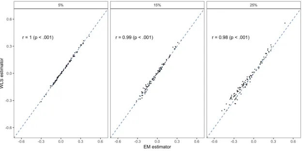
Figure 4: EM and WLS estimators of the bias term are highly correlated.
Next we estimate V ar(ˆδEM). Since the likelihood function is not a regular likelihood and