DATA MINING cDNA MICROARRAY EXPERIMENT WITH A
GEE APPROACH
MENG WU
A Thesis Submitted to the
University of North Carolina at Wilmington in Partial Fulfillment Of the Requirements for the Degree of
Master of Arts
Department of Mathematics and Statistics University of North Carolina at Wilmington
2004
Approved by
Advisory Committee
Chair
TABLE OF CONTENTS
ABSTRACT . . . iii
DEDICATION . . . iv
ACKNOWLEDGMENTS . . . v
LIST OF TABLES . . . vi
LIST OF FIGURES . . . vii
1 INTRODUCTION . . . 1
2 BACKGROUND . . . 2
2.1 cDNA Microarray . . . 2
2.2 Experiment and Data . . . 3
2.3 Normalization . . . 5
3 GENERALIZED ESTIMATING EQUATION . . . 13
3.1 Theory and Motivation . . . 13
3.1.1 Generalized Linear Model . . . 13
3.1.2 GEE . . . 15
3.2 Model . . . 17
4 FALSE DISCOVERY RATE . . . 19
4.1 Definition . . . 19
4.2 Q-values . . . 19
5 RESULTS AND CONCLUSION . . . 23
5.1 Results from Q-values . . . 23
5.2 Results from Multtest . . . 27
5.3 Conclusion . . . 28
REFERENCES . . . 31
APPENDIX . . . 33
SASr Program for GEE . . . 33
ABSTRACT
The use of microarray technology provides access to the simultaneous expression of thousands of genes and is revolutionizing the scientific community of functional genomics. This thesis investigates a cDNA microarray experiment with the goal of discovering differentially expressed genes across several factors. The analysis first ”normalizes” the data through the VSN package which is a robust calibration and variance stabilization software that removes systematic bias which could impair the analysis. A generalized estimating equation (GEE) approach is used to model the data and investigate the null hypothesis of no difference in expression levels. To accommodate the numerous hypothesis being tested, we used the q-value method to control the false discovery rate of the analysis. The analytical procedures are performed by using the statistical software packagesSASr and R.
DEDICATION
This thesis is dedicated to my grandma, WenJun Lu. She’s right now fighting bronchial disease and couldn’t be here, but her love and encouragement have inspired me all along.
ACKNOWLEDGMENTS
First and most of all, I would like to thank my advisor, Dr. Susan Simmons, for her great insight, guidance, patience, encouragement and being there for me every step of the way. This could not have been possible without her. I would also like to thank Dr. James Blum, for providing the data and helping me withSASr pro-gramming. I am also very grateful to Dr. Ann Stapleton for providing information regarding to her experiment and helping me with biological concept and terminology that I came across during my study. And I would like to thank Dr. James Blum and Dr. Dargan Frierson for reviewing my draft and willing to be in my advisory committee.
I would also like to express my sincere gratitude to all the faculty members and fellow students in the Department of Mathematics and Statistics for sharing their love and knowledge of mathematics and statistics with me.
LIST OF TABLES
LIST OF FIGURES
1 Histograms for all B73 arrays before normalization . . . 6
2 Histograms for all Mo17 arrays before normalization . . . 6
3 Histograms for all B73 after normalization . . . 7
4 Histograms for all Mo17 after normalization . . . 7
5 Before the variance stabilization and calibration procedure. . . 8
6 After the variance stabilization and calibration procedure. . . 9
7 Variance stabilization. . . 10
8 Q-value plots for treatment using software-pickedλ . . . 25
9 Q-value plots for treatment . . . 25
10 Q-value plots for line . . . 26
11 Q-value plots for interaction . . . 26
1 INTRODUCTION
The use of microarray technology provides access to the simultaneous expression of thousands of genes and is revolutionizing the scientific community of functional genomics. This technology generates high-dimensional complex data that represents the concurrent behavior of thousands of genes across various treatments, time points and/or applications [1]. The introduction of computationally intensive data anal-ysis methods has helped researchers deal with the huge amount of data produced by these experiments. Two common approaches of analyzing gene expression array data are the grouping of similarly expressed genes (i.e. cluster analysis), and the identification of statistically significant genes whose expression are changing under varying conditions. For the latter, the biological question of differential expression can be restated as a problem in multiple hypothesis testing; that is, the simultaneous test for each gene under the null hypothesis of no association between the expression levels and the responses or covariates [2].
Herein, a cDNA microarray experiment is analyzed with the goal of discover-ing differentially expressed genes across several factors. Inherent in the experiment are statistical challenges that will be addressed in this thesis. The experimental design, along with the issues and goals of the analysis, are introduced in Chapter 2. Also included in this Chapter is an important process called normalization that removes systematic bias that could impair the analysis. In Chapter 3, a generalized estimating equation (GEE) approach is used to model the data and investigate the null hypothesis of no difference in expression levels across the factors. To control the false discovery rate of the analysis, the q-value method is discussed in Chapter 4 with the results and conclusions in Chapter 5.
2 BACKGROUND
2.1 cDNA Microarray
The first step in the production of a microarray is the selection of the probes to be placed on the glass slide. Once the probes have been selected, they are amplified by a technique known as polymerase chain reaction (PCR) [3], and are placed on the cDNA microarray in approximately equal amounts by a high-speed robot. Each spot on the microarray corresponds to a gene or an EST (expressed sequence tag).
The investigators then extract total RNA or mRNA produced from the bio-logical sample. This may involve various cell types; for example healthy and tumor cells or treatment and control cells. By using reverse transcription, the mRNA from the two samples is fluorescently labelled with Cy3 (green) and Cy5 (red), and the target mixture is hybridized to the probes on the glass slides. The segments of the mRNA in the target and their complimentary portion among the samples of cDNA on the glass slide will bind together if finding each other during hybridization. When completed, the glass slide is washed and a luminous emission is measured by a scan-ning microscope. Fluorescent intensity for the red and green dye of each spot is measured separately, and provides a measure of the relative mRNA abundance for each gene expression in the two cells. The intensity of the green spot measures the relative mRNA abundance labelled with Cy3, while the intensity of the red spot measures the relative mRNA abundance labelled with Cy5. Gray spots represent genes that were expressed in neither cell type.
These measurements provide information about the relative level of expres-sion of each gene in the two cells. The monochrome images can be colored to provide
The two major types of microarrays are the spotted cDNA microarrays [4] and oligonucleotide arrays [5]. The genomic material used to make the array, the manner in which this material is actually placed on the array, and the design of the experiments are the defining differences between these two methodologies. Typically, oligonucleotide arrays are based on the total genome sequence of a particular organ-ism, and uses strings of oligonucleotide as the probes. Another interesting factor of the oligonucleotide array is that every probe, referred to as PM (perfect match), is paired with a single homomeric base change (A ↔T, G ↔ C) probe referred to as MM (mismatch) [1]. This mismatch probe is designed to be a hybridization control for the PM probe. The assessment of every gene in an organism under certain sce-narios, when compared to a control, provides a subset of genes that are responding to a stimulus, and thus reacting in the genome.
2.2 Experiment and Data
The experiment is designed to find differentially expressed genes between UV treatment and control in two inbred lines that are the foundation for many mapping studies in maize (Dr. Stapleton, personal communication). The design emphasizes the detection of UV specific effects and interactions between UV exposure and line. In the experiment, individual seeds were placed one per 6 cm pot, at a density of 36 pots per flat, and grown in the greenhouse without supplementary lighting for ten days to the two-leaf stage. The two lines were then exposed to 4 hours of ultravio-let radiation from UV313 bulbs suspended about 30 cm above the plants. Control plants were placed under UV313 bulbs covered with polyester, which transmits visi-ble light but excludes UV-B. After UV irradiation, the UV bulbs were turned off and the plants were allowed to recover for 4 hours in the greenhouse. The second and
third seedling leaf from each of four plants were harvested and dropped immediately into liquid nitrogen. Total RNA was extracted from frozen tissue, and the cDNA samples were labeled using Cy5 or Cy3, with excess nucleotide and primers removed via PCR purification kit.
The experiment involved eight maize cDNA Unigene slides, four slides for the B73 line and four slides for the Mo17 line. Within these cDNA microarrays, the genetic material is printed three times next to each other; consequently, average signal intensities and ratio between co-hybridized samples could be assessed multi-ple times within each microarray and within experiments. The four arrays within each line set contained duplicate dye swaps for the UV-B treatment and control. In these dye swapping experiments, the RNA samples from different experiments were labelled reciprocally.
The data from this experiment was graciously obtained from Dr. James Blum in a SAS data set with eight columns and a total of 270,512 observations. The columns in this data set are as follows:
Column 1 – id, the biological description of each gene
Column 2 – name, the gene names as referenced in the experiment Column 3 – spot, the location of the spot on the array
Column 4 – intensity, expression levels for the corresponding gene Column 5 – array, the array to which the spot belongs. Levels: 1,2,3,4.
Column 6 – dye, color of dye used for the corresponding gene. Levels: green, red.
Column 7 – line, line information. Levels: B, M.
2.3 Normalization
Due to the many sources of variation inherent in a microarray experiment, it is important that we remove any systematic variation detected. Even in the replicate arrays variations are commonly observed. The purpose of normalization is to adjust for effects which arise from variation in the microarray technology rather than from biological differences. These variations may arise due to imbalances between red and green dyes caused by labelling efficiencies or scanning properties. Other sources of variation include the location of the spot which may include some spatial vari-ation, or variation due to print-tip; and other differences in print quality, ambient conditions or simply the scanner settings. Therefore normalization between as well as within arrays will need to be considered.
We utilized the VSN software developed by Huber [9], in the bioconductor project (www.bioconductor.org) to normalize the data. The VSN software is a ro-bust calibration and variance stabilization tool, that removes the dependency of the variance on the mean. The VSN package provides a calibration procedure and trans-formation of the expression levels in one model with parameters estimated from the data. The calibration procedure uses an affine-linear mapping to bring the various samples onto the same scale, and then performs an arcsinh transformation on the data. The normalized data should have mean expression levels that are independent of the variance and on a consistent scale.
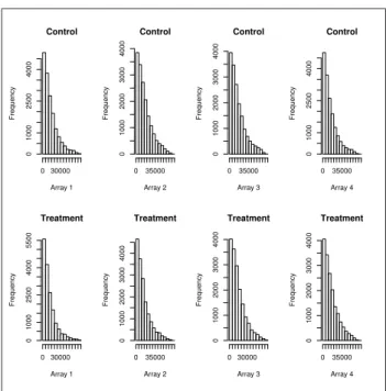
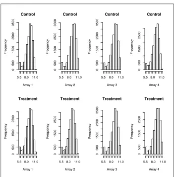
Figures 1-4 give histograms of the gene expression level distributions before and after normalization. The top rows of each figure depict distributions of the four controls used on the arrays, while the bottom rows depict distributions of the four UV-B treatments used on arrays. We can see that before normalization the
distri-Control Array 1 Frequency 0 30000 0 1000 2500 4000 Control Array 2 Frequency 0 35000 0 1000 2000 3000 4000 Control Array 3 Frequency 0 35000 0 1000 2000 3000 4000 Control Array 4 Frequency 0 35000 0 1000 2500 4000 Treatment Array 1 Frequency 0 30000 0 1000 2500 4000 5500 Treatment Array 2 Frequency 0 35000 0 1000 2000 3000 4000 Treatment Array 3 Frequency 0 30000 0 1000 2000 3000 4000 Treatment Array 4 Frequency 0 35000 0 1000 2000 3000 4000
Figure 1: Histograms for all B73 arrays before normalization
Control Array 1 Frequency 0 30000 0 2000 4000 6000 Control Array 2 Frequency 0 30000 0 1000 3000 5000 Control Array 3 Frequency 0 30000 0 2000 5000 8000 Control Array 4 Frequency 0 30000 0 2000 5000 8000 Treatment Array 1 Frequency 0 30000 0 2000 4000 6000 8000 Treatment Array 2 Frequency 0 30000 0 2000 4000 6000 Treatment Array 3 Frequency 0 30000 0 2000 4000 6000 Treatment Array 4 Frequency 0 30000 0 2000 4000 6000
Control Array 1 Frequency 5.5 8.0 11.0 0 500 1500 2500 3500 Control Array 2 Frequency 5.5 8.0 11.0 0 500 1500 2500 3500 Control Array 3 Frequency 5.5 8.0 11.0 0 500 1500 2500 3500 Control Array 4 Frequency 5.5 8.0 11.0 0 500 1500 2500 Treatment Array 1 Frequency 5.5 8.0 11.0 0 500 1500 2500 Treatment Array 2 Frequency 5.5 8.0 11.0 0 500 1500 2500 Treatment Array 3 Frequency 5.5 8.0 11.0 0 500 1500 2500 3500 Treatment Array 4 Frequency 5.5 8.0 11.0 0 500 1500 2500
Figure 3: Histograms for all B73 after normalization
Control Array 1 Frequency 5.5 8.0 11.0 0 500 1500 2500 3500 Control Array 2 Frequency 5.5 8.0 11.0 0 500 1500 2500 3500 Control Array 3 Frequency 5.5 8.0 11.0 0 500 1500 2500 3500 Control Array 4 Frequency 5.5 8.0 11.0 0 500 1500 2500 Treatment Array 1 Frequency 5.5 8.0 11.0 0 500 1500 2500 Treatment Array 2 Frequency 5.5 8.0 11.0 0 500 1500 2500 Treatment Array 3 Frequency 5.5 8.0 11.0 0 500 1500 2500 3500 Treatment Array 4 Frequency 5.5 8.0 11.0 0 500 1500 2500
butions of both lines have a fair amount of skewness, while after the procedure the lines exhibit a more stable distribution that is more symmetric in nature.
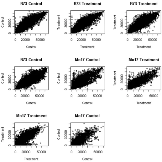
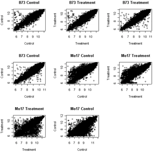
Figure 5 illustrates the raw expression levels when we compare duplicate ar-rays. For example, the first graph depicts the relationship between the control on array 1 and the control on array 2. These two arrays are duplicates in the sense that they are subjected to identical experimental conditions and the treatment/control groups are labeled the same.
Figure 6 illustrates the same arrays after normalization via the VSN pack-age. Generally, all plots have similar shape and range, which indicates the systematic array- or dye-biases appear to have been removed. By looking at the plots, it appears that the normalization procedure performed better on the B73 line. The majority of data points from these 4 B73 plots are well clustered about a diagonal line, while those from Mo17 line, although improved, still have a considerable amount of noise. This is most likely caused from the extreme skewness in the Mo17 line. Both lines exhibit skewness; however, it is much more prominent in the Mo17 line. This prop-erty proved to be relatively difficult to deal with by this or similar normalization methods, and needs further investigation.
As shown in Figure 7, we can see that after transformation the variance is stabilized successfully. The big black dots, connected by lines, show the running median of the standard deviation. The curve given by the connected line is an es-timate of the systematic dependence of the standard deviation on the mean. We can see after variance stabilization, it is an approximately horizontal line without much overall trend, which indicates that the variance is approximately independent of the mean intensity. The overall procedure appears to have worked well; however,
we notice that at the lower end of the rank of the mean, standard deviations are unusually spread out. Of course ideally we want the majority of the standard devi-ation clustered at lower values.
3 GENERALIZED ESTIMATING EQUATION
3.1 Theory and Motivation
The assumption of normality for data produced in a microarray experiment is not necessarily a valid one. Also the cDNA microarray under investigation consists of three replicated spots for each gene sequence, which induces a correlation among these spots. This correlation must be taken into account for proper inference and valid hypothesis testing, which is why a GEE model with quasi-likelihood estimators was chosen for this analysis.
GEE, Generalized Estimating Equations, was first proposed by Liang and Zeger [6] as a modelling strategy for correlated and clustered data. It is an ex-tension of Generalized Least Squares approach [7] to non-Normal distributions by introducing quasi-likelihood methods that can manage correlation structure found in panel data and longitudinal or repeated measures analysis.
3.1.1 Generalized Linear Model
A generalized linear model has 3 components: the linear predictor, the link function, and the distribution of the response variable [8]. The Linear Predictor, which we will denote by η, is η = Xβ, where the parameters β enter in a linear fashion. The link function is a function of the mean that links the distribution of the response to the linear predictor. If we denote the mean ofyasE(y) = µ, then the link function can be represented as g(µ), where g(µ) = Xβ, or µ= g−1
(Xβ). The third component of a generalized linear model is the distribution of the response variable, which is assumed to belong to the exponential family of distributions.
Members of the exponential family of distributions can be written as:
f(y) = exp{yθ−c(θ)
a(φ) +h(y, φ)} (1)
whereθ is known as the canonical parameter and is a function of µ, andφ is known as a ”dispersion” or ”scale” parameter.
For example, in the Normal distribution,
f(y) = √ 1 2πσ2 exp(− (y−µ)2 2σ2 ) = exp[−y 2 −2yµ+µ2 2σ2 − 1 2ln[2πσ 2 ]] = exp{yµ− µ2 2 σ2 −[ y2 2σ2 + 1 2ln(2πσ 2 )]} where θ = µ c(θ) = µ 2 2 a(φ) = σ2 h(y, φ) = −1 2[ y2 σ2 + ln(2πσ 2 )]
The estimating equation in a likelihood based model is the first derivative of the log likelihood, otherwise known as the score function. In case of the exponential family, the score function can be derived by the use of chain rule where,
∂l ∂β = ∂l ∂θ ∂θ ∂µ ∂µ ∂η ∂η ∂β
In the case of the exponential family, this simplifies to:
∂l ∂βk =X i 1 V(µi)a(φ)[yi−µi] ∂µi ∂ηi xik (2)
where i = 1, . . . , n (n is the number of observations) and V(µi) specifies the relationship between the mean of yi and the variance of yi.
3.1.2 GEE
If one does not want to make an assumption regarding the probability function of
y, but instead make an assumption with respect to association between the mean and the variance, then likelihood methods should be employed. In the quasi-likelihood framework, the estimating equations are similar to the score function in the exponential family:
X i V−1 (yi−µi) ∂µi ∂β (3)
or, in matrix form D0
V−1 (y−µ) where V =V(µi)τ2 and D0 represents [∂µ∂β] or D0 = ∂µ1 ∂β1 · · · ∂µN ∂β1 ... ... ... ∂µ1 ∂βN · · · ∂µN ∂βN
In the situation where the observations are independent, the matrix V is diagonal matrix. However, in the case of correlated or ”panel” data, an approach is needed to incorporate this information. The seminal paper by Liang and Zeger [6] contributed a workable system for representing these ideas into the matrix V and a coherent estimation and interpretation strategy.
They derived a ”working correlation” matrix defined by R(α). In this con-text, we redefine the matrix V as follows:
V =A12R(α)A
1
2 (4)
whereR(α) is a n×nmatrix of correlation coefficients, numbers between−1 and +1, and is fully specified by the parameterα, andAi is a diagonal matrix with
V(µ) on the diagonal. A= V(µ1) 0 0 0 0 0 V(µ2) 0 0 0 0 0 . .. 0 0 0 0 0 V(µn−1) 0 0 0 0 0 V(µn)
Examples of some of the correlation matrices are:
Unstructured: 1 α12 · · · α1n α21 1 · · · α2n ... ... ... α3n αn1 αn2 · · · 1
αij, for each i6=j and i < j. Exchangeable: 1 α · · · α α 1 . . . α ... ... ... α α α · · · 1
The exchangeable correlation matrix assumes each correlation value,αij(i6=
j), is the same. Autoregressive (1): 1 α α2 · · · αn−1 α 1 α · · · αn−2 ... ... . .. ... αn−1 αn−2 · · · α 1
The autoregressive(1) correlation matrix assumes that observations closer to-gether are more similar than those farther apart.
The ”general estimating equations” are the result of taking this structure into account within a quasi-likelihood context. Thus, the estimating equations in the GEE paradigm are defined in equation (3) with theV matrix defined in equation (4). With these estimating equations, optimization programs, such as Newton-Raphson are used to estimate the parameters.
3.2 Model
We used the GENMOD procedure in SAS to fit a GEE model on a gene by gene basis to the normalized data. The experiment was treated as a split plot design with the ”block” (or array) considered as the ”whole plot”. For this analysis, we
as-sumed there was no array × treatment interaction. The validity of this assumption is an area of further investigation and is not considered in this thesis. The program code for this model is shown in Appendix 1. The first model includes terms for line, treatment, dye and line × treatment interaction. The second model removes the the line × treatment interaction for those genes who did not have a significant the line× treatment interaction. The p-values for the line × treatment interaction were recorded after the first model, and the p-values for the line and treatment were recorded after the second model.
In the GENMOD procedure, the specified covariance structure of the GEE model is based on eight clusters (panels), or the eight arrays in the experiment. We assumed the correlation coefficients consistent across observations, therefore chose the Exchangeable Correlation Matrix as the structure for the correlation matrices.
4 FALSE DISCOVERY RATE
4.1 Definition
Classical multiple comparison procedures aim at controlling the probability of committing even a single type-I error within the tested family of hypotheses. The main problem with such classical procedures, is that they tend to have substantially less power than uncorrected procedures. In many instances, lack of multiplicity con-trol is too permissive, but the full protection resulting from concon-trolling the Family-wise Error Rate (FWER) is too restrictive. Benjamini and Hochberg [10] introduced the False Discovery Rate (FDR) - the expected ratio of erroneous rejections to the number of rejected hypotheses, as an appropriate error rate to control. The FDR is equal to the family wise error rate when the number of true null hypotheses m0
equals the number of all hypotheses being tested (m) [12], so in such a situation controlling the FDR controls the FWER as well. But the FDR criterion is adaptive, in the sense that when some of the tested hypotheses are not true (i.e. m0 < m), the
FDR is smaller, and more so when more of the hypotheses are not true. Hence FDR controlling procedures can be more powerful than FWER controlling procedures at the same level.
4.2 Q-values
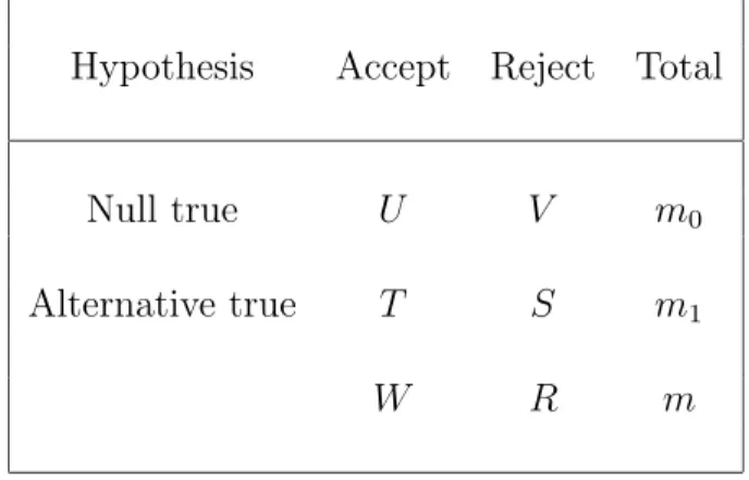
Table 1 [12] describes the possible outcomes in testingm hypotheses. Note that
R is the total number of hypotheses rejected, and V is the number of false positive results. So FWER, which is the probability of making one or more type I errors among all the hypotheses, is defined to be Pr (V ≥ 1). As a very strict error measure, when the number of tests increases, the power in the FWER procedure decreases [11]. On the other hand, FDR is defined to be the expected proportion of
Table 1: Outcomes when testing m hypotheses
Hypothesis Accept Reject Total
Null true U V m0
Alternative true T S m1
false positive findings among all rejected hypotheses times the probability of making at least one rejection.
F DR =E[V
R|R >0]P r(R >0) (5)
Benjamini and Hochberg [10] provided sequential p-value methods to fix the error rate beforehand and to estimate the rejection region.
Storey [12] introduced the positive False Discovery Rate (pFDR), defined as:
pF DR=E[V
R|R >0] (6)
The additional term ”positive” refers to the fact this quantity is estimating an error rate where at least one positive finding has occurred.
In a multiple hypotheses setting, test statistics for each of them hypotheses are calculated, T1, T2,· · ·, Tm and each null hypothesis will either be regarded as true, H = 0, or false H = 1. If we define the rejection region for these hypotheses test asθ, and the probability that a null hypothesis is true witha priori probability
pF DR = π0P(T ∈θ|H = 0)
π0P(T ∈θ|H = 0) +π1P(T ∈θ|H = 1)
(7)
where π1 = 1−π0
An estimate of π0 can be obtained by
c
π0(λ) =
](Pi > λ)
(1−λ)m (8)
for some λ, where Pi is the p-value for hypothesis i.
The q-value, defined by John Storey [11], is the minimum pFDR at which a gene can be called differentially expressed, and is defined as:
q−value(t) = inf
t∈θP r(H = 0|T ∈θ) (9) This q-value corresponds to the posterior probability that a gene is not def-erentially expressed given that gene statistic is as extreme as the one observed for this gene in the data. These q-values may be used by the investigator as criteria for selecting all features with q-value less or equal to a chosen false discovery rate threshold value. We utilized John Storey’s Q-value software in R for our analysis.
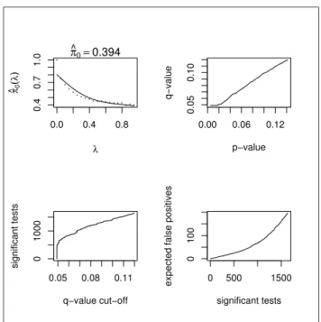
Storey [11] provides four useful plots through his Q-value software. Through these plots, an investigator can choose the optimal q-value or p-value for the analy-sis. The plots produced in the Q-value software are:
1. The estimatedπ0 versus the tuning parameter λ
2. The q-values versus the p-values
3. The number of significant tests versus each q-value cut-off
5 RESULTS AND CONCLUSION
5.1 Results from Q-values
Storey [12] recommends allowing the Q-value software to estimate the optimalλ
for the analysis. The software estimates theM SE forλ values ranging from 0.00 to 0.95, and chooses the value that minimizes the M SE. The value for λ is then used to estimate π0, which is the a priori P(H = 0). However, using this approach to
estimate λ for our data gives unreliable results. For example, using the p-values of the treatment effect and the estimate ofλ provided by the software, π0 is estimated
to be 0.39 indicating that the majority of the genes are believed to be significant, or differentially expressed, which is very unlikely. Also, the second plot in Figure 8 shows that for a p-value of 0.05 the corresponding q-value is approximately the same, and a p-value of 0.1 yields a q-value less than 0.1. Since p-values measure the error rate of a individual test while q-values measure the overall error rate, it does not make sense to have q-values less than or equal to the corresponding p-values. Therefore, we decided to choose aλ that produces reasonable value of π0 and make
the analysis more appropriate. We calculated an estimate of π0 from the data by
calculating the proportion of p-values≤0.05. By using this estimate ofπ0, we were
able to calculate more appropriate values of λ that yielded more consistent results.
The estimate ofλfor the treatment p-values was estimated to be 0.065, with
π0 = 0.715. The resulting graphs from the Q-value software are shown in Figure 9.
Again we use a p-value cut-off of 0.05, which yields a q-value of about 0.12. Thus, we expect approximately 1014 significant tests, among which there are about 120 false positives.
The estimate of λ for the line p-values was estimated to be 0.06, with
π0 = 0.762. The graphs for this analysis are shown in Figure 10. With the same
cut-off p-value of 0.05, the corresponding q-value is around 0.155. Thus, we expect approximately 851 tests to be significant, among which there are about 132 false positives.
The estimate ofλfor the interaction p-values was 0.1, which gave an estimate of 0.918 for π0. Figure 11 illustrates the q-value results of this analysis. According
to this output, if we select a p-value of 0.05 as our cut-off, the q-value, or pFDR is around 0.48. We feel that 48% is rather high for a false discovery rate and conclude there were no significant interactions.
0.0 0.4 0.8 0.4 0.7 1.0 λ π ^(λ0 ) π ^0=0.394 0.00 0.06 0.12 0.05 0.10 p−value q−value 0.05 0.08 0.11 0 1000 q−value cut−off significant tests 0 500 1500 0 100 significant tests
expected false positives
Figure 8: Q-value plots for treatment using software-picked λ
0.0 0.4 0.8 0.4 0.7 1.0 λ π ^(λ0 ) π ^0=0.715 0.00 0.10 0.10 0.20 p−value q−value 0.10 0.20 0 1000 q−value cut−off significant tests 0 500 1500 0 200 significant tests
expected false positives
0.0 0.4 0.8 0.0 0.6 λ π ^(λ0 ) π ^0=0.762 0.00 0.05 0.10 0.15 0.16 0.19 p−value q−value 0.16 0.18 0.20 0 1000 q−value cut−off significant tests 0 500 1500 0 200 significant tests
expected false positives
Figure 10: Q-value plots for line
0.0 0.4 0.8 0.6 0.9 λ π ^(λ0 ) π ^0=0.918 0.05 0.20 0.35 0.48 0.56 p−value q−value 0.48 0.54 0.60 0 2000 q−value cut−off significant tests 0 1000 2500 0 1000 significant tests
expected false positives
5.2 Results from Multtest
The biological question of differential expression can be viewed from a multiple hypothesis perspective: the simultaneous test for each gene of the null hypothesis of no association between the expression levels. We attempt to compare the results obtained from the GEE approach and Q-value method to those provided through a packaged multiple comparison procedure developed by Dudoit et al. [13].
Themulttestpackage under the Bioconductor project was developed in R by
Dudoit and Ge [13]. It performs different procedures such as t-test, F-test, paired
t-test, block F-test and Wilcoxon test that produce p-values which can be adjusted to control the family wise Type I error rate (FWER). Some of the procedures used to adjust p-values are Bonferroni, Hochberg, Holm, Sidak, Westfall, Minp and MaxP etc. [13].
Standardized intensities for both Mo17 and B73 lines were analyzed with the
multtestpackage separately. The results show that all the adjusted p-values for each
gene are calculated to be 1, therefore fail to choose any significant genes. Due to the inconsistency between this and our previous results, we decided to run the data through the Significance Analysis of Microarray (SAM) to take another look at a different multiple testing procedure. A basic SAM analysis was conducted for the normalized intensities for each line separately, with 500 balanced permutations. The results from SAM procedure indicates no significant genes in either line. Since both
multtestandSAM only accept single measurement for each gene, we calculated the
average intensities as the response variable for both analysis. Analyzing the lines separately and only using the average intensity for each gene on an array reduces the number of observations per gene, which in turn reduces the power for detecting
differentially expressed genes.
5.3 Conclusion
The rich information provided by microarray experiment gives possibilities to discover gene expression patterns under various treatments and/or factors. Design of the experiment always plays an important role in the analysis of the data. Differ-ent analysis methodologies however, may yield differDiffer-ent results. The question as to which method is best is still an open question.
We chose Generalized Estimating Equations for this correlated (3 replicated spots) and clustered (8 arrays) data to ensure proper inference for the layout of the experiment. Among the 5,376 genes, 1,014 genes are found to be significant (with 140 expected false positives) for the treatment effect. We infer that those genes are possibly related to the UV treatment and remain as potential candidates for future biological study. We also found 851 out of 5,376 genes significant (with 132 expected false positives) for the line factor indicting that these genes have possible significant different expression levels between the two lines, and should be subjected to future biological study. We conclude no significant genes for the line× treatment interac-tion due to high false discovery rates. This means that the UV-B treatment affects the expression levels similarly within each line.
The box plots in Figure 12 illustrate that treatment and control for both lines have very similar distributions (from left to right, the box plots are: treatment for Mo17, control for Mo17, treatment for B73, control for B73). GEE method treats the data as a whole while multtest and SAM analyze Mo17 and B73 lines
5.5 6.0 6.5 7.0 7.5 8.0 8.5 9.0 9.5 10.0 10.5 11.0 5.5 6.0 6.5 7.0 7.5 8.0 8.5 9.0 9.5 10.0 10.5 11.0 6 7 8 9 10 11 6 7 8 9 10 11 12 Figure 12: Bo x plots for treatmen t and con trol on b oth lines 29
of bothmulttest and SAM to pick up any significant genes is an interesting discov-ery. Because of the significant sample size reduction for both packages (only 1/6 of the sample size of the GEE analysis), one may argue that a comparison could be inappropriate. However, considering the rather large difference between the results (1014 significant genes versus 0), we still feel that although contributed by its larger sample size, the GEE method appears to have more power in detecting differentially expressed genes for UV-B treatment versus a control. However it is unclear as to which method is the optimal for this analysis.
Although the analysis provides reasonable results, a few issues remain unre-solved. A better normalization procedure, validation of the assumption of no array × treatment interaction and what method is the optimal method to use have not been considered in this thesis and are still open areas for future investigation.
REFERENCES
[1] B.A. Craig, M.A. Black and R.W. Doerge “Gene Expression Data”, Journals of Agricultural, Biological, and Enviromental Statistics, Volumn 8, Number 1, Pages 1-28, 2003.
[2] Sandrine Dudoit, Juliet Propper Shaffer and Jennifer C. Boldrick, “Multiple Hypothesis Testing in Microarray Experiments” Statistical Science, Vol 18, No. 1, 71-103, 2003.
[3] Paola Sebastiani, Emanuela Gussoni, Isaac S.Kohane and Marco F.Ramoni, “Statistical Challenges in Functional Genomics”, Statistical Science, Vol. 18, No.1, 33-70, 2003.
[4] Schena M., Shalon D., Davis R. W., aand Brown P. O., “Quantitative Moni-toring of Gene Expression Patterns with a Complementary DNA Microarray”,
Science, 270, Page 467-470, 1995.
[5] Lockhart DJ, Dong H, Byrne MC, Follettie MT, Gallo MV, Chee MS, Mittmann M, Wang C, Kobayashi M, Horton H, Brown EL., “Expression monitoring by hybridization to high-density oligonucleotide arrays”,Nature Biotechnology, 14, Page 1675-1680, 1996.
[6] Liang, K.-Y. and Zeger, S. L., “Longitudinal data analysis using generalized linear models”,Biometrika, 73, 13-22, 1986.
[7] Greene, W. H., Econometric Analysis, 2 edn, Mac Millan, New York, 1993.
[8] McCullagh, P. and Nelder, J. A., Generalized Linear Models, Chapmann and Hall, London, 1989.
[9] W. Huber, “Robust calibration and variance stabilization with VSN”, vignette in bioconductor project, www.bioconductor.org, October, 2003.
[10] Benjamini, Y. and Hochberg, Y., “Controlling the false discovery rate: A prac-tical and powerful approach to multiple testing”Journal of the Royal Statistical Society, Series B 85: 289300, 1995.
[11] Storey JD., “The positive false discovery rate: A Bayesian interpretation and the q-value”Annals of Statistics, Vol 31: 2013-2035, 2003.
[12] Storey JD., “A direct approach to false discovery rates” Journal of the Royal Statistical Society, Series B, 64: 479-498, 2002.
[13] Sandrine Dudoit and Yongchao Ge, “Bioconductor’s multtest package”, vi-gnette in bioconductor project, www.bioconductor.org, May, 2004.
APPENDIX
SAS Program for GEE
MODEL 1 proc genmod data = test;
class dye array line treatment;
model intensity = line dye treatment line*treatment/dist=normal type3; repeated subject=array/type=exch;
lsmeans line*treatment; by name;
make ’type3’ out=p_table; make ’lsmeans’ out=lsmeans; run;
data p_value; set p_table;
if source=’line*treatment’ then p_value=ProbChiSq;
if mod(_N_,4)=0 then output; keep name p_value;
MODEL 2
proc genmod data = test2; class dye array line treatment; model intensity = line dye treatment/dist=normal type3;
repeated subject=array/type=exch; by name;
make ’type3’ out=p_table; run;
data p_value_line; set p_table;
if source=’line’ then p_value=ProbChiSq;
if source=’treatment’ then delete; if source=’dye’ then delete;
keep name p_value; run;
data p_value_trt; set p_table;
if source=’line’ then delete;
if source=’treatment’ then p_value=ProbChiSq; if source=’dye’ then delete;
keep name p_value; run;