The Aquila Digital Community
The Aquila Digital Community
Dissertations
Spring 5-2010
Guppie: A Coordination Framework for Parallel Processing Using
Guppie: A Coordination Framework for Parallel Processing Using
Shared Memory Featuring A Master-Worker Relationship
Shared Memory Featuring A Master-Worker Relationship
Sean Christopher McCarthy
University of Southern Mississippi
Follow this and additional works at: https://aquila.usm.edu/dissertations Part of the Programming Languages and Compilers Commons
Recommended Citation Recommended Citation
McCarthy, Sean Christopher, "Guppie: A Coordination Framework for Parallel Processing Using Shared Memory Featuring A Master-Worker Relationship" (2010). Dissertations. 935.
https://aquila.usm.edu/dissertations/935
This Dissertation is brought to you for free and open access by The Aquila Digital Community. It has been accepted for inclusion in Dissertations by an authorized administrator of The Aquila Digital Community. For more
The University of Southern Mississippi
GUPPIE: A COORDINATION FRAMEWORK FOR PARALLEL PROCESSING USING SHARED MEMORY FEATURING A MASTER-WORKER RELATIONSHIP
by
Sean Christopher McCarthy
Abstract of a Dissertation Submitted to the Graduate School of The University of Southern Mississippi in Partial Fulfillment of the Requirements for the Degree of Doctor of Philosophy
ABSTRACT
GUPPIE: A COORDINATION FRAMEWORK FOR PARALLEL PROCESSING USING SHARED MEMORY FEATURING A MASTER-WORKER RELATIONSHIP
by Sean Christopher McCarthy May 2010
Most programs can be parallelized to some extent. The processing power available in computers today makes parallel computing more desirable and attainable than ever before. Many machines today have multiple processors or multiple processing cores making parallel computing more available locally, as well as over a network. In order for parallel applications to be written, they require a computing language, such as C++, and a coordination language (or library), such as Linda. This research involves the creation and implementation of a coordination framework, Guppie, which is easy to use, similar to Linda, but provides more efficiency when dealing with large amounts of messages and data. Greater efficiency can be achieved in coarse-grained parallel computing through the use of shared memory managed through a master-worker relationship.
COPYRIGHT BY
SEAN CHRISTOPHER MCCARTHY 2010
DEDICATION
To My Mother, Father, Grandfather, and Wife Kimberly
ACKNOWLEDGEMENTS
I would like to thank Dr. Ray Seyfarth and the other committee members, Dr. Joe Zhang, Dr. Louise Perkins, Dr. Andrew Strelzoff, and Dr. Jonathan Sun for their advice and support throughout this long process. I would especially like to thank Dr. Seyfarth. He has helped me tremendously and kept me motivated throughout my doctoral study. I would also like to thank Dr. Perkins for taking me under her wing after my senior level software engineering class. She has always believed in me, which in turn helped me to believe in myself.
I would also like to thank my family. My wife Kimberly has supported my decision to remain in school the entire time we have known each other. I would also like to thank my mother and father. I never would have been able to enroll in graduate school if it were not for them. They have helped to support me emotionally and financially all the way through.
I also want to take the time to acknowledge my grandfather. He died when I was very young, but it was his dream to one day have a doctor in the family. I know that he would be very proud of me if he were alive today.
TABLE OF CONTENTS
ABSTRACT ... ii
DEDICATION ... iii
ACKNOWLEDGEMENTS ... iv
LIST OF ILLUSTRATIONS ... vii
CHAPTER I. INTRODUCTION ... 1
II. COORDINATION LANGUAGES ... 4
Linda Linda’s Preprocessor III. LINDA EXTENSIONS ... 10
FT-Linda Bauhaus Linda Law-governed Linda LIME Extensions Review IV. OPENMP AND MPI ... 16
OpenMP MPI V. GUPPIE ... 30
Guppie’s Main Functions
Guppie Master Process Example Guppie Complete Example Templated Functionality Specialized Buffer
Guppie’s Shared Memory v
VI. GUPPIE’S SHARED MEMORY VS MPI’S
MESSAGE PASSING ... 51 Execution Times and Analysis
VII. CONCLUSION AND FUTURE WORK ... 65
APPENDIXES ... 68
REFERENCES ... 85
LIST OF ILLUSTRATIONS
Figure
4.1 OpenMP Array Example ... 22
4.2 MPI Hello World Example ... 24
4.3 MPI Send and Receive Functions ... 26
4.4 MPI Array Example ... 27
5.1 Master Starting Worker Processes in Guppie ... 34
5.2 Guppie Master Process ... 35
5.3 Guppie Worker Process ... 36
5.4 Guppie Templates ... 42
5.5 Guppie Buffer ... 45
5.6 Guppie Buffer Contents ... 46
6.1 Guppie Master Creating and Using Shared Memory ... 53
6.2 Guppie Worker Attaching and Using Shared Memory ... 55
6.3 Results (10 Averaging Iterations) ... 58
6.4 Results (1 Averaging Iteration) ... 61
CHAPTER 1
INTRODUCTION
Parallel computing consists of dividing a problem composed of independent sub-problems into multiple tasks that can be solved simultaneously. These independent tasks can be spread among multiple processors with each processor responsible for operating on its set of tasks. Once all processors have completed their tasks, the results are combined to form a solution to the original problem. Dividing an independent problem into multiple tasks, sending the tasks to multiple processors, performing a specific set of instructions by each processor on its tasks, and then combining the results of those instructions are the main steps in parallel computing.
Parallel processing can be achieved on either a local machine with multiple processors or over a network consisting of multiple machines. The machines connected by a network can either be multi-core or single-core. As long as there are multiple processors that can be used to solve a problem, and that problem can be divided into multiple tasks, parallel computing can be achieved.
The current trend in parallel computing is to use the processors in multiple machines connected by a network. This is referred to as distributed memory parallel processing. The computers used in distributed memory parallel processing might be in a dedicated cluster or even a collection of computers connected over the Internet. This is beneficial in that any machine with a processor (or multiple processors) can be added to the network to help parallelize a problem. The disadvantage to using multiple machines connected by a network is that there is added communication cost involved when sending
data from one process to another. This communication cost can be substantial when working with large data sets, such as images. For instance, sending an image containing one thousand rows and columns consists of sending one million pixels. Each pixel consists of red, green, and blue values, so the user is sending three million values from one process on one machine to another process on another machine. That is three million values that have to be sent and received by processes before computation is even started! There is another parallel computing paradigm to consider, and that paradigm is shared memory.
When multiple CPUs or multiple processor cores exist within a single machine, the user can take advantage of shared memory to help perform parallel computations. This is very advantageous when working with large data sets, such as images. By placing an image into shared memory, multiple processes can connect to the shared memory to retrieve the image, rather than having to send the entire image across a network to a process on another machine. The downside to this approach is that dedicated clusters can be built using thousands of processors while shared memory computers typically have fewer processors.
Both the shared memory and distributed memory parallel processing paradigms are analyzed in this dissertation. The two most popular parallel processing libraries, MPI and OpenMP, are discussed and compared to the Guppie parallel processing coordination framework developed as part of this research. Guppie utilizes shared memory features to reduce the need for communication and also provides a lot of the same features seen in the Linda coordination language. Like Linda, Guppie features a shared tuple space which is basically a shared associative memory system. In addition to the tuple space, Guppie
includes facilities for managing actual shared memory regions. By using Guppie’s shared memory features, along with its tuple space, it can be shown that Guppie is easier to use, and when working with large data sets, Guppie achieves better performance than its counterparts, MPI and OpenMP.
In the following two chapters, coordination languages are explained and
discussed. Then, the two most popular parallel processing libraries, OpenMP and MPI, are discussed. Guppie follows the OpenMP and MPI chapters. Then, a parallel image processing application written in both MPI and Guppie is compared, along with its CPU time, speedup, and efficiency results.
CHAPTER II
COORDINATION LANGUAGES
There are two major categories of parallel computing architectures which have been used in commercial systems: Single-Instruction Multiple-Data (SIMD) and
Multiple-Instruction Multiple-Data (MIMD) [34]. An example of a SIMD system is the Connection Machine 1 [50] which was popular for a brief period. The current trend in parallel computing is MIMD systems built using collections of microprocessor-based computers connected by networks.
A typical parallel application is built using both a computation and a coordination model1. A computation model can be a programming language, such as C++, Java, or Fortran. The computation model is used by programmers to build a serialized application in a computation language. A serialized application is a program that executes code one step at a time. Serialized code can be parallelized, at least to a certain degree, by
combining a coordination model with a computational model.
A coordination model coordinates how multiple processes function within the same application. The coordination model might be implemented as a library or as extensions to a language, forming a coordination language. MPI is an example of a coordination model implemented as a library [45]. OpenMP is a coordination model built with language extensions and a library [28]. Linda is an example of a coordination language [5,13,15,19].
1
It is possible to combine a computation model and a coordination model into a single language, but they are usually treated separately and combined together to form a parallel application. For example, the computation language C++ is its own stand-alone language, but it can be combined with a coordination language such as Linda or MPI to create a parallel application.
Linda
In order to understand how Guppie works, Linda should first be explained. Linda is a coordination model, and at its core is its tuple space [4,9,11,18,6]. A tuple is an ordered sequence of data, such as a string to represent a name, an integer to represent an identifier (id), and some values associated with that name and id. The tuple space is simply a collection of tuples. As well as creating the tuple space, Linda coordinates the way that processes interact with the tuple space.
Linda provides two different kinds of tuples, process tuples and data tuples. Process tuples are active, meaning that they can exchange data by generating, reading, and consuming data tuples. Data tuples are passive, and are the result of an executed process tuple. Another important feature of tuples is that they are atomic, meaning that a single attribute within an individual tuple cannot be modified unless the entire tuple is removed from the tuple space, modified, and placed back into the tuple space.
It is important to note that Linda is a distributed associative memory model, not a tool. There are many existing tools that implement the Linda memory model, such as implementations in Java [25,26] and C, such as CLinda [8,48]. Most implementations have the same set of Linda operations, so only CLinda, is described here. CLinda
provides functions to interact with the tuple space. CLinda has four main functions: out, in, rd, and eval.
out(t) causes tuple t to be added to the tuple space. The executing process
continues immediately. A tuple, as mentioned in the opening paragraph of this section, is a series of typed values, for example out("myData", 3.87, x, 5).
in(s) causes some tuple t that matches anti-tuple s to be withdrawn from the tuple space. An anti-tuple is some series of typed fields. These fields can either be actuals or formals. An actual is an actual field value, such as the string "myData" or the integer "3". Formals are place-holders for values that you are hoping to withdraw from the tuple that matches your actuals within the tuple space. A formal is prefixed with a question mark, for example ("myData", ?a, y, ?b) 2. Once in(s) has found a tuple t matching all the actuals in s, the values of the actuals in t are assigned to the corresponding formals in s, and the executing process continues. In the example t would match “myData” and y, while variables a and b would receive values from t. If no matching tuple t is available when in(s) executes, the executing process suspends until a matching tuple is available, and then the process proceeds as normal. If many matching tuples are available, then one is chosen arbitrarily.
rd(s) is the same as in(s) except that the matched tuple remains in the tuple space after rd(s) is executed.
eval(t) is the same as out(t) except that t is evaluated after, rather than before, it enters the tuple space. For example, suppose a user creates a function named
2
The use of the question mark, along with a few other syntactic issues, typically means that a special language processor is required in a Linda implementation.
“factorial(int)”, where an integer is passed as the parameter to the function, and the
function calculates the factorial of that parameter. The following eval function call eval(“fact”, 5, factorial(5)) places an active tuple into the tuple space. When the tuple
arrives in the tuple space, Linda creates a process to evaluate the function “factorial(5)”. Once evaluated, the computed value of “factorial(5)” replaces the function call in the
tuple, and the tuple becomes a passive data tuple.
There are also two predicate forms of the in and rd functions, inp and rdp. The only difference between these two forms is that they do not suspend if a matching tuple is not immediately available. inp and rdp return immediately with a true or false value.
Linda’s Preprocessor
Linda allows an arbitrary number of parameters in a tuple, and for input operations any of these parameters not preceded by a question mark are used for tuple selection. Versions of Linda have been developed for C for which a preprocessor is required to convert Linda operations into proper C syntax. There are several tasks that the Linda preprocessor must perform. The preprocessor must build a symbol table for determining variable types used in Linda operations, generate tuple usage information that may be used for load balancing, and modify the text of Linda calls for variable argument processing [1,2,10,12].
The Linda preprocessor has two phases. In the first phase, LPP-I, the
preprocessor expands all the C preprocessor directives, such as the #include header files. This is done in a single pass and then passed to a C compiler for error checking in the C part of the program. Once the errors are corrected, the input is ready for the second
phase, LPP-II. LPP-II checks for errors in Linda’s defined operators, such as in, out, rd, and eval. LPP-II then translates the code to the format needed by the kernel.
The C programming language has a preprocessor of its own, and Linda’s
preprocessor functions in a similar manner. The C preprocessor handles the directives for source file inclusion, such as the header files in the #include header statements found at the top of any C program. The preprocessor also handles #define macro definitions and
#if conditional inclusions. The preprocessor translates source code into an acceptable form for the compiler. Linda’s preprocessor performs similar operations in order for the
code to be compilation ready.
The preprocessor is also used to facilitate the run-time search. This is because Linda’s tuple space requires a great deal of searching for every Linda operation. One
responsibility of the Linda preprocessor is to match similar operators together based on the operator’s type of tuple space access. For example, the Linda operators “in” and “rd” are matched with “out” and “eval” and placed into groups based on matching tuple
patterns. Then, they are mapped onto the appropriate family of routines in the run-time library [17].
For C-Linda, the preprocessor is a C program that converts C-Linda programs into the syntax required by the C-Linda library. The preprocessor adds format strings containing type information to all Linda calls. This is achieved by scanning through the C-Linda program and tracking the types of variables and functions in their current contexts. There are some syntax modifications that need to be made as well. The Linda model uses the “?” operator for matching formals in the tuple space. The preprocessor
replaces each “?” with “&”. By replacing with an ampersand, a C compiler can pass the
formal parameter by reference and assign the correct value associated with the matching tuple into the memory space addressed by the formal parameter. Replacing the “?” operator with “&” is done for all parameters in Linda calls, except for parameters of
pointer types, such as strings and arrays. For these, the “?” operator is simply removed.
In order to compile C-Linda programs, a compiler interface must be used. A compiler interface is a C program that represents the C-Linda system in the form of a compiler. When a user wants to compile a C-Linda program, the compiler interface calls the preprocessor for every Linda source file, then produces the executable with the C compiler while linking with the C-Linda library.
CHAPTER III
LINDA EXTENSIONS
There are extensions of Linda's associate distributed memory model that solve problems encountered in Linda. FT-Linda [3] addresses issues with tolerating failures in the underlying computing platform. Bauhaus Linda [16,22] extends the Linda tuple space by having multiple tuple spaces in the form of multi-sets. Hybrid Law governed Linda [36] enforces a set of laws that all processes must follow in order to exchange tuples in the tuple space. Lime [29,44,46] utilizes mobile agents in their extension.
FT-Linda
One of Linda's shortcomings involves the inability to tolerate failures in the underlying computing platform. FT-Linda resolves this issue by providing stable tuple spaces and atomic execution of tuple space operations. Stable tuple spaces ensure that tuple values are not lost when failures occur. Atomic execution of tuple space operations allows tuple operations to be executed in an "all-or-nothing" manner, even despite
failures and concurrency.
Linda's lack of support for failures has an impact in two major ways. An application written using Linda cannot be recovered after an unexpected failure. If the execution time is short, then this may not be of much concern, but if the execution time is rather long, such as is needed for a decryption algorithm, the application may need to be restarted from the beginning. The other major impact of Linda's inability to tolerate
failures regards the near impossibility to write critical applications such as process control.
Fault tolerance in FT-Linda is achieved through the use of replication and
multicasting. Tuple spaces are replicated on multiple processors to ensure that data exists if a failure occurs, such as a processor failing. These tuple space copies are updated by use of an atomic multicast. This is an efficient implementation because only a single multicast message is needed for each collection of tuple space operations.
Bauhaus Linda
Bauhaus Linda is more powerful and simpler than the original Linda model. Bauhaus Linda simplifies Linda by combining similar features found in Linda into a single, collective feature. Bauhaus Linda generalizes Linda by not differentiating between tuples and tuple spaces, tuples and anti-tuples, or active (process) and passive (data) objects.
Tuples and tuple spaces are replaced by a single structure called a multiset. Normal Linda operations add (out), read (rd), and remove (in) tuples to and from a tuple space. Bauhaus uses the add, read, and remove functions to add or remove multisets to or from another multiset. This results in ordered tuples being replaced with unordered multisets.
In Bauhaus Linda a single tuple may function as a tuple space. Multiple elements may be added to or removed from a tuple. The opposite can be achieved as well. A tuple space may be treated like a single tuple. Bauhaus extends the out operation to allow tuple
space creation, just like it can create a tuple. The tuple space can then be manipulated as a single object. Since tuples and tuple spaces are treated as multisets, they acquire multiset operations such as union, intersection, and subtraction.
Bauhaus Linda does not differentiate between tuples and anti-tuples. Regarding Linda operations, out specifies a tuple, and in and rd specify an anti-tuple. Bauhaus is different in that all three operations take a multiset argument. The Bauhaus out operation adds a specified multiset to a target multiset, similar to how Linda would add a data tuple to a tuple space. However, since Bauhaus revolves around the use of multisets, Linda's type and position-sensitive associative matching rule is replaced by a simple set inclusion operation.
There is no distinction in Bauhaus Linda between active (process) and passive (data) objects. In Bauhaus, there is no need for an eval operation, as seen in the Linda model. Active and passive objects are still distinct in Bauhaus, but the way the
coordination language handles them is not. Bauhaus uses the out operation to handle both active and passive objects. Reading a process object in Bauhaus results in the reader's acquisition of a suspended copy of the process. Removing a process object in Bauhaus results in the remover's acquisition of the process itself, not a copy.
Law-Governed Linda
Linda's process communication with a tuple space is very efficient and easy. However, it is too simple, thus making communication unsafe. Law-governed Linda provides more secure process-tuple space interaction by providing additional attributes within tuples.
Law-governed Linda uses a concept already introduced in centralized and message passing systems. There are laws that processes must abide by in order to
communicate with the tuple space. These laws are needed because of Linda's inability to provide any security from eavesdropping or interference when a process must
communicate through a network to access a distributed shared memory tuple space that is common in the Linda model and the majority of its extensions. Linda gives processes the ability to read and remove tuples at will, even though some tuples may be intended to be received by particular processes. The message passing needed for processes to
communicate with a distributed shared memory tuple space assume that messages come from their apparent senders and are delivered to their intended recipients. However, this should not always be assumed due to problems in unrelated modules that could result in interference with a message.
Another problem regarding Linda's need for message passing is that it can be rather inefficient because it relies on an implicit convention, unknown to the Linda implementation. Linda's tuple space is usually distributed. The actual implementation, not the Linda model, is responsible for the placement and retrieval of tuples into the tuple space memory. The inefficiency is a result of the inability to determine the best
placement for a tuple. Obviously the best place for a tuple would be within or close to a processor that uses it most frequently, but this could be rather difficult to achieve. Global optimization of a distributed shared memory tuple space is feasible, but also impractical. The time needed to organize the tuples with processors that use them most frequently would create overhead that is comparable to the time needed to access them without being globally optimized.
LIME
LIME (Linda in a Mobile Environment) is a model that supports the development of applications that exhibit physical mobility of hosts, logical mobility of agents, or both. Linda uses a global, distributed shared memory, tuple space. Lime has mobile agents carry their own tuple spaces, which are shared between agents.
Tuple spaces are also extended with a notion of location, and programs are given the ability to react to specified states. The resulting model provides a minimalist set of abstractions that facilitate rapid and dependable development of mobile applications
Lime assumes that mobile agents exist in a set of hosts. These hosts are then connected through some network. Agents can then move from one host to another while carrying their tuple spaces with them. Access to the tuple space is performed using an extended set of tuple space operations. Each agent may own multiple tuple spaces, and these tuple spaces may be shared with other agents. Tuple spaces can be shared by extending the contents of each agent's local tuple space to include any tuples that exist in other agents' tuple spaces.
Extensions Review
One common feature found in the Linda model and its extensions is the focus on the tuple space being placed in distributed shared memory, meaning that the memory allocated for the tuple space can span over several computers. While the Lime model does not technically put the tuple space in distributed shared memory, it is still distributed amongst the mobile agents. Some processes or agents may even have local tuple spaces.
Tools invoking Linda's memory model might be implemented on top of a message
passing system like MPI. Data access control to the tuple space is also needed and can be achieved asynchronously through the use of a mutex or semaphore. When working with multiple computers using network communications, mutiple tuple server processes may be used as well. This involves defining a method for mapping tuples to servers so that there is a definite place to start searching for a tuple. There are more extensions than the ones listed above; however, none consider using shared memory to efficiently handle large data [38,39,41,42].
CHAPTER IV
OPENMP AND MPI
There are two main paradigms to consider for parallel computing. The first is shared memory multiprocessing (SMP). Historically SMP computers have been expensive computers with multiple processors sharing a single address space. Most of today's computers are multi-core computers, allowing shared memory parallel computing to be widely available. The other major paradigm is distributed memory parallel
computing. For this method, processors communicate with each over through a network. This method is utilized in systems ranging from small clusters using commodity network switches to supercomputers consisting of thousands of computers connected with
specially designed networks.
The main difference between the two paradigms is where the memory is stored. This effects how a parallel application is written. For shared memory parallel computing, different processes can access the same data. This is similar to referencing data in
serialized programs but adds the complexity of shared data integrity. Shared data integrity deals with read/write issues. For example, if multiple processes need to just read from the shared data, then there is no issue as long as no other process is currently trying to write to the data. If one process needs to update a value contained in a shared memory variable, the process needs to lock the shared memory variable so no other process has access to it. Once the process that is reading or writing to the shared memory has completed its operation, the process unlocks the memory so the other processes can access it. In distributed memory parallel computing, one must decide how to distribute
the independent tasks available to be parallelized to multiple processes. Once the tasks have been distributed among the processes, each process performs its necessary
operations, and then each process sends results back to a single or multiple processes (depending on the task at hand), and the results are combined.
There are two major standards for parallel computing, OpenMP [28] and Message Passing Interface (MPI) [45]. OpenMP is a set of library functions, compiler directives, and environment variables for developing parallel applications utilizing threads and shared memory. MPI is a library containing functions that allow multiple processes to communicate with each other in a distributed memory environment.
OpenMP
OpenMP is a thread-based paradigm that provides for parallel computing utilizing shared memory. OpenMP implementations exist for C, C++, and Fortran. One major benefit of using OpenMP is that a program using OpenMP is portable to other platforms. The compiler directives for OpenMP inform a compiler which regions of code should be parallelized. The compiler directives also allow the programmer to define specific options for the parallel regions.
Threads provide parallelization in OpenMP. A thread is an active execution sequence of instructions within a process. A process is a running program that is
allocated its own memory space by the operating system once the program is loaded into memory. Multiple threads may exist within a process. A thread can be thought of as a light-weight process. A thread has access to all the variables of the process from which it originated, but it is not assigned its own copy of those variables. Therefore, any thread
can modify data that can be accessed by another thread, or the parent process. An example of an application that people use quite often is a web browser. In a browser there may exist separate threads to display web pages, request and receive web pages, and accept user input. Without using threads, the web browser could become completely unresponsive at times. For example, if the browser were just a single process, and a user typed an invalid web address, the user might not be able to enter another web address until the browser had proceeded with all the steps of sending the invalid address across the network and receiving a response. Another example of multi-threading in a web browser is having multiple tabs. A user can view a web page in one tab while another web page loads in another.
In a program that includes OpenMP directives, a process runs serially until an OpenMP directive is encountered. Once a directive is encountered, new threads are created to compute in parallel. The threads are distributed amongst the processors on the machine running the parallel application, and each thread performs a segment of the overall computation simultaneously. The results of each thread can be easily combined because threads share the same memory for all variables created by the original process.
Load balancing is a problem to consider when dealing with parallel programming. Load balancing is assigning each processor as nearly as possible an equal amount of work to be done as the other processor(s) working on the parallelized problem. Since OpenMP uses threads rather than creating new processes that are copies of the original parent process, there can be issues with thread scheduling. OpenMP addresses thread
the program. Some of the main options for thread scheduling in a for loop that can be parallelized with OpenMP directives include:
static scheduling - all threads execute n iterations and then wait for all other threads to finish their n iterations
dynamic scheduling - n iterations of the remaining iterations are dynamically assigned to threads that are idle
guided scheduling - when a thread finishes executing its assigned iterations, it is assigned approximately the number of remaining iterations divided by the number of threads
OpenMP makes the programmer really consider which scheduling method is best for the code segment to be parallelized. On first glance, it might appear that dynamic scheduling is the most beneficial of the three mentioned; however, it is not always the best scheduling method. There is communicational overhead involved with assigning additional iterations to a thread. This overhead slows down the overall execution time and forces the programmer to run several test cases in order to choose an optimal scheduling strategy and number of threads.
There is another major issue when using threads rather than separate processes. Threads use the same variables and memory locations as the other threads and the process from which they originated. The issue regarding reading and writing to the same
memory locations as other threads is called a race condition. A race condition occurs when two threads try to modify a value at the same time. A simple example of a race
condition is when two threads have to both read from and write to the same variable. Suppose both processes perform the following statement:
balance = balance – withdrawal[i];
Imagine the above code statement is to be used in banking and the value retrieved from the shared memory location is a bank balance. A race condition is evident when two people try to withdraw money at the same time. The race condition occurs during the time that one thread gets the bank balance, updates the bank balance, and then restores the updated bank balance into the memory location. If another thread accesses the bank balance while the other thread is currently calculating the updated balance but has yet to finish, then the thread will retrieve the old bank balance. Imagine two people at different ATMs that are accessing the same bank account at the same time. Suppose that the bank account contains five hundred dollars, and both users want to retrieve four hundred out of the five hundred dollars from the ATM. If both people access the bank account at the same time and there is no way to lock the bank account, then both people would be able to withdraw four hundred dollars from the account, totaling eight hundred dollars even though there is only five hundred dollars in the account. This is an example of a race condition that would greatly benefit the people withdrawing from the account and leave the people at the bank scratching their heads wondering what happened.
There is a way to prevent race conditions. All one thread has to do when accessing a shared variable is lock it so that no other thread has access to it until the thread that is locking is finished with it. Once finished with the shared variable, the thread unlocks it for other threads to access. The other threads that need to access the
shared variable are forced to wait until it has been unlocked by another thread that is currently using it. When working with locking shared variables between multiple threads, the programmer must be aware of the possibility of a deadlock. A deadlock is a situation when two threads are both waiting for a lock to be released that the other thread currently holds.
OpenMP has a couple of methods for dealing with shared data accessed by multiple threads. One way to avoid a race condition in OpenMP is by using the the “#pragma critical” directive to specify a critical section. A critical section is a code segment that uses and/or modifies the shared variable. By using the “#pragma critical”
directive, one specifies that the critical section may be executed by only one thread at a time. By using this directive, one can prevent a race condition from ever occurring. The “#pragma critical” directive acts like a lock, and the shared variable is unlocked once the
thread exits the critical section.
There is another way to avoid race conditions in OpenMP. The programmer can use the “#pragma local(variables)” or “#pragma threadprivate(variables)”, where
variables are a set of shared variables. The variables in the parameter list are then copied to the thread. This means that the variables are no longer shared by all of the threads. The thread that uses the above directive receives its own copy of each variable needed.
OpenMP makes it easy to combine partial solutions once each thread has performed its computation. The directive “#pragma reduction(operator: variables)”
states to do the following:
2: When the threads finish executing their code portion, a shared copy of each variable in the variables list receives the finished result that is stored in each thread’s
variable list, and then combines the copies based on the operator. For example, consider the code below:
int main(int argc, char *argv[]) { int total = 0; size = 10000; int counter, myArray[size];
for(counter = 0; counter < size; counter++) myArray[counter] = counter;
#pragma parallel for
#pragma threadprivate(counter) #pragma reduction(+: total)
for (counter = 0; counter < size; counter++) total = total + myArray[counter]; cout << “The total is: ” << total; }
Figure 4.1 OpenMP array example
This code declares an array of type int containing ten thousand values. The array is then initialized. There are three pragma directives in the above code that are necessary for parallelizing the second for loop. The first pragma directive, “#pragma parallel for”,
notifies the compiler that the following for loop needs to be parallelized. The second pragma directive, “#pragma threadprivate(counter)”, states that each thread will get its
own copy of the variable “counter”. The third pragma directive, “pragma reduction(+:
total)”, states for the variable “total” to contain the contents of all of the other threads’
variable “total”, and each thread’s total is to be added to the shared memory variable
total. Suppose there are 4 processors available to perform the parallelization of the above code and 4 threads are used. In theory, each processor receives a partition that is equal in size as the other processors. Since the for loop counts from 0 to 10000, each processor should receive a partition of size 2500. Behind the scenes, the compiler assigns each thread its own variable “counter” and initializes that variable to the value that the thread
is supposed to begin its work. For example, each thread would logically receive the following partitions:
Thread 1: for(counter = 0; counter < 2500; counter++) Thread 2: for(counter = 2500; counter < 5000; counter++) Thread 3: for(counter = 5000; counter < 7500; counter++) Thread 4: for(counter = 7500; counter < 10000; counter++)
Once each thread iterates through its partition, its total is added with the other totals. By using 4 processors and 4 threads there should be 4x computational speedup, but this is rarely achieved due to communication overhead and thread scheduling. However, for this example, it should be very close to 4 times as fast as the serial code.
One downfall to using OpenMP is that some libraries are not thread-safe and should not be used in conjunction with OpenMP. In general a library which maintains internal state variables, such as file pointers, will not be thread-safe. An example of such a library is the GDAL (Geospatial Data Abstraction Library) [32]. GDAL is a translator library for raster geospatial data formats that is released under an X/MIT style Open Source license by the Open Source Geospatial Foundation.
MPI
MPI (Message Passing Interface) is a set of library routines for C/C++ and
Fortran designed to add communication functions. MPI has the same benefit as OpenMP in that parallel applications written for one system can be easily used on another system supporting MPI. MPI, as its name suggests, is based on message passing. The main difference between MPI and OpenMP is that MPI uses multiple processes instead of
multiple threads. The essential difference is that each process gets its own copy of each variable used in the application, while threads do not unless it is specified by the
programmer in OpenMP to give a thread a copy of a variable in order to make that variable usable by only that thread [7,24,35]. Because MPI is based on using multiple processes to parallelize some region of code, the processes must communicate with each other during several phases of execution. One process is usually considered the master process in an MPI application. This process is responsible for dividing the work to be performed and sending equal amounts of work to the other processes. This is done by sending messages to the other processes which define the work to be done. Once the other processes receive from the master process the data and the information on how to use the data, the other processes perform their computations in parallel, and then they send the results to the master process. The master process waits to receive the result from each of the other processes, gathers the results when the processes are finished with their operations, and performs some useful computation with the gathered results.
The execution model of an application written with MPI is very different than one written with OpenMP. An application written in OpenMP runs as a single process until an OpenMP parallel directive is encountered. At that time, it creates threads to handle the parallel region. When the parallel code is completed, the application runs as a single process once again. In MPI, all processes are created upon startup. The user has the option to specify on the command line how many processes need to be used for the application. Listed below is a basic “hello world” MPI program:
#include <iostream> #include “mpi.h”
using namespace std;
int main(int argc, char *argv[]) { int rank, numtasks;
// initialize MPI environment MPI_Init(&argc, &argv); // get current process id
MPI_Comm_rank(MPI_COMM_WORLD, &rank); // get total number of processes
MPI_Comm_size(MPI_COMM_WORLD, &numtasks); cout << “Hello from process: “ << rank << “ of: “ << size << endl;
MPI_Finalize(); return 0;
}
Figure 4.2 MPI hello world example
Parallel applications written in MPI are much more complex than OpenMP. First of all, the MPI environment must be initialized. This is done by using the “MPI_Init”, “MPI_Comm_rank”, and “MPI_Comm_size” functions. In the “MPI_Init” function call,
argc and argv are the process’s command line arguments. In the “MPI_Comm_rank” function call, the first parameter, MPI_COMM_WORLD, is a communicator, which is a collection of processes that can send messages to each other. In this instance
MPI_COMM_WORLD is the communicator consisting of all the MPI processes. The
second parameter in the function call is an integer, named rank, which receives a unique id for each process. Ranks in a communicator range from 0 to p – 1, where p is the size of the communicator. In the “MPI_Comm_size” function call, the first parameter is the same communicator used in “MPI_Comm_rank”, and the second parameter is an integer, named numtasks in this case, that stores the number of processes that will execute the application. “MPI_Init” must be called before any other MPI functions are used. “MPI_Comm_size” and “MPI_Comm_rank” are not required, but they are generally
Simple MPI applications have processes send messages to each other using the MPI_Send and MPI_Recv functions. Each one of these functions has a long list of parameters that must be used for each MPI_Send and MPI_Recv function call:
Int MPI_Send(void* message /* in */,
Int count /* in */
MPI_Datatype datatype /* in */,
Int dest /* in */,
Int tag /* in */,
MPI_Comm comm /* in */)
Int MPI_Recv(void* message /* out */,
Int count /* in */,
MPI_Datatype datatype /* in */,
Int source /* in */,
Int tag /* in */,
MPI_Comm comm /* in */,
MPI_Status* status /* out */)
Figure 4.3 MPI send and receive functions
The content of the message is stored in a block of memory referenced by the parameter “message”. The “count” and “datatype” parameters determine how much storage is
needed for the message. For example, if you are sending an array of type int that contains 1000 locations, count is set to 1000, and datatype is set to the MPI datatype equivalent of type int, MPI_INT. The “dest” and “source” parameters specify which
process is sending the data and which process is receiving the data. “tag” is an integer used to categorize the message, and “comm” is a communicator, which is typically MPI_COMM_WORLD. The “status” parameter in the receive function is used to return
information on the data that was received. This information is in the form of a struct with three important attributes: source, tag, and error. The “status” parameter is used to determine which process sent the data, and if there was an error in communication, an error code is stored in the error attribute.
Programming a simple parallel application in MPI is rather tedious and
complicated. In OpenMP, it was very easy to parallelize the for loop in the example. Only three OpenMP pragma directives were needed. However, in MPI the programmer has to initialize the MPI environment and have the processes send and receive multiple messages to parallelize the code. Listed below is the source code for an MPI application that performs the same task as the previous OpenMP code:
int main(int argc, char *argv[]) {
int rank, numtasks, counter, source, tempTotal, myArray[size];
int total = 0, size = 10000, tag = 0; MPI_Status status;
for(counter = 0; counter < size; counter++) myArray[counter] = counter;
// initialize MPI environment MPI_Init(&argc, &argv);
MPI_Comm_rank(MPI_COMM_WORLD, &rank); MPI_Comm_size(MPI_COMM_WORLD, &numtasks); // have every process calculate their share for(counter = (size/numtasks)*rank;
counter < ((size/numtasks)*rank + (size/numtasks)); counter++)
total = total + myArray[counter]; if(rank == 0) {
for(source = 1; source < numtasks; source++) {
MPI_Recv((int*)&tempTotal, 1, MPI_INT, source, tag, MPI_COMM_WORLD, &status);
total = total + tempTotal; }
cout << endl << “total: “ << total << endl; } else { // other process
MPI_Send((int*)&total, 1, MPI_INT, 0, tag, MPI_COMM_WORLD);
}
MPI_Finalize(); Return 0;
}
Figure 4.4 MPI array example
The above MPI code is much more complex than the OpenMP code. There are many more operations that have to be done in order for the code to be parallelized with
MPI. MPI needs six parameters in order to send a data message to a process using MPI_Send, while seven parameters are required to receive a message using MPI_Recv. Furthermore the differing loop limits are explicit with MPI while implicit with OpenMP. On the other hand, MPI simplifies some tasks by providing a large collection of functions to assist with common parallel computing paradigms including MPI_Bcast, MPI_Scatter, MPI_Reduce, MPI_Allreduce, MPI_Gather, and MPI_Allgather. MPI_Bcast and
MPI_Scatter functions can be used to broadcast or scatter the data, such as an array, amongst the other processes. Once each process has performed its necessary operations on the data, it can combine the results in a similar fashion as the OpenMP example by using MPI_Reduce, MPI_Allreduce, MPI_Gather, or MPI_Allgather functions. Each one of these functions has parameters like MPI_Send and MPI_Recv functions and is just as complex to use.
MPI, similar to OpenMP, can suffer from load balancing issues. In the above example, it is easy to determine the partition to assign to each process for computation. However, in more complex applications, such as manipulating sparse arrays, determining an equal partition to assign to each process can be more difficult. In addition processors can execute at different rates if one is using a heterogeneous cluster. Finally, without having a dedicated parallel system, some of the processes of a parallel application might be competing with other, unrelated, processes for CPU time, thereby slowing down the parallel application.
OpenMP is generally more appropriate than MPI if a programmer wants to perform some simple parallel programming on a single, multi-core machine. In the two code examples listed above, the OpenMP version is more desirable in that it is simpler
and probably more efficient. It is more efficient in that it does not use as much memory and does not require copying data between processes. If a programmer has a complex, parallelizable algorithm that needs as many processors as possible to solve it as quickly as possible, then MPI is preferred over a network with distributed memory.
OpenMP and MPI are two effective ways to parallelize an application. The main difference between the two is that OpenMP uses threads and shared memory, and MPI uses multiple processes and message passing. OpenMP benefits from threads in that not as much memory is needed to run an application; however, extra steps must be taken to protect the data integrity of shared variables, and not all libraries are thread safe. OpenMP is very easy to use when parallelizing simple independent tasks, such as for loops, but it can be cumbersome when working with more complex algorithms. MPI is efficient in its message passing, but MPI is much more complicated to use than OpenMP. The rest of this dissertation discusses the parallel coordination framework Guppie.
Guppie combines the convenience and shared memory functionality of OpenMP, while avoiding thread safety issues, and it is easier to use than MPI.
CHAPTER V
GUPPIE
The two main paradigms in parallel computing, shared memory and distributed memory multiprocessing, and two major standards for parallel computing, OpenMP and MPI, have been discussed. Both OpenMP and MPI are efficient but have some
disadvantages. OpenMP makes it easy to parallelize loop structures, but thread safety can become an issue when OpenMP is combined with other libraries. MPI provides an efficient method for transferring data between multiple processes, but MPI routines are rather complex. Linda, a coordination model utilizing a shared tuple space, and Linda extensions have been discussed. The Guppie framework designed in this research addresses some of the shortcomings of these models. Guppie combines the message passing functionality seen in MPI, shared memory functionality seen in OpenMP, and a shared tuple space seen in Linda models. By comparing image processing applications written in MPI and Guppie, it is shown that Guppie is an effective way to do some forms of parallel computing while providing a convenient programming environment.
Guppie is a parallel coordination framework which features a master-worker relationship providing a tuple space like Linda and utilizing shared memory to avoid message passing for large data objects. The master delegates workers' access to the tuple space. The master also is responsible for starting worker processes. Workers
communicate with the master synchronously through pipes.
Guppie creates processes, rather than threads, for parallelization. This allows each process to have its own copy of each variable, similar to how the above OpenMP
“#pragma” directives assign each thread its own copy of the variables specified within the directives’ parameter list. The difference is that when Guppie starts each process,
each process has each variable in its initial state. When threads are created in OpenMP and the OpenMP “#pragma” directives are used, each thread receives a copy of the variables specified within the OpenMP directives’ parameter list, and the variables’
values are equal to what they currently are when the threads are created.
Suppose a Guppie application uses large arrays such as images. These images are placed into shared memory and then attached to worker processes using system calls. There are different system calls for Windows and UNIX, but both operating systems are accommodated in Guppie.
By using shared memory to attach large arrays of data to processes, Guppie avoids sending large messages back and forth. This is a major advantage over Linda's distributed shared memory system and MPI’s message passing. However, even though large data objects are placed in shared memory and attached to processes, coordination is still required to avoid race conditions. The Guppie functions set and get can be used to coordinate access to large data arrays. When a process completes its preparation of some data in an image, it uses a set or add function to create and place a tuple into the tuple space, indicating completion of its work. Any processes needing that image use a get function call to retrieve the completion tuple. Using set and get function calls in this fashion is equivalent to using semaphores. Guppie can effectively and efficiently send a small get message to coordinate the use of the data stored in shared memory. This is faster than Linda in two regards:
1: Linda models generally have a distributed shared memory tuple space. Processes in Linda have to communicate over a network in order to access the tuple space. This results in more communication cost than would be required to communicate within a single computer. However, Linda could be implemented on an SMP system and use internal message passing such as pipes or use shared memory and semaphores.
2: On top of the communication needed as described in part 1, Linda then has to send the large data array across the network. Guppie’s shared memory resolves this issue
by only having to send a small message to coordinate the use of shared memory. The large data object will not be sent in a tuple as it would be in the Linda environment.
Guppie’s Main Functions
Guppie has four main functions, and three of the four functions closely resemble CLinda’s function set: set(t), add(t), get(s), and take(s). Guppie uses a name and
identifier as a key, rather than matching on any subset of values in an anti-tuple. This is simpler and avoids the need for a preprocessor while allowing a rich programming environment. A name and id are required for any tuple to be stored or retrieved from the tuple space. Guppie allows a user to store or retrieve up to eight values at a time by using templated function calls, which are described in a subsequent section. Listed below are Guppie’s four main functions, along with an example for each:
set(t) closely resembles CLinda’s out(t). set(t) causes tuple t to be stored in the
tuple space. The operation “set(“data”, 5, 6.32)” sets a tuple into the tuple space
consisting of name: “data”, id: 5, and value: 6.32. Each tuple placed into the tuple space
add(t) causes tuple t to be stored in the tuple space in the form of a first in, first out queue. add(t) allows the user to add a tuple that may match the name, id, and value type of a tuple already stored in tuple space. The operation “add(“data”, 5, 6.32)” adds a tuple into the tuple space consisting of name: “data”, id: 5, and value: 6.32. This creates a tuple and stores it in the tuple space much like the set(t) operation. However, by using the add(t) function, the user can place multiple tuples with the same name and id into the tuple space, and the tuples are stored in a FIFO queue. By contrast in the Linda model, if there are multiple tuples having the same name and id, the user had no control over which tuple is returned from the tuple space. By using add(t), the user can structure a queue of related tuples within the tuple space.
get(s) closely resembles CLinda’s rd(t). get(s) causes some tuple t that matches
anti-tuple s to be withdrawn from the tuple space. The first two parameters of a get function call are the tuple name and id which are matched against stored tuples’ names
and ids. This is a simpler matching process than in CLinda. The remaining parameters of a get function call are variables which will receive data from the tuple when a matching tuple is found. For example, suppose the tuple (“data”, 5, 6.32) exists within the tuple space. The operation get(“data”, 5, dataValue) retrieves the matched tuple in the tuple space and stores the value, 6.32, into the variable dataValue sent as a parameter in the get(s) function call. The matched tuple t remains in the tuple space for other processes to retrieve.
take(s) closely resembles CLinda’s in(s). take(s) causes some tuple t that matches
anti-tuple s to be withdrawn from the tuple space. This function behaves the same way as the get(s) function, but the matched tuple t does not remain in the tuple space. Once a
process retrieves a tuple using the take(s) function call, no other process can retrieve that tuple.
Guppie Master Process Example
Guppie uses a master-worker relationship. The master has direct access to the tuple space, and workers may access the tuple space by sending requests to the master. The master handles each request, searches the tuple space for the requested value, and then if found, retrieves the value and sends it to the process that requested it. If the value is not found, the master has the worker wait until the tuple is in the tuple space, and the master proceeds to service other requests.
The programmer is responsible for programming the master process code and the worker process code. Below is an example of a master process code that starts ten processes and sets a tuple with three values into the tuple space in order for the workers to use:
#include <stdlib.h> #include "master.h" master *m;
int main(int argc, char **argv) { m = new master(); for(int i = 0; i < 10; i++) m->start_process(“worker”); m->set(“data”, 0, 1, 2.5, “output”); m->run(); return 0; }
In this main program a master object is created. For simplicity3 this object is used to start the 10 worker processes by calling the member function “start_process”. Then the master uses the “set” member function to set a tuple named “data” with id 0 having 3 data items: 1, 2.5 and the string “output”. Finally, the master calls the run member
function to allow the master process to handle tuple requests from the workers.
Guppie Complete Example
The following example demonstrates how to program the same parallel
application that was previously demonstrated using OpenMP and MPI. For this example, the master process starts the worker processes and issues tasks for each worker. The master process file is as follows:
#include <stdlib.h> #include "master.h"
class newMaster:public master { public: void setTasks(); void startWorkers(); }; newMaster *m; void newMaster::setTasks() { for(int i = 0; i < 4; i++) add(“task”, 0, i); } void newMaster::startWorkers() { for(int i = 0; i < 4; i++) start_process(“worker”); }
int main(int argc, char **argv) { m = newMaster();
m->startWorkers(); m->setTasks();
3
In general it might be advantageous to define a class derived from the master class and place the operations performed by the master into member functions of the derived class.
m->run(); return 0; }
Figure 5.2 Guppie master process
To remain consistent with the OpenMP and MPI applications, the master process will start four worker processes. By starting four worker processes, the Guppie version of the parallel code is consistent in that there are four worker processes; however, there are five total processes running. The five processes consist of the four worker processes and the one master process. This is a slight drawback to Guppie when working with very simple parallel applications. One extra process is needed for the master process.
The worker process code is in a similar format to the master process code. It contains a class that has a function named “run”, where the user writes the worker
process code. Listed below is the worker process code:
#include <stdlib.h> #include “worker.h” #include <unistd.h>
class workerProc:public worker { public:
void run(); };
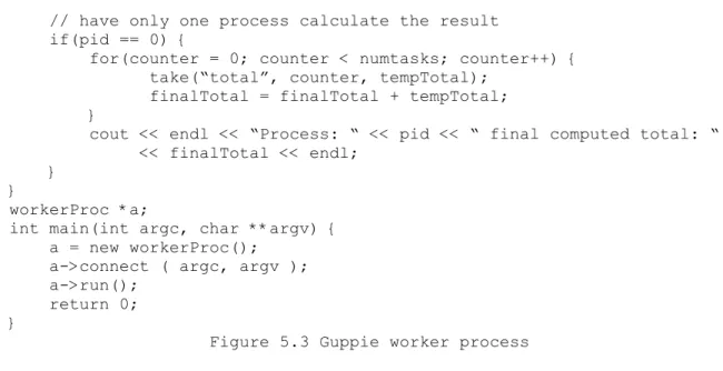
void workerProc::run() {
int size = 10000, numtasks = 4, total = 0, finalTotal = 0; int pid, counter, tempTotal, myArray[size];
take(“task”, 0, pid); // initialize array
for(counter = 0; counter < size; counter++) myArray[counter] = counter;
// have every process calculate their share for(counter = (size/numtasks)*pid;
counter < ((size/numtasks)*pid + (size/numtasks)); counter++) total = total + myArray[counter];
// have every process store its total in the tuple space cout << endl << “Process: “ << pid << “ individual total: “ << total << endl;
set(“total”, pid, total);
// have only one process calculate the result if(pid == 0) {
for(counter = 0; counter < numtasks; counter++) { take(“total”, counter, tempTotal);
finalTotal = finalTotal + tempTotal; }
cout << endl << “Process: “ << pid << “ final computed total: “ << finalTotal << endl;
} }
workerProc *a;
int main(int argc, char **argv) { a = new workerProc();
a->connect ( argc, argv ); a->run();
return 0; }
Figure 5.3 Guppie worker process
The above code creates a class called “workerProc” and allows this class to have
access to all of the main worker functions. The class “workerProc” has one class function, “run”, which is where the user writes the parallel application. In the main function, the class is created, and the “connect” function is called. The “connect”
function is a part of the main worker file, worker.cpp, and is responsible for connecting the worker process with the master process so that communication between this process and the master is possible. After the connection has been established, the “run” function is called, which is where the actual parallel application code is written.
This parallel application solves the exact same problem as seen in the OpenMP and MPI examples. The master process creates four worker processes, and each worker process executes the code within the “run” function. Each worker process initializes its own copy of the array, “myArray”. For demonstration purposes, the array has been
initialized to contain all 10000 elements, even though each process is only working with 2500 elements. The array was initialized in this format for demonstration purposes, to
stay consistent with the OpenMP and MPI code, and to better show afterwards how each process only works with a segment of the array for the parallel computation of the problem.
Once each process initializes the array, it performs its segment of code based on the process id. Because four worker processes are used in this application, the first worker process computes through locations 0 to 2499 of the array, the second worker process computes through locations 2500 to 4999 of the array, the third worker process computes through locations 5000 to 7499 of the array, and the fourth worker process computes through locations 7500 to 9999 of the array. Once each process has calculated its total, the total is stored in the tuple space using Guppie’s set(t) operation. The
following tuples are stored in the tuple space using Guppie’s set(t) function:
Worker process 0: set(“total”, pid, total), where pid = 0, total = 3123750 Worker process 1: set(“total”, pid, total), where pid = 1, total = 9373750 Worker process 2: set(“total”, pid, total), where pid = 2, total = 15623750 Worker process 3: set(“total”, pid, total), where pid = 3, total = 21873750 The programmer could choose to use the add function rather than the set function. The add function is intended to store multiple tuples in the tuple space in a queuing format, which should be based on having the same name and id parameters and a different value parameter. The following tuples could be stored in the tuple space using the add(t) function rather than the set(t) function:
Worker process 0: add(“total”, 0, total), where total = 3123750 Worker process 1: add(“total”, 0, total), where total = 9373750 Worker process 2: add(“total”, 0, total), where total = 15623750
Worker process 3: add(“total”, 0, total), where total = 21873750
After each process sets a tuple containing the finished total into the tuple space, it is necessary for one worker process to collect the tuples and calculate the overall total of the four values stored in the tuple space. This is performed in a similar manner to MPI. All that is needed is an if statement to be true for only one process. That process, process 0 in this case, retrieves the tuples from the tuple space and calculates the overall total. This is performed by using Guppie’s get(s) or take(s) function. For this application, there
is no reason to leave the tuples in the tuple space, so take(s) is a logical choice. Worker process 0 calls the take function four times because there are four worker processes that each stored an individual tuple in the tuple space. The following for loop is constructed to call the necessary take(s) functions:
for(counter = 0; counter < numtasks; counter++) { take("total", counter, tempTotal);
finalTotal = finalTotal + tempTotal; }
Each call to take fetches a tuple matching “total” and counter and stores a value into
tempTotal. After each take function executes, tempTotal is added to finalTotal. Process 0 withdraws the tuples and their values in the following order:
take(“total”, counter, tempTotal), where counter = 0, tempTotal contains 3123750 after the take operation
take(“total”, counter, tempTotal), where counter = 1, tempTotal contains 9373750 after the take operation
take(“total”, counter, tempTotal), where counter = 2, tempTotal contains 15623750 after the take operation
take(“total”, counter, tempTotal), where counter = 3, tempTotal contains 21873750 after the take operation
After all four take functions are performed and the final total has been calculated, the variable “finalTotal” contains the value 49995000.
Guppie’s four main operations, set, add, get, and take are similar to MPI’s
functions in that they can be used for communication. However, the Guppie functions are much easier to use. The programmer does not have to specify explicitly the variable’s type, how many bytes need to be used, what process is to receive the data, what process is to send the data, a tag to keep messages from being sent and received by processes not intending on sending or receiving the data, a communicator, or a variable to maintain the message’s status. The master, worker, and buffer classes handle all of those steps for the
programmer.
Guppie makes it easy to implement an application that uses the “bag of tasks” programming paradigm. The bag of tasks paradigm is a parallel computing method in which tasks are placed in a bag shared by worker processes. In Guppie, the tuple represents the bag, and the tuples represent the tasks. Each worker process repeatedly takes a task tuple from the tuple space, executes it, and possibly generates new task tuples to be placed into the tuple space to be retrieved by other worker processes. Matrix
multiplication is an example using the bag of tasks paradigm. For example, suppose three matrices of equal size are to be multiplied. Matrix X is multiplied by matrix Y, and matrix Z is multiplied by the result of X * Y. In order to compute the result for row R and column C, a worker process only needs to know the R row values from the first matrix and the C column values from the second matrix. In Guppie, once a value has been calculated, that value can be stored in the tuple space with a logical name and id. For example, the calculated value for the first row of X times the first row of Y could be