Assessing the Number of Components in Mixture Models: a Review.

F E P W O R K I N G P A P E R S

F E P W O R K I N G P A P E R S

Assessing the Number of

Assessing the Number of

Components in Mixture Models

Components in Mixture Models

: a

: a

Review

Review

Ana Oliveira-Brochado

and

Francisco Vitorino Martins

Research – Work in Progress – n. 194, November 2005

A

SSESSING THE

N

UMBER OF

C

OMPONENTS IN

M

IXTURE

M

ODELS

:

A

R

EVIEW

.

Ana Oliveira-Brochado Francisco Vitorino Martins

([email protected]) ([email protected]) Faculdade de Economia, Universidade do Porto

Rua Dr. Roberto Frias, 4200-464 Porto, Portugal.

ABSTRACT

Despite the widespread application of finite mixture models, the decision of how many classes are required to adequately represent the data is, according to many authors, an important, but unsolved issue. This work aims to review, describe and organize the available approaches designed to help the selection of the adequate number of mixture components (including Monte Carlo test procedures, information criteria and classification-based criteria); we also provide some published simulation results about their relative performance, with the purpose of identifying the scenarios where each criterion is more effective (adequate).

Key words: Finite mixture; number of mixture components; information criteria;

simulation studies.

1 Introduction

Models for mixtures of distributions, first discussed by Newcomb (1886) and Pearson (1894), are currently a very popular statistical-model base to clustering. They have been of considerable interest in recent years, leading to a vast number of both methodological developments and applications in such different scientific areas as marketing, economics, agriculture, biology, genetics, medicine or astronomy. However, despite the widespread use of finite mixture models, the decision of how many clusters are required to adequately represent the data is, according to many authors, (as Bozdogan, 1992; Bozdogan, 1994; Dillon and Kumar, 1994; McLachlan and Basford, 1988; Wedel and DeSarbo, 1994; Wedel and Kamakura, 2000; Andrews and Currim, 2003a, 2003b) an important problem, but without a satisfactory statistical solution. In fact, with real-world data, the true number of mixture components is unknown and must be inferred from the data; unfortunately, no method has been found yet, optimal for all situations.

The purpose of this work is to review, describe and organize the available criteria designed to help the selection of the adequate number of mixture components; we also aim to discuss some published simulation results about their relative effectiveness. The plan of the study is as follows: after a brief description of the finite mixture model (point 2), we review the available approaches and criteria designed to determine the number of mixture components (point 3) and describe some published simulation designs who evaluate the performance of approximate measures; finally we provide some conclusions.

2 Mixture Model

The general model assume that the N

(

n=1,...,N

)

objects on witch a set of P

(

p=1,...,P

)

variables y_n =

( )

y_np 1, are measured arise from a population that is a mixture of a finite number (S) of mixture components, in proportions λ_s

(

s=1,...,S

)

; it is not known in advance from which class a particular observation belongs and the proportions (prior probabilities or mixture weights) satisfy the following constraints (1):

1 ₌₁

1 1 S s s λ = =

∑

, 0, λ_s ≥ s=1,...,S (1)

Given that the observation y_n belongs to class s, its conditional distribution function could be defined by (2):

(

)

n ≈ fs n s

y y θ (2)

where θ_s denotes the vector of all unknown parameters needed to characterize the specific form of the density chosen2_{; The unconditional density of observation n is}

given by (3):

(

)

(

)

1 S n s s n s s f λ f = Φ =

∑

y y θ , where Φ =

( )

λ θ, (3)

The likelihood approach has become the most frequently used method among a set of several proposed approaches (Dillon e Kumar 1994; McLachlan and Peel, 2000) to estimate the vectorΦ =

( )

λ θ, . The likelihood for Φ can be formulated as (4):

(

)

(

)

1 ; N n n L f = Φ y =

∏

y Φ (4)

An estimate of Φ can be obtained by maximizing (4) with respect to Φ, subject to the restrictions (1). After, estimates of the posterior probabilities, p_ns, that observation n (n=1,...,N) comes from class s (s=1,...,S) can be calculated, by means of Bayes’ Theorem (5).

(

)

(

)

1 s s n s ns S s s n s s f y p f y λ θ λ θ = =

∑

(5)

Despite a lot of algorithms that have been published to fit mixture models, (see McLachlan and Peel, 2000 for a review) in this work we only describe the fitting of mixture models by Maximum Likelihood (ML) estimation and via Expectation-Maximization (EM) algorithm. In fact, due to its computational simplicity, the EM algorithm, which derives its name from the two basic steps, Expectation and

2 _{Some well known distributions in the exponential family include the normal, exponential, gamma, multivariate}

Maximization, has become a very used procedure. To derive the EM algorithm for mixture data, it’s necessary to introduce unobserved data, z_ns, indicating if observation

n

(

n=1,...,N

)

belongs to cluster s

(

s=1,...,S

)

: 1z_ns = if ncomes form class s and 0

ns

z = otherwise. It is assumed that the zns is i.i.d. multinomial. Considering zns as

missing data and assuming that the observed data yn, given

(

1,...,

)

t n = zn znS

z are

conditionally independent, the log-likelihood function for the complete data (or complete log-likelihood function) can be formed by (Dempster et al., 1977):

(

)

(

)

1 1 1 1 ln ; , ln ln N S N S c ns s n s ns s n s n s L z f y z λ = = = = Φ y z =

∑∑

θ +

∑∑

(6)

This complete log-likelihood is maximized by alternating E and M-steps: in the E-step is calculated the expectation of (6) E⎡_⎣lnL_c

(

Φ; ,y z

)

⎤_⎦; in the M-step de expectation of

(

)

ln _c ; ,

E⎡_⎣ L Φ y z ⎤_⎦ is maximized with respect to λ_s, producing (7) and with respect to

s

θ , leading to independently solve each of S expressions (8):

1 ˆ ˆ λ ₌

∑

= N ns n s p N (7)

(

)

1 ln ˆ N s n s ns n s f p = ∂ ∂

∑

_θy θ (8)

Table 1 provides a description of the EM algorithm.

Table 1: Expectation-Maximization algorithm

(1) At the first step of the iteration, (h=1), initialize the procedure by fixing the number of segments S and generating a starting partition p_ns( )1 .

(2) Given ( )h ns

p , obtain estimates of λ_sby using equation (7) and of θ_susing (8). (3) Convergence test: stop if the change in the log-likelihood (4) from iteration

(

h−1

)

to iteration

( )

h is sufficient small.

(4) Increment iteration index, h← +h 1, and evaluate new estimates of the posterior

membership ( )h ns

p by (5). (5) Repeat steps 2 to 4.

As we can observe from Table 1, the specification of the number of classes is required to the algorithm initialization; usually one runs the EM algorithm to a set candidate models, defined as a function of different assumptions relatively to the number of mixture components, and then the best model is chosen according to one or more diagnosis tools. Next we review the available criteria to help the decision of how to select the number of classes to retain in a mixture model solution.

3 Approaches for assessing the number of mixture components

When applying the above models to real data, the actual number of classes,S, is unknown and must be inferred form the data; to help this decision, a great number of procedures have been proposed; in this section we provide a survey of the published criteria, organized in five groups, according to their theoretical background:

i) Hypothesis Test ii) Information Criteria iii) Classification Criteria

iv) Minimum Information Ratio and related criteria v) Other criteria

An obvious way to decide upon the number of components of a mixture model is to carry out a successive Hypothesis Tests (of the null hypothesis of S segments against the alternative hypothesis of S+1 classes), using the well-known likelihood ratio test

statistic LRTS. As regularity conditions do not hold for the mixture model, an alternative procedure is the Monte Carlo test procedure, which requires bootstrapping, in order to obtain an assessment of the p-value.

Due to the computational burden of carrying out a hypothesis test based on bootstrapping, the estimation of the order of a mixture model has been considered mainly by using a penalized form of the log-likelihood function; as the likelihood increases with the addition of a component to a mixture model, some heuristics, called

Information Criteria, attempt to balance the increase in fit obtained against the larger number of parameters estimated for models with more clusters.

Although Information Criteria account for over-parametrization as large numbers of clusters are derived, it is also important to ensure that the segments are sufficiently

separated for the selected solution. To access the ability of a mixture model to provide well-separated clusters, an entropy statistic can be used to evaluate the degree of separation in the estimated posterior probabilities. These approach yields the

Classification Criteria.

The Minimum Information Ratio (MIR) criteria include functional validities specific

to the context of mixture analysis but aren’t also penalized log-likelihood methods. They are inspired on the properties of the information ratio matrix (thus the designation MIR, Minimum Information Ratio). When the EM algorithm is used to obtain parameters estimates, these criteria can be calculated as a function of the convergence rate of the EM algorithm. These criteria are isolated in a specific group due to this computation property.

The group Other Criteria includes approaches not classified in the previous classes, comprising approaches such as graphical diagnosis tools or cross-validation.

3.1 Hypothesis test: Bootstrapping the LRTS

A starting way to approach the problem of testing for the adequate number of mixture components is to carry out a hypothesis test, using the likelihood ratio test statistic (LRTS). Consider the null hypothesis H₀ of s₀ classes against the alternative hypothesis H₁ of s₁ segments: 0 0 1 1 1 0 1 0 : : , s 1 H S s H S s s s s = = > = + (9)

Under appropriate regularity conditions, the likelihood ratio test statistic, LRTS, (10) provides the necessary information to choose between these two models.

( )

( )

0

{

( )

1

( )

0

}

1

ˆ

ˆ ˆ

2log 2log 2 log log

ˆ S s s S L L L L λ ⎡⎢ ⎤⎥ − = − = − ⎢ ⎥ ⎣ ⎦ θ θ θ θ (10)

It is common to conduct successive tests and keep adding one component until the increase in the log likelihood starts to fall away as S exceeds some threshold.

Unfortunately, with mixture models, the standard LRTS does not apply, because regularity conditions do not hold3 _{for (10) to have its usual asymptotic null distribution}

of chi-squared with degrees of freedom equal the difference between the number of parameters under the null and alternative hypothesis (Aitkin and Rubin, 1985, Ghosh and Sen, 1985, Li and Sedransk, 1988, Titterington, 1990, Böhning et al,. 1994). A lot of both theoretical conjectures and simulation results have been published about the null distribution of the LRTS (see Wedel and Kamakura, 2000 or McLachlan and Peel, 2000, for a survey of these studies). According to Bozdogan (1994: 80) “To insist to use the LR test in determining the number of component clusters is fruitless, and moreover, it seems to be wrong, since the null hypothesis tested corresponds to the boundary rather than interior of the parameter space”. An alternative methodology for selecting the number of components is the Monte Carlo test procedure (Hope, 1968), applied to mixture problems by Aiktin et al. (1981), McLachlan (1987) and De Soete and DeSarbo (1991). In this procedure, the likelihood ratio statistic from the real data is compared with the values that it assume in a set of bootstrapped samples, generated under the null hypothesis. Discussions about the p-value required for this test are discussed in Hoaglin (1985), Smyth (2000), Efron and Tibshirani (1993) and McLachlan and Peel (2000). The main limitation of bootstrapping of the LRTS procedure relates to its computational demand (McLachlan e Basford, 1988; Wedel e DeSarbo, 1994; Wedel e Kamakura, 2000), leading to another class of criteria to investigate the number of mixture components, called information criteria in model selection.

3.2 Information Criteria

The likelihood, interpreted as a measure of the quality of the adjustment, could not be used as a criterion to select the number of components in a mixture model due to its tendency to systematic select more complex solutions, with a higher number of parameters (classes). The so called Information Criteria impose a penalty on the likelihood that is related to the number of parameters estimated, thus assuming the general form (11): ( ) ( ) IC_s = −2lnL+dk_s (11) 3 0

where k_{( )s} is the number of parameters associated to a solution with S clusters and d is some constant or the “marginal cost” per parameters (Bozdogan, 1987). Information Criteria is a general family, including criteria that are estimates of (relative) Kullback-Leibler distance, approaches that have been derived within a Bayesian framework for model selection and “consistent criteria”.

3.2.1 KULLBACK-LEIBLER DISTANCE ESTIMATORS

According to Bozdogan (1987: 346) “Akaike, in a very important sequence of papers Akaike (1973, 1974, 1977) was perhaps one of the first who laid the foundation of the modern field of statistical data modelling, statistical model identification and validation”. The imaginative work of Akaike lies in the relation found between the relative expected Kullback-Leibler distance (Kullback and Leibler, 1951), considered by the author as a fundamental basis for model selection, and its proposed estimator, the maximized log-likelihood. This relation leads to a general methodology to selecte a parsimonious model. The Kullback-Leibler quantity, I, or, equivalently, the generalized entropy of Boltzman, B, measure de distance between one model and its true distribution. Of course, good inference procedures will make this distance as small as possible.

AIC

Akaike´s Information Criterion, AIC (Akaike, 1973, 1974, 1977, 1984) is an estimator of minus twice the negentropy or twice the Kullback-Leibler distance. From Akaike (1973) and Bozdogan (1987, 1994) we can recall that, for a large sample size, a measure of the average estimation error is given by the expectation of the Kullback-Leibler Information (between one model, characterized by the parameters θˆ_k and the true model, denoted by _θ*_):

(

ˆ

)

(

ˆ

)

2NE I⎡⎣ θ θ*, k ⎦⎤= −2NE B⎡⎣ θ θ*, k ⎤⎦≅ +δ k (12) where * ˆ 2 k F N

δ = θ −θ represents an unknown bias term, where the square norm is taken with respect to the Fisher Information matrix and k, the number of free parameters in the estimated model.

Akaike (1973, 1974) estimates δ based on the Wald results for the distribution of the LRTS.

Based on the alternative hypothesis that * ˆ

K

=

θ θ , Wald (1943) concludes that (13) is asymptotically distributed has a noncentral _χ2 _{random variable, with} *

v = −K k degress of freedom and the noncentrality parameter δ (14).

( )

( )

{

ˆ ˆ

}

2logλ 2 lnL _K lnL _k − = θ − θ (13)

( )

2 * 2logλ χ δ_v − ≈ (14) As is well known,

[

]

2

( )

2logλ E 2logλ E⎡χ δv ⎤= + δ v − ≅ − _{= ⎣ ⎦} (15)

Solving (15) in relation to δ and substituting the result in (12) we obtain:

(

ˆ

)

2NE I⎡_⎣ θ θ*, _k ⎤ ≅ −_⎦ 2lnλ− +v k (16)

Ignoring the constant terms in (12) AIC is defined by:

AIC= −2logL+2k (17)

AIC3

Bozdgoan (1994) propose a modified version of AIC, designed to handle with mixture data. Relatively to AIC derivation, a new assumption for the distribution of the LRTS is assumed, based on Wolfe’s work (Wolfe, 1970, 1971).

2

( )

*

2 logC λ χ δv

− ≈ (18)

where the degrees of freedom are * ₂

(

)

v = K−k , δ is the noncentrality parameter, and C a correction factor. The new criteria, labelled as Modified AIC (Bozdogan, 1994), is also known as AIC (19). ₃

3

AIC = −2lnL+3k (19)

AIC4

Bozdogan (1994) obtain another information criteria, using the asymptotic relationship between noncentral chi-square distributions given by Kendall and Stuart (1979), namely

*

2 _ρ 2

k v

χ ≈ χ (20)

where ρ is a multiplicative constant (21) * * 2 v v δ ρ δ + = + (21)

As the noncentrality parameter or the bias gets larger between the models, ρ→2 in the limit in (21), and we obtain:

( )

* 2 ₂ 2 k v χ δ ≈ χ (22) and

( )

2 2 2 2 _k 2 _k 2 _s E_⎣⎡ χ _⎦⎤= E_{⎣ ⎦}⎡ ⎤χ = k=Var χ (23) So we can write,

(

* ˆ

)

2nE I⎡⎣ θ θ; s ⎤ ≅ +⎦ δ 2k (24)

We can further obtain 4

AIC = −2logL+4k (25)

AICc – A Small sample AIC

Sugiura (1978) and Hurvich and Tsai (1989, 1995) conclude that AIC may perform poorly, conducting to overfitting, if there are too many parameters in relation to the sample size. According to (Hurvich e Tsai 1989: 298), “As k, de dimension of the candidate model, increases in comparison to N, the sample size, AIC becomes strongly negatively estimate of the K-L information. This bias can lead to overfitting”. They derived a small-sample bias adjustment, which led to a criterion calledAIC_c (26).

AIC 2log 2 1 ⎛ ⎞ = − + _{⎜ ⎟} − − ⎝ ⎠ c N L k N k (26)

Note that the penalty term in AIC is multiplied by the correction factorN

(

N− −k 1

)

;

AICc can be rewritten as:

(

)

2 1 AIC 2log 2 1 + = − + + − − c k k L k N k (27) or, equivalently,

(

)

2 1 AIC AIC 1 + = + − − c k k N k (28)

Generaly, AICc is recommended when the ration N K is less than 40 (Burnham e Anderson, 2002).

QAIC and QAICc – Modification of AIC for overdispersed count data

The modification of AIC criterion for overdispersed count data is known as QAIC

Quasi-likelihood Akaike Information Criterion (Lebreton et al., 1992):

ˆ

QAIC= −2logL c+2k (29)

where c is a single inflation factor, that can be estimated from the goodness-of-fit chi-square statistic of the model with the higher number of supposed components and its degrees of freedom, df :

df

cˆ=χ2 (30)

We might expect values of c between 1 and 4; larger values of c reveal an inadequate model structure. For small samples, N k<40, the authors propose to adjust the QAIC

criterion by same correction proposed to derive AIC_c.

(

)

2 1 ˆ QAIC 2log 2 1 + = − + + − − c k k L c k n k (31)

Note that when c=1, QAIC is equivalent to AIC (Akaike, 1973) and QAICc reduces do

AICc.

TIC

Takeuchi (1976) proposed, three years after the pioneering work of Akaike (1973), a knew information criterion, named by TIC, Takeuchi’s Information Criterion; despite

being little-known and rarely applied (note that the original paper is in Japanese), it possess an interesting application context: it was thought to be useful in cases where the candidate models were not particularly close approximations of the true model. According to Burnham and Anderson (2002: 65), “One might consider always using TIC and worry less about the adequacy of the models in the set of candidates”. TIC, which has a more general bias-adjustment term, is defined by (32):

_{= −2ln 2 ⎡} −1_⎤

+ ⋅ ⎣ ⎦

Matrices I e F represent the first and second mixed partial derivatives of the log-likelihood function and trdenotes the matrix trace function.

EIC Efron (bootstrapped Information Criterion)

Ishiguro et al. (1997) developed a new extension of AIC, called EIC Efron (bootstrapped) Information Criteria. The bias term is estimated using Efron’s (1979) bootstrap. The number of mixture components is chosen on the basis of (33).

( )

ˆ

EIC= −2logL+2b E_N (33)

Where the (nonparametric) bootstrap bias b E

( )

ˆn is approximated by Monte Carlo

methods on the basis of B bootstrap samples.

( )

(

* *

)

(

*

)

1 1 1 _ˆ 1 _ˆ ˆ N _{log ;} N _{log ;} n n n n n b E E f Y f Y N = θ N = θ ⎧ ⎫ = _⎨ − _⎬ ⎩

∑

∑

⎭ (34)

where _θˆ* _{denotes the MLE obtained from the bootstrap sample.} . . . * * 1 ,..., ˆ i i d N N Y Y ≈ E (35)

It’s possible to approximate this bootstrap bias on the basis of B independent bootstrap samples

(

)

. . . * * 1 ,..., ˆ 1,..., i i d b Nb ≈ EN b= B Y Y . (36) Consider ˆ* b

θ as the MLE formed from the bth bootstrap sample

(

b=1,...,B

)

. This gives:

( )

(

* *

)

(

*

)

1 1 1 1 1 _ˆ 1 _ˆ ˆ B N _{log ;} N _{log ;} N nb b n b b n n b E f y f y B = N = θ N = θ ⎧ ⎫ ≈ _⎨ − _⎬ ⎩ ⎭

∑ ∑

∑

(37) .

3.2.2 BAYESIAN-BASED INFORMATION CRITERIA

We now consider some criteria that have been derived within a Bayesian framework for model selection. In a Bayesian framework, the model with the highest posterior probability is chosen among S competing models. According to Bayes’s theorem, the posterior probability of Model Ms (s=1,...,S) given the data y is (38):

(

)

(

)

( )

(

)

( )

1 s s s S s s s p M p M p M p M p M = =

∑

y y y , 1,...,s= S (38)

where p

(

y M_s

)

is the integrated likelihood of the model M_s and P M

( )

_s is its prior probability. When models are equally probable a priori, the model with the highest posterior probability corresponds to the model with the highest integrated likelihood (39).

(

s

)

( ) ( )

p y M =

∫

L Φ p Φ Φd (39)

Where p

( )

Φ is a non informative prior distribution on Φ for the model M_s.

BIC

The main Bayesian-based information criteria, proposed by Schwarz (1978) use an approximation of the integrated likelihood, yielding the Schwartz Criteria:

(

)

ln ln ln 2 ≈ − s k p y M L N (40)

Kass e Raftery (1995) note that minus twice the Schwartz Criteria is often named by the Bayesian Information Criteria (BIC) as in (41).

2 ln ln

BIC= − L+k N (41)

Curiously, BIC (41) was also derived in the context of coding theory by Rissanen (1986, 1987, 1989), and known by MDL, Minimum Decription Lenght.

AWE

Banfield and Raftery (1993) derived another criterion in the context of Bayesian theory, the AWE Approximate Weight of Evidence. Contrasting with BIC, that is a general tool for model selection, AWE (42) was developed specifically as a tool to select the optimal number of components in a mixture of normal distributions and uses the Complete Likelihood Function (6) 3 2ln ln 2 C AWE= − L +K⎛_⎜ + N⎞_⎟ ⎝ ⎠ (42)

When mixture components are well separated it can be expected an analogous behaviour for BIC and AWE (Celeux and Soromenho, 1996).

Other Bayesian criteria

Other approximations have been proposed to approximate the integrated likelihood, namely the Laplace-Metropolis Criterion, Laplace empirical criterion and the Laplace Method of Approximation (Bass and Raftery, 1995; McLachlan and Peel, 2000).

3.2.3 CONSISTENT CRITERIA

CAIC and CAICF

Bozdogan (1992) provides two analytic extensions of AIC, without violating Akaike´s principle of minimizing the Kulback-Leibler information quantity. The new selection criteria, called Consistent AIC – CAIC, and Consistent AIC with Fisher Information - CAIF, make AIC asymptotically consistent and penalize overparametrization more stringently.

To make AIC consistent, Bozdogan (1992) defines *

v as an increasing function of the sample size. Considering *

(

)

_ln

v = K−k N, instead of v*=

(

K−k

)

used to derivate AIC, we obtain:

(

)

CAIC= −2logL+k⎡_⎣ logN +1⎤_⎦ (43)

The criterion CAICF incorporates the Fisher Information matrix within the penalty component.

(

)

CAICF -2 logL log 2 log AIC log log

k N k N ⎡ ⎤ = + _⎣ + _⎦+ = + + F F (44) HQ

Hannan and Quinn (1979) provided a consistent model selection criterion, where the penalty term increases with the sample size(45):

(

)

HQ= −2lnL ck+ ln lnN (45)

where c is a constant greater or equal to 2. This criterion, despite being often cited, has little use in practice; Oliver et al. (1999) rewrite HQ for the context of mixture models and include it in their experiment.

ICOMP

Bozdogan (1988, 1990, 1993, 1994) developed the complexity criterion, ICOMP, for model selection. Analytic formulation of ICOMP, despite taking the “spirit of AIC” (Bozdogan, 1994), is based on the generalization and use of an entropic covariance complexity index of van Emden (1971).

(

)

( )

1 1

ICOMP Overall Model 2log ln ln

− − ⎡ ⎤ ⎢ ⎥ = − + − ⎢ ⎥ ⎣ ⎦ tr L k k F F (46)

So, in the context of mixture models, the derivation of ICOMP (46) requires the knowledge of the inverse-Fisher information matrix (IFIM) of the model and its sample estimate. According to Windham and Cutler (1994), the Fisher Information matrix could be estimated using (47) or (48).

(

)

2 ˆ 2 1 log 1 ˆ N n n L N ₌ = ⎛_∂ ⎞ = − ⎜_⎜ ⎟_⎟ ∂ ⎝ ⎠

∑

θ θ y θ F θ (47)

(

)

(

)

ˆ ˆ 1 log log 1 ˆ N n n t n L L N ₌ = = ⎛∂ ∂ ⎞ = − ⎜_⎜ ⎟_⎟ ∂ ∂ ⎝ ⎠

∑

θ θ θ θ y θ y θ F θ θ (48)

Given the difficulties of estimating _F−1 _{for a mixture model, Bozdogan (1993, 1994)} propose some approximation to the case of Gaussian mixtures, using the expected information matrix to a classified sample.

ICOMP tends to penalize models that produce high variances in the parameter estimates (through the second term in (46)) and models with more parameters (the Hessian becomes near-singular due to increasing number of parameters and the value of the third term increases).

3.3 Classification-based information criteria

The classification criteria considered in this session measure the ability of a mixture model to provide well-separated clusters. Some measures are derived in the context of mixture models and others are “imported” from the fuzzy literature (Bezdek et al.,

1997). These criteria are named, respectively as probabilistic indices and fuzzy indices4_.

3.3.1 PROBABILISTIC INDICES

LP and E

Biernacki (1997) propose the use of the criterion LP (49), the logarithm of the probability of the partition z when all the posterior probabilities p_ns are known, and the Entropy Criterion, E (50), to compare solutions with different number of clusters in mixture models. 1 1 LP log = = = −

∑∑

S N _{ns ns} s n z p (49) 1 1 E ln = = = −

∑∑

N S ns ns n s p p (50)

Note that z_ns =1 if arg max _nt

t p =s and 0, otherwise. If the mixture components are well

separated, the fuzzy classification matrix P=

[ ]

p_ns tends to define a partition and both (49) and (50) assume small values (≈0);

CLC

Biernacki and Govaert (1997), proposed the classification likelihood criterion, CLC (51) to choose the number of classes in a mixture of normal distributions, based on the relation (52).

(

)

1 1 log S N ns s s n s s n CLC z λ f y = = ⎡ ⎤ =

∑∑

_⎣ θ _⎦ (51) CLC log= L−LP (52)

where LP is defined by (49).So, the classification likelihood (or the complete log-likelihood) is the standard likelihood penalized by a term which measures the quality of the partition, thus making a compromise between the fit of the data and the ability of the

4 _{The quantities}

ns

p are interpreted as partial memberships in the context of fuzzy clustering and as probabilities of membership in the context of mixture models.

mixture model to provide a classification (Biernacki, 1997; Biernacki and Govaert, 1997).

CL

Biernacki (1997) and Biermacki and Govaert (1997) propose the following criteria to select the number of mixture components, named by classification log-likelihood, CL (53):

(

)

1 1 CL log λ = = ⎡ ⎤ =

∑∑

S N _{ns ⎣ s n s ⎦} s n p f y θ (53)

The defined criteria can be calculated on the base of the relation defined by Hathaway (1986), who provides a decomposition of the log-likelihood function into two terms (54)

lnLS =CL E+ (54)

where E , defined by (50), measures the overlap of the mixture components and is related to the fuzzy classification matrix; relation (54) reveals that the classification log-likelihood also can be interpreted as a compromise between the fit of the data to the mixture model (first term) and the ability of the mixture model to provide well-separated clusters (second term).

NEC

The quantity (50) is also the basis for the Normalizez Entropy Criterion NEC, provided by Celeux and Soromenho (1996); from the Hathaway’s relation (54), we can write:

( ) ( ) ( ) ( ) ( ) ( ) ( ) 1 1 1 1 , 1 ln ln ln ln − = + > − − s s s s CL CL E s L L L L (55)

where lnL_{( )1} denotes the maximized log-likelihood for a single distribution.

So, the normalized entropy criterion to be normalized to assess the number of mixture components is defined as (56): ( ) ( ) ( ) ( )1 ln ln = − S S S E NEC L L (56)

However, as NEC is not valid to decide between one and more than one clusters, Biernacki (1999) presents an extension of this criterion to deal with this situation.

ICL-BIC

Biernacki et al. (2000) note that the integrated likelihood does not account the ability of the mixture model to provide evidence for a clustering structure in the data and suggest the alternative use of the Integrated Completed likelihood(57):

(

, _s

)

_c

( ) ( )

p y z M =

∫

L Φ p Φ Φd (57)

To approximate (57) Biernacki et al. (2000) propose the use of a BIC-like approximation.

(

)

( )

ln , ln ln 2 s c k p y z M ≈ L Φ − N (58) Substituting (52) in (58), we obtain:

( )

ln ln 2 k ICL≈ L Φ −LP− N (59)

The criteria ICL−BIC is thus defined by:

2ln 2 ln

ICL−BIC= − L+ LP+k N (60)

EP

Ramaswamy et al. (1993) propose another entropy-based measure to assess the degree of fuzziness in the fuzzy partition matrix, based on the posterior probabilities.

1 1 ln 1 ln = = − = −

∑∑

N S ns ns n s s p p E N S (61) s

E is bounded between 0 (meaning that all the posterior probabilities are equal to each object) and 1 (corresponding to minimum entropy). As EM_s is a nonlinear measure, Jedidi et al. (1996) argument that values for the indicator between 0,5 and 0,6 can reveal a enough separation.

3.3.2 FUZZY INDICES

PC and PE

Bezdek (1981) developed the criteria ‘Partition Coeficient’ - PC and ´Partition Entropy’ – PE, to select the optimal number of clusters when the fuzzy k-means algorithm (Bezdek, 1974, Dunn 1974) is used; recently, Windham e Cutler (1992) proposed the

use of the PC to select the number of components in mixture models and Bezdek et al. (1997) motivated the use of both indicators. The PC criteria is defined as (62):

2 1 1 PC₌

∑∑

= = N S ns n s p N (62)

This indicator assumes values in the domain1S ≤PC 1≤ , where the lower bound and

upper bound are associated, respectively, to a completely fuzzy solution and a nonoverlapping solution; this criterion presents the limitation of not allowing the test of

1

S= againstS>1, becausePC_(S=1) = ≥1 PC_(S>1). The Partition Entropy is defined as (63):

( )

1 1 ln PE₌

∑∑

= = N S ns ns n s p p N (63)

Being defined on the domain 0 PE ln≤ ≤ S, the PE should be minimized. 3.4 MIR criteria

The validity functionals analysed in this section are not penalized likelihood methods, and have been developed in the specific context of mixture models by Windham and Cutler (1992) and Cutler and Windham (1994).

MIR

The first measure to be analysed is the MIR, Minimum Information Ratio, introduced by Windham and Cutler (1992). MIR is defined as the smallest eigenvalue of the information ratio matrix, −1

c

F F, where F is the Fisher Information Matrix and Fc the

Fisher Information for the classified sample. According to the authors, MIR is used as a measure of the proportion of information about the parameters without knowing the subpopulation memberships and might be interpreted as the ability of the data to distinguish the component densities. When the EM algorithm is used to estimate the model parameters, MIR can be estimated by one minus the convergence rate of the EM algorithm (64); in fact, Louis (1982) and Sundberg (1976) have shown that the convergence rate of the EM algorithm is the largest eigenvalue of ₋ −1

c

I F F or,

equivalently, the smallest eigenvalues of −1

c

The convergence rate can be estimated from ratios of distances between successive iterates. 1 1 1 h h h h MIR + − − = − − θ θ θ θ (64)

Where ⋅ is a convenient norm of the Euclidean space and θh the sequence of

parameter estimates produced by the iterations of the EM algorithm.

MIR is interpreted as the ability of the data to distinguish the component densities and it take values between 0 and 1; s small MIR suggests a poor clustering and a large MIR suggests a good clustering.

Windham e Cutler (1992) propose also the procedure MIREV - Minimum Information

Ratio Estimation and Validation, as follows.

The simplicity of the estimation step makes it attractive, but summarizing the clustering quality in a single number could be dangerous. The validation step provides a measure of the reliability of the number of components selected by the estimation step.

Polymedis and Titterington (1998) proposed a modification of the MIREV Procedure; in their simulation experiment the new method outperformed the method proposed by Windham and Cutler (1992).

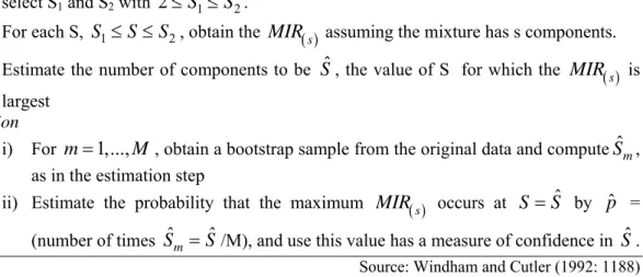
Table 2: MIREV Procedure

Estimation

i) select S1 and S2 with 2≤S1≤S2.

ii) For each S, S₁≤ ≤S S₂, obtain the MIR_{( )s} assuming the mixture has s components. iii) Estimate the number of components to be Sˆ, the value of S for which the MIR_{( )s} is

largest

Validation

i) For m=1,...,M, obtain a bootstrap sample from the original data and computeSˆ_m, as in the estimation step

ii) Estimate the probability that the maximum MIR_{( )s} occurs at S=Sˆ by pˆ = (number of times Sˆ_m=Sˆ/M), and use this value has a measure of confidence in Sˆ.

ALL and AND

Two additional validity functionals could be obtained from MIR (Cutler e Windham, 1994), the adjusted log-likelihood ALL (65) and the adjusted number of components, ANC (66).

(

ln ln 1

)

s s s ALL =MIR L − L (65)

(

1

)

s s ANC = S− MIR (66)

The estimated number of components is chosen to maximize MIR, ALL and ANC. AsMIR_(S=1) = ≥1 MIR_(S>1), it can only be used to S >1.

3.5 Other criteria

EL – Elbow Likelihood

Cuttler and Windham (1992) proposed a modification of the log-likelihood, called EL – Elbow likelihood; according to EL, the estimated number of components is the smallest value of S for whichlnLs+₁−lnLs <ε, where the subscript denotes the number of

components and the value ofε is 1% the absolute value of the log-likelihood for the model with the smallest number of components.

LOGVL

Andrews and Currim (2003a,b) suggest the use of the log-likelihood value from the validation sample (LOGVL) as a criterion to select the number of classes in a mixture regression model; so, this criterion requires the split of the empirical data into two parts, an estimation sample and a validation sample. Unlike the estimation sample log-likelihood, LOGVL may decrease when the number of mixture components increase, which may suggest misspecification.

CVIC – Cross-Validation-Based Information Criterion

CVIC (Smyth 2000) suggests the use of Cross-Validation-Based Information Criterion to choose the number of mixture components. Cross validation approaches require that the empirical data is divided repeatedly (M times) into two parts: an estimation sample and a validation sample; model parameters are estimated on the estimation sample and model performance is then tested on the validation sample. The criterion proposed by Smith (2000) is defined as:

(

)

1 1 _ˆ ln ; m m M s V E m CVIC L M = =

∑

y θ (67) where ˆ m E

θ denotes the parameters estimated (for the model under S components) from the mth estimating subset, Em and lnL y

(

V_m;θˆE_m

)

is the log-likelihood evaluated on the

validation sample Vm using the parameters estimates ˆθE_m.

Different cross-validation methodologies arise, based on how the M validation and estimation samples are chosen. The so called v-fold cross validation use v disjoint validation samples, each of size N v/ ; when v=N, the approach is known as “leave-one-out” or “jacknife”; due to its time consumption, consideration might be given to

1

v> solutions, being v=10 a popular number (Smith, 2000); Another way, known as Monte Carlo Test validation, generates M independent partitions of the data, for a fixed fraction γ , into a estimation sample of size γN and a validation sample of size

(

1−γ

)

N. Smith (2000) suggests the choice γ =0,5. Smith (2000) compared CVIC (implemented via Monte Carlo methods) with BIC and the bootstrap LRTS in real data sets and concluded that these three suggest the same number of mixture components.

Gradient function

Lindsay and Roeder (1992) present two diagnostic tools, the residual function and the gradient function, useful to select the number of segments in mixture models. According to the author these two proposed functions are closely related and should be used as the first approach to mixture models validation. Due to its popularity and properties (Deb and Trivedy, 1997; Wedel and Kamakura, 2000), we limit our discussion to the gradient function.

The gradient function is defined by (68):

(

)

(

)

(

)

ˆ, 1 , * 1 ˆ, * f S d S f S S ⎡ ₌ ⎤ ⎢ ⎥ =_⎢ − _⎥ = ⎢ ⎥ ⎣ ⎦ yθ y yθ (68)

Following Lindsay and Roeder (1992), the graph of (68) could be used as a diagnostic test for the presence of the mixture: the convexity of the graph is interpreted as evidence in favour of a mixture. However, as such convexity could be observed for more than one value of S, the analysis of other information criteria is also required.

An additional diagnosis(69) suggested by Linday and Roeder (1992) is a weighted sum of equation (68).

( )

(

) ( )

1 1 * , * = = =

∑∑

N S n s D S d y S f y (69)

Where f

( )

y is the sample frequency of y. Deb and Trivedi (1997) applied (68) and (69) in the context of mixture regression models.

4 Empirical comparisons of performance

Despite the large number of heuristics available to help the selection of the optimal number of mixture model components, few studies have been conducted in order to evaluate their relative effectiveness.

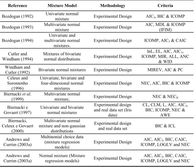
In fact, the majority of results appear in papers where a new criterion is proposed and an experimental design is conducted in order to compare its performance with a limited number of well-known criteria; these studies do not intent to provide general results, but also illustrate the effectiveness of the new developed criteria (Bozdogan, 1987, 1992, 1994; Windham and Cutler, 1992; Celeux e Soromenho, 1996; Biernacki et al, 1999; Smith, 2000); only few contributions defined as main objective to compare criteria designed for mixture model selection (Bozdogan, 1992, 1994, Cutler and Windham, 1994, Biernacki, 1997, Hawpkins, 2001, Andrews and Currim, 2003a,b). Additionally, in general these studies consider a limited number of data characteristics (mostly multivariate normal data with no predictors) and manipulated factors (number of components, separation degree) in the experimental design. Exceptions are the full factorial designs developed by Andrews and Currim (2003a,b) in the context of mixture models and the work of Cutler and Windham (1994). Finally, available studies yield different conclusions about the overall performance of the compared criteria. Table 3 provides a summary of some studies where the performance of criteria is evaluated and compared.

Table 3: Empirical comparisons of performance

Reference Mixture Model Methodology Criteria

Bozdogan (1992) Univariate normal _mixture Experimental Design AIC3, BIC & ICOMP

Bozdogan (1993) Multivariate normal _mixture Experimental Design AIC, MDL & ICOMP _(IFIM) Bozdogan (1994) multivariate normal Univariate and

mixtures. Experimental Design ICOMP, AIC3 & CAIC Cutler and

Windham (1994) Mixtures of bivariate normal distributions Experimental Design

lnL, EL, AIC, AIC3,

ICOMP, MIR, ALL, ANC & WID

Windham and

Cutler (1992) Bivariate normal mixtures Experimental Design MIREV, AIC & PC Celeux and

Soromenho (1996)

Univariate, bivariate and four-dimesional normal

mixtures Experimental Design NEC, AIC, BIC & ICOMP Biernacki et al.

(1999) Multivariate normal mixture, Experimental Design NEC & NECII

Biernacki e Govaert (1997)

Univariate and bivariate normal mixtures

Experimental design and real data set (Iris

data)

CL, CLM, L, AIC, AIC3,

BIC, ICOMP, NEC & AWE Biernacki,

Celeux e Govaert (2000)

Multivariate normal mixture and non-gaussian

distributions

Experimental design

and real data set BIC & ICL Andrews and

Currim (2003a)

Multinonial choice data (mixture regression

models) Experimental Design

AIC, AIC3, BIC, CAIC,

ICOMP, LOGLV and NEC Andrews and

Currim (2003a)

Normal mixture (Mixture

regression models) Experimental Design

AIC, AIC3, BIC, CAIC,

ICOMP, LOGLV and NEC

5 Conclusion

This work reveals the existence of a large number of available criteria designed to help the selection of the adequate number of clusters to retain in mixture models; some of these approaches possess a powerful theoretical justification, while others are based in more empirical arguments. The literature was organized in five groups, namely: hypothesis test in the context of mixture models; information criteria, including those criteria that penalize the over-parametrization, (including KL estimators, bayesian criteria and consistent criteria); classification-based criteria, include both criteria developed in the context of mixture analysis and criteria imported from the fuzzy classification literature that look for well-separated clusters); MIR and related criteria that are calculated using the convergence rate o the EM algorithm and other criteria.

Review of published simulation studies about the effectiveness of the available criteria shows that few comprehensive studies have been conducted. In general studies tend to be narrow in scope, and aim to exemplify the effectiveness of new proposed measures rather than compare the effectiveness of available measures. Also, as the majority of these studies have appeared mostly in the statistics literature, we don’t know if the experimental designs include all relevant manipulated factors for specific areas of application. Finally, as results of available studies aren’t completely consistent, it may be that no criterion is best for all types of mixtures in all contexts.

References

Aitkin, M., Anderson, D. and Hinde, J. (1981). “Statistical Modelling of Data on Teaching Styles (with discussion)”. Journal of the Royal Statistical Society B, 144: 419-461.

Aitkin, Murray and Runin, Donald (1985). “Estimation and Hypothesis Testing in Finite Mixture Models.” Journal of the Royal Statistical Society B, 47 (1): 67-75. Akaike, H. (1974). “A New Look at the Statistical Model Identification.” IEEE

Transactions on Automatic Control, AC-19 (6): 716-723.

Akaike, H. (1973). “Information Theory as an Extension of the Maximum Likelihood Principle”. In Second International Symposium on Information Theory, B.N. Petrov and F. Csaki, Akademiai Kiado, (Eds.) Budapest, pp. 267-281.

Akaike, H. (1977). “On Entropy Maximization Principle”. In Proceedings of the Symposium on Applications of Statistics, P. R. Krishnaiah (Eds.), Amsterdam: North-Holland, pp. 27-47.

Akaike, H. (1984). “A New Look at the Statistical Model Identification”. IEEE Trans. Automatic Control, 19: 716-723.

Andrews, R. L. and Currim, I. S. (2003a). “A Comparison of Segment Retention Criteria for Finite Mixture Logit Models.” Journal of Marketing Research, XL: 235-243.

Andrews, R. L., and Currim, L. S. (2003b). “Recovering and Profiling the True Segmentation Structure in Markets: an Empirical Investigation.” International Journal of Research in Marketing, 20: 177-192

Banfield, J. D. and Raftery, A. E. (1993). “Model- Based Gaussian and Non-Gaussian Clustering”. Biometrics, 49 (3): 803-821.

Bezdek, J. C. (1974). “Numerical Taxonomy with Fuzzy Sets”. Journal of Mathematical Biology, 1: 57-71.

Bezdek, J. C. (1981). Pattern Recognition with Fuzzy Objective Function Algorithms. Plenum Press.

Bezdek, J. C., Li, W. Q., Attikiouzel, Y. and Windham, M. (1997). “A Geometric Approach to Cluster Validity for Normal Mixtures”. Soft Computing, 1: 166-179.

C. Biernacki (1997). Choix de modèles en classification. Ph.D. Thesis, Université de Technologie de Compiègne. [http://www-math.univ-fcomte.fr/pp_Annu/CBIERNACKI/]

Biernacki, C. and Govaert, G. (1997). “Using the Classification Likelihood to Choose the Number of Clusters”. Computing Science and Statistics, 29: 451-457. Biernacki, C., and Celeux, G. (1999). “An Improvement of the NEC Criterion for

Assessing the Number of Clusters in a Mixture Model”. Pattern Recognition Letters, 20 (3): 267-272.

Biernacki, C., Celeux, G. and Govaert, G.. (2000). “Assessing a Mixture Model for Clustering with the Integrated Completed Likelihood”. IEEE Transactions on Pattern Analysis and Machine Intelligence, 22 (7): 719-725.

Böhning, D., Dietz, E., Schaub, R., Schlattman, P. and Lindsay, B. (1994). “The Distribution of the Likelihood Ratio for Mixtures of Densities from the One-Parameter Exponential Family.” Annals of the Institute of Statistical Mathematics, 46: 373-388.

Bozdogan, H. (1987). “Model selection and Akaike´s Information Criterion (AIC): the General Theory and its Analytical Extensions”. Psychometrika, 52 (3): 345-370.

Bozdogan, H. (1988). “ICOMP: A New Model-Selection Criterion”. In Classification and Related Methods of Data Analysis, Hans H. Bock (Eds.), Amsterdam:Elsevier Science Publishers B. V. (North-Holland), pp. 599-608.

Bozdogan, H. (1990). “On the Information-Based Measure of Covariance Complexity and Its Application to the Evaluation of Multivariate Linear Models”, Communications in Statistics, Theory and Methods, A19 (1): 221-278.

Bozdogan, H. (1992). “Choosing the Number of Component Clusters in the Mixture-Model Using a New Informational Complexity Criterion of the Inverse-Fisher Information Matrix. In O. Opitz, B. LAusen and R. Klar (Eds.), Information and Classification: Concepts, Methods and Applications, New York. Springer-Verlag, pp. 44-54.

Bozdogan, H. (1993). “Choosing the Number of Component Clusters in the Mixture-Model Using a New Informational Complexity Criterion of the Inverse-Fisher Information Matrix”. In Studies in Classification, Data Analysis, and Knowledge Organization, O. Opitz, B.Lausen, and R. Klar (Eds.), Springer-Verlag, Heidelberg, pp. 40-54.

Bozdogan, H. (1994). “Mixture-Model Cluster Analysis Using Model Selection Criteria and a New Information Measure of Complexity”. In Proceedings of the Fist US/Japan Conference on the Frontiers of Statistical Modeling: An Informational Approach, H. Bozdogan (Eds.), Vol. 2, Boston, Kluwer Academic Publishers, pp. 69-113.

Burnham, K. P. e Anderson, D. R. (2002). Model Selection and Multimodel Inference. A Practical Information-Thepretic Approach. Springer.

Biernacki, C. (1997). “Choix de Modèles en Classification”. Ph.D. Thesis, Université de Technologie de Compiègne. [http://www-math.univ-fcomte.fr/pp_Annu/CBIERNACKI/]

Celeux, G. and Soromenho, G. (1996). “An Entropy Criterion for Assessing the Number of Clusters in a Mixture Model”. Journal of Classification, 13 (2): 195-212. Cutler, A. and Windham, M. P. (1994). “Information-Based Validity Functionals for

Mixture Analysis”. In Proceedings of the First US/Japan Conference on the Frontiers of Statistical Modeling: An Informational Approach, H. Bozdogan (Eds.): 149-170.

De Soete, Geert and DeSarbo, Wayne S. (1991). “A Latent Class Probit Model for Analysing Pick Any/N Data”. Journal of Classification, 8: 45-63.

Dempster, A. P., Laird, N. M. ad Rubin, Donald B. (1977). “Maximum Likelihood from Incomplete Data via the EM-Algorithm”. Journal of the Royal Statistical Society, B39: 1-38.

Deb, Partha e Trivedi, Pravin K. (1997). “Demand for Medical Care by the Elderly: A Finite Mixture Approach”. Journal of Applied Econometrics, 12: 313-336. Dillon, W. R. and Kumar, A. (1994). “Latent Structure and Other Mixture Models in

Marketing: An Integrative Survey and Overview”. In Advanced Methods in Marketing Research, Richard P. Bagozzi (Eds.), Cambridge, MA, Blackwell, pp. 295:351.

Dunn, J. C. (1974). “A Fuzzy Relative of the ISODATA Process and Its Use in Detecting Compact Well-Separated Clusters”. Journal of Cybernetics, 3: 32-57.

Efron, B. (1979). “Bootstrap Methods: Another Look at the Jackknife”. Annals of Statistics, 7: 1-26.

Efron, B. and Tibshirani, R. (1993). An Introduction to the Bootstrap. London: Chapman & Hall.

Ghosh, J. H. and Sen, P. K. (1985). “On the Asymptotic Performance of the Log Likelihood Ratio Statistic for the Mixture Models and Related Results. Proceedings of the Berkeley Conference in Honor of Jerzy Neyman and Jack Kiefer, Vol. 2, Monterey: Wadsworth: 789-806.

Hannan, E. J. and Quinn, B.G. (1979). “The Determination of the Order of an Autoregression”. Journal of the Royal Statistical Society, B41: 190-195.

Hathway, R. J. (1986). “Another Interpretation of the EM Algorithm for Mixture Distributions”. Statistics & Probability Letters, 4: 53-56.

Hawkins, D. S., Allen, D. M. and Strmberg, A. J. (2001). “Determining the number of components in mixtures of linear models”. Computational Statistics and Data Analysis, 38: 15-48.

Hoaglin, D. C. (1985). “Using Quantiles to Study Shape”. In, Explaining Data Tables, Trends and Shapes, D.C. Hoaglin, F. Mosteller and J. W Tukey (Eds.), New York, Wiley, pp. 417-260.

Hope, A. C: A. (1968). “A Simplified Monte Carlo Significance Test Procedure”. Journal of the Royal Statistical Society, B30: 582-598.

Hurvich, C. M. and Tsai, C. L: (1989). “Regression and Time Series Model Selection in Small Samples”. Biometrika, 76: 297-307.

Hurvich, Clifford M. and Tsai, Chih-Ling. (1995). “Model Selection for Extended Quasi-Likelihood Models in Small Samples”. Biometrics, 51: 1077-1084. Ishiguro, M., Sakamoto, Y. and Kitagawa, G. (1997). “Bootstrapping Log Likelihood

and EIC, an Extension of AIC”. Annals of the Institute of Statistical Mathematics, 49: 411-434.

Jedidi, K., Ramaswamy, V., DeSarbo, W. S. and Wedel, M. (1996). The Disaggregate Estimation of Simultaneous Equation Models: An Application to the Price-Quality Relationship”. Journal of Structural Equation Modelling, 3, pp. 266-289.

Kass, Robert E. and Raftery, Adrian E. (1995). “Bayes Factors”. Journal of the American Statistical Association. 90: 773-795.

Keldall, M. G. and Stuart, M. A. (1979). The Advanced Theory of Statistics. Vol 2, Fouth Edition, Hafner Publishing, New York.

Kullback, S. and Leibler, R. A. (1951). “On Information and Sufficiency”. Annals of Mathematical Statistics, 22: 79-86

Lebreton, Jeab-Dominique, Burnham, Kenneth P., Clobert, Jean e Anderson, David, R. (1992). “Modeling Survival and testing Biological Hypotheses Using Marked Animals. Ecological Monographs, 62 (1): 67-118.

Li, L. A. and Sedransk, N. (1988). “Mixtures of Distributions: a Topological Approach. Annals of Statistics, 16: 1623-1634.

Lindsay, B. J. and Roeder, K. (1992). “Residual Diagnostics in the Mixture Model”. Journal of the American Statistical Association, 87: 785-95.

Louis, T. A. (1982). “Finding the Observed Information Matrix When Using the EM Algorithm”. Journal of the Royal Statistical Society B 44: 226-233.

McLachlan, G. L. (1987). “On bootstrapping the Likelihood Ratio Test statistic for the Number of Components in a Normal Mixture”. Applied Statistics, 38 (3): 318-324.

McLachlan, Geoffrey and Peel, David (2000). Finite Mixture Models. Wiley.

McLachlan, Geoffrey J. and Basford, Kaye E. (1988). Mixture Models. Inference and Applications to Clustering. Marcel Dekker.

Newcomb, S. (1886). “A Generalized Theory of the Combination of Observations so as to Obtain the Best Result”. American Journal of Mathematics, 8: 343-366. Pearson, K. (1894). “Contributions to the Mathematical Theory of Evolution”.

Philosophical Transactions, A185: 71-110.

Polymedis, A. and Titterington, D. M. (1998). “On the Determinants of the Number of Components in a Mixture”. Statistics & Probability Letters, 38: 295-298.

Ramaswamy, Venkatram; DeSarbo, Wayne S.; Reibstein, David J. and Robinson, William T. (1993). “An Empirical Pooling Approach for Estimating Marketing Mix Elasticities with PIMS Data”. Marketing Science, 12 (1), pp. 103-124. Rissanen, J. (1989). Stochastic Complexity. Singapore: World Scientific Publishing. Rissanen, J. (1986). “Stochastic Complexity and Modeling”. The Annals of Statistics, 14

(3): 1080-1100.

Rissanen, J. (1987). “Stochastic Complexity”. Journal of the Royal Statistical Society B 49 (3): 223-239.

Schwartz, G. (1978). “Estimating the Dimension of a Model”. The Annals of Statistics, 6 (2): 461-464.

Smith, P. (2000). “Model Selection for Probabilistic Clustering Using Cross-Validated Likelihood”. Statistics and Computing, 10: 63-72.

Sugiura, Nariaki (1978). “Further Analysis of de Data by Akaike´s Information Criterion and the Finite Corrections”. Communications in Statistics, Theory and Methods, A7: 13-26.

Sundberg, R. (1976) “An Iterative Method for Solution of the Likelihood Equations for Incomplete Data from Exponential Families”. Communications in statistics: Simulation and Computation, B5, 55-64.

Tekeuchi, K. (1976). “Distribution of informational statistics and a criterion of model fitting”. Suri-Kagaku (Mathematical Sciences) 153: 12-18 (in Japanese)

Titterington, D. M. (1990). “Some Recent Developments in the Analysis of Mixture Distributions”. Statistics, 21: 619-641.

Van Edem, M. H. (1971). An Analysis of Complexity. Mathematical Centre Tracts, 35, Amsterdam.

Wald, A. (1943). “Tests of Statistical Hypothesis Concerning Several Parameters When the Number of Observations is Large”. Transactions of the Mathematical Society, 54: 426-482.

Wedel, M. and DeSarbo, W. S. (1995). “A Mixture Likelihood Approach for Generalized Linear Models”. Journal of Classification, 12: 21-55.

Wedel, Michel e DeSarbo, Wayne S. (1994). “A Review of Recent Developments in Latent Class Regression Models”. In Advanced Methods of Marketing Research, Richard P. Bagozzi (Eds.), Blackwell, pp. 352-388.

Wedel, Michel and Kamakura, Wagner A. (2000). Market Segmentation. Conceptual and Methodological Foundations. Kluwer Academic Publishers

Windham, M. P. e Cutler, A. (1992). “Information Ratios for Validating Mixture Analysis”. Journal of the American Statistical Association, 87: 1188-1192. Wolfe, J. H. (1970). “Pattern Clustering by Multivariate Mixture Analysis”,

Multivariate Behavioural Research, 5: 329-350.

Wolfe, J. H. (1971). “A Monte-Carlo Study of the Sampling Distribution of the Likelihood Ratio for Mixtures of Multinormal Distribution”, Research Memorandum, 72-2, U.S. Naval Personnel Research Activity, San Diego, California.

Recent FEP Working Papers

Nº 193 Lúcia Paiva Martins de Sousa and Pedro Cosme da Costa Vieira, Um ranking das revistas científicas especializadas em economia regional e urbana, November 2005

Nº 192 António Almodovar and Maria de Fátima Brandão, Is there any progress in Economics? Some answers from the historians of economic thought, October 2005

Nº 191 Maria de Fátima Rocha Brandão and Aurora A.C. Teixeira, Crime without punishment: An update review of the determinants of cheating among university students, October 2005

Nº 190 Joao Correia-da-Silva and Carlos Hervés-Beloso, Subjective Expectations Equilibrium in Economies with Uncertain Delivery, October 2005

Nº 189 Pedro Cosme da Costa Vieira,_{takes into account the number of pages and co-authors, October 2005} A new economic journals’ ranking that Nº 188 Argentino Pessoa, Foreign direct investment and total factor productivity in OECD countries: evidence from aggregate data,

September 2005

Nº 187 Ana Teresa Tavares and Aurora A. C. Teixeira, Human Capital Intensity in Technology-Based Firms Located in Portugal: Do Foreign Multinationals Make a Difference?, August 2005

Nº 186 Jorge M. S. Valente, Beam search algorithms for the single machine total weighted tardiness scheduling problem with sequence-dependent setups, August 2005

Nº 185 Sofia Castro and João Correia-da-Silva, Past expectations as a determinant of present prices – hysteresis in a simple economy, July 2005

Nº 184 Carlos F. Alves and Victor Mendes,_{Does the Portfolio Management Skill Matter?, July 2005} Institutional Investor Activism: Nº 183 Filipe J. Sousa and Luís M. de Castro,_{sufficiently explained?, July 2005} Relationship significance: is it Nº 182 Alvaro Aguiar and Manuel M. F. Martins,_{the Preferences of the Euro-Area Monetary Policymaker, July 2005} Testing for Asymmetries in Nº 181 Joana Costa and Aurora A. C. Teixeira, Universities as sources of knowledge for innovation. The case of Technology Intensive Firms in

Portugal, July 2005

Nº 180 Ana Margarida Oliveira Brochado and Francisco Vitorino Martins, Democracy and Economic Development: a Fuzzy Classification Approach, July 2005

Nº 179 Mário Alexandre Silva and Aurora A. C. Teixeira, A Model of the Learning Process with Local Knowledge Externalities Illustrated with an Integrated Graphical Framework, June 2005

Nº 178 Leonor Vasconcelos Ferreira,_{da Pobreza e Políticas Sociais em Portugal, June 2005} Dinâmica de Rendimentos, Persistência Nº 177 Carlos F. Alves and F. Teixeira dos Santos,_{Quarterly Financial Reporting: The Portuguese Case, June 2005} The Informativeness of Nº 176 Leonor Vasconcelos Ferreira and Adelaide Figueiredo, Welfare Regimes in the UE 15 and in the Enlarged Europe: An exploratory analysis,

June 2005 Nº 175

Mário Alexandre Silva and Aurora A. C. Teixeira, Integrated graphical framework accounting for the nature and the speed of the learning process: an application to MNEs strategies of internationalisation of production and R&D investment, May 2005

Nº 174 Ana Paula Africano and Manuela Magalhães,_{Portugal: a gravity analysis, April 2005} FDI and Trade in Nº 173 Pedro Cosme Costa Vieira, Market equilibrium with search and

computational costs, April 2005

Nº 172 Mário Rui Silva and Hermano Rodrigues,_{and the Promotion of Collective Entrepreneurship, April 2005} Public-Private Partnerships Nº 171 Mário Rui Silva and Hermano Rodrigues,_{Private Partnerships: Towards a More Decentralised Policy, April 2005} Competitiveness and Public-Nº 170 Óscar Afonso and Álvaro Aguiar, Price-Channel Effects of North-South Trade on the Direction of Technological Knowledge and Wage

Inequality, March 2005 Nº 169

Pedro Cosme Costa Vieira, The importance in the papers' impact of the number of pages and of co-authors - an empirical estimation with data from top ranking economic journals, March 2005

Nº 168 Leonor Vasconcelos Ferreira, Social Protection and Chronic Poverty:

Portugal and the Southern European Welfare Regime, March 2005 Nº 167 Stephen G. Donald, Natércia Fortuna and Vladas Pipiras, On rank estimation in symmetric matrices: the case of indefinite matrix

estimators, February 2005

Nº 166 Pedro Cosme Costa Vieira, _{Sequential Search, February 2005} Multi Product Market Equilibrium with

Nº 165 João Correia-da-Silva and Carlos Hervés-Beloso, Contracts for

uncertain delivery, February 2005

Nº 164 Pedro Cosme Costa Vieira, _{outcomes of collusion, January 2005} Animals domestication and agriculture as Nº 163 Filipe J. Sousa and Luís M. de Castro, _{business relationships: a preliminary assessment, December 2004} The strategic relevance of Nº 162 Carlos Alves and Victor Mendes, _{Management: Evidence from the Portuguese Market, November 2004} Self-Interest on Mutual Fund Nº 161 Paulo Guimarães, Octávio Figueiredo and Douglas Woodward, Measuring the Localization of Economic Activity: A Random Utility

Approach, October 2004

Nº 160 Ana Teresa Tavares and Stephen Young, _{owned Multinational Subsidiaries in Europe, October 2004} Sourcing Patterns of Foreign-Nº 159 Cristina Barbot, _{an economic assessment of the Charleroi affair, October 2004} Low cost carriers, secondary airports and State aid: Nº 158 Sandra Tavares Silva, Aurora A. C. Teixeira and Mário Rui Silva, Economics of the Firm and Economic Growth. An hybrid theoretical

framework of analysis, September 2004

Nº 157 Pedro Rui Mazeda Gil, _{Uncertainty – a Microeconomic Perspective, September 2004} Expected Profitability of Capital under Nº 156 Jorge M. S. Valente, Local and global dominance conditions for the weighted earliness scheduling problem with no idle time, September

2004

Nº 155 João Correia-da-Silva and Carlos Hervés-Beloso, _{Information:Similarity as Compatibility, September 2004} Private

Nº 154 Rui Henrique Alves, Europe: Looking for a New Model, September

2004

Nº 153 Aurora A. C. Teixeira, How has the Portuguese Innovation Capability Evolved? Estimating a time series of the stock of technological knowledge, 1960-2001, September 2004

Nº 152 Aurora A. C. Teixeira, _{An update up to 2001, August 2004} Measuring aggregate human capital in Portugal. Nº 151 Ana Paula Delgado and Isabel Maria Godinho, _{size distribution in Portugal: 1864-2001, July 2004} The evolution of city

Editor: Prof. Aurora Teixeira ([email protected]) Download available at:

http://www.fep.up.pt/investigacao/workingpapers/workingpapers.htm also in http://ideas.repec.org/PaperSeries.html