Research Online
Research Online
Faculty of Business - Papers (Archive)
Faculty of Business and Law
2013
Purchasing power parity puzzle and the Australian dollar real exchange rate
Purchasing power parity puzzle and the Australian dollar real exchange rate
Khorshed Chowdhury
University of Wollongong, khorshed@uow.edu.au
Follow this and additional works at: https://ro.uow.edu.au/buspapers Part of the Business Commons
Recommended Citation
Recommended Citation
Chowdhury, Khorshed, "Purchasing power parity puzzle and the Australian dollar real exchange rate" (2013). Faculty of Business - Papers (Archive). 26.
https://ro.uow.edu.au/buspapers/26
Research Online is the open access institutional repository for the University of Wollongong. For further information contact the UOW Library: research-pubs@uow.edu.au
Purchasing power parity puzzle and the Australian dollar real exchange rate
Purchasing power parity puzzle and the Australian dollar real exchange rate
Abstract
Abstract
This paper examines mean reversion in the real exchange rate (RER) index of Australia in the presence of structural breaks from 1984 quarter 1 till 2011 quarter 1. Testing for mean reversion in RER is one way of testing the purchasing power parity (PPP) theory of international trade and finance. Mean reversion is examined by using a minimum Lagrange Multiplier unit-root test that allows for breaks in level and trend. We were able to reject the unit-root null hypothesis and find evidence of mean reversion and hence purchasing power parity (PPP). Our finding reverses the results of past studies that failed to prove convergence to PPP in the long-run. The corresponding structural break dates are 1988 quarter 2 and 2002 quarter 4 respectively and these breaks are statistically significant. The break dates mostly
correspond to the period of RER instability (1986-1989) and the recovery of the Australian dollar driven by the resources boom (2001-2002).
Keywords
Keywords
australian, puzzle, rate, parity, exchange, power, purchasing, real, dollar
Disciplines
Disciplines
BusinessPublication Details
Publication Details
Chowdhury, K. (2013). Purchasing power parity puzzle and the Australian dollar real exchange rate. In V. Huynh, V. Kreinovich, S. Sriboonchitta & K. Suriya (Eds.), Uncertainty Analysis in Econometrics with Applications - Advances in Intelligent Systems and Computing, Volume 200 (pp. 171-184). London: Springer Berlin Heidelberg.
Australian Dollar Real Exchange Rate
Khorshed ChowdhuryAbstractThis paper examines mean reversion in the real exchange rate (RER) in-dex of Australia in the presence of structural breaks from 1984 quarter 1 till 2011 quarter 1. Testing for mean reversion in RER is one way of testing the purchas-ing power parity (PPP) theory of international trade and finance. Mean reversion is examined by using a minimum Lagrange Multiplier unit-root test that allows for breaks in level and trend. We were able to reject the unit-root null hypothesis and find evidence of mean reversion and hence purchasing power parity (PPP). Our find-ing reverses the results of past studies that failed to prove convergence to PPP in the long-run. The corresponding structural break dates are 1988 quarter 2 and 2002 quarter 4 respectively and these breaks are statistically significant. The break dates mostly correspond to the period of RER instability (1986-1989) and the recovery of the Australian dollar driven by the resources boom (2001-2002).
Key words:Real exchange rate, purchasing power parity, unit-root, structural breaks. JEL Classification: F13, F31, F41
1 Introduction
Real exchange rate (RER) ? the ratio of price of tradables to price of nontradables ? measures the cost of foreign goods relative to domestic goods. Ellis (2001: 1) de-fines it as “. . . the product of the nominal exchange rate, expressed as the number of foreign currency units per home currency unit, and the relative price level, ex-pressed as the ratio of the price level in the home country to the price level in the foreign country.“RER measures the external competitiveness of an economy and is useful in explaining trade behaviour and national income. The policy issue of
’over-Khorshed Chowdhury
School of Economics, University of Wollongong, NSW2522, Australia, e-mail: khor-shed@uow.edu.au
valuation/undervaluation’ and the resultant existence and magnitude of distortions is discussed in terms of RER movements. Since RER is a price that ensures internal and external equilibrium simultaneously, it plays a pivotal role in macroeconomic adjustment. RER misalignment has adverse welfare and efficiency costs on small, open economies like Australia.
Testing for mean reversion in RER is one way of testing the purchasing power parity (PPP) theory. The basis for PPP is the ”law of one price” derived from in-ternational trade theory. Short-run deviations from PPP are significant, while the deviations from PPP dissipate in the long-run. The absence of unit-root in RER will indicate that long-run PPP holds. To highlight this point, let us consider the loga-rithms of the Australian dollar price of a unit of foreign currency(st), the logarithms of the Australian price level(pt), the logarithms of foreign price level(pt∗)and the logarithms of RER(qt). Thus,qtcan be expressed as follows:
qt=st+pt∗−pt (1)
The absolute version1of PPP theory implies that nominal exchange rate (st) is proportional to the relative price ratio(pt/p∗t)thus rendering qt to remain constant over time. If qt changes over time and follows a stationary autoregressive mov-ing average (ARMA) process, then deviations from PPP are transient. Short-run deviations from PPP are perfectly consistent with efficiently functioning financial markets. However, if qt is non-stationary, then the deviations will not be eliminated resulting in the failure of PPP in the long-run.
Empirical examinations in the 1960s lend some support of PPP over long periods of time. Since then empirical evidence on the validity of PPP has been mixed so that the validity of PPP remain doubtful. It was generally assumed that the exchange rate would move quickly in line with changes in relative price levels after the col-lapse of the Bretton Woods system. Dornbusch?s (1976) ?overshooting? hypothesis provided some theoretical justification for the transient deviations from PPP. Em-pirical tests of the mid-1980s tended to reject PPP except in countries with high inflation (Frenkel, 1981). This view was criticised because the time series proper-ties of exchange rates and relative prices were ignored. Since 1973 increasing evi-dence of mean reversion of RERs in industrialised countries has been found in stud-ies employing the panel unit-root test (MacDonald, 1996; Papell, 1997; Papell and Theodoridis, 1998; 2001inter alia). Critics are sceptical of the evidence given the low power and size distortions of these tests. Some studies (Granger and Terasvirta, 1993; Michael et al., 1997; Sarno, 2000a, b; Taylor and Peel, 2000; Baum et al., 2001; Liew et al., 2004) show that the behaviour of the exchange rate can be non-linear where the exchange rate adjustment can be characterised as a smooth transi-tion autoregressive (STAR) process2.
1Mean reversion is a tendency for a stochastic process to remain near, or tend to return over time
to a long-run average value. Mean reversion also implies stationarity of a stochastic process
Given the conundrum of results, the objective of this paper is to test for mean reversion of RER of Australia in the presence of structural breaks3since December 19834. The traditional unit-root tests (like Fuller (DF), Augmented Dickey-Fuller (ADF) and Phillips-Perron (PP)) and tests accounting for a single structural break have low power when multiple structural breaks are ignored5. To the best of my knowledge, it is the first study that employs Australian RER data and tests for unit-root in the presence of structural breaks. Allowing for structural breaks is par-ticularly important considering the nature of the post-float experience for Australia. The structure of the paper is as follows: In Section II we provide a critique of the previous studies on testing for unit-roots of RER of Australia. In Section III, we conduct a bevy of unit-root tests that ignores structural breaks in the data generation process (DGP). Next we conduct the powerful Lee and Strazicich (2003), hence-forth LS, minimum Lagrange Multiplier (LM) unit-root test with structural breaks. The LS test with two structural breaks endogenously determines the location of two breaks in level and trend and tests the null of a unit-root. The LS test with two struc-tural breaks is invariant to the magnitude of the breaks. The alternative hypothesis of the LS test unambiguously implies trend stationarity. The results are discussed in Section IV. Section V concludes with a summary of the findings.
2 Past studies of unit-root of RER of Australia
Past studies on testing for unit-root of RER of Australia are sparse. A majority of these studies have used the traditional tests (DF, ADF, KPSS and others) which suffer from power deficiency when structural breaks are ignored. A few studies (Chowdhury, 2007; Darn and Hoarau, 2008; Henry and Olekalns, 2002) have incor-porated a single endogenous structural break while testing for unit-root with oppos-ing results. So far empirical results (Corbae and Ouliaris, 1990; Darn and Hoarau, 2008; Henry and Olekalns, 2002) are overwhelming in favour of rejection of the mean reversion hypothesis6.
In earlier studies, the Australian RER was characterised as a unit-root process (Blundell-Wignall and Gregory (1990), Blundell-Wignallet al.(1993) and Gruen and Wilkinson (1994)). Gruen and Kortian (1996: 10) “estimate the real exchange rate models over the post-float period; a sample so short that tests of non-stationarity 3The examples of policies with break consequences include frequent devaluations, deregulation of
both real and financial sectors and policy regime shifts, abrupt exogenous changes like the H1N1, SARS pandemic etc. This can lead to huge forecasting errors and unreliability of the model in general.
4After the collapse of the Bretton Woods system in February 1973, the Reserve Bank of
Aus-tralia (RBA) pegged the AusAus-tralian dollar with a basket of currencies of its trading partners. The Australian dollar was completely floated from December 1983, allowing its value to fluctuate de-pendent on supply and demand on international money markets.
5A succinct review of the unit-root tests are given in the Appendix.
6Olekalns and Wilkins (1998) found shocks to RER have finite life and interpret their results as
generates ambiguous results. Tests on a longer sample of Australia?s trade-weighted RER suggest it is stationary, possibly around a trend (Gruen and Shuetrim 1994)”. Tarditi (1996), using RBA quarterly data from 1973 quarter 4 to 1995 quarter 2, found the trade-weighted RER to be stationary around a trend by using the ADF test and Kwiatkowskiet al.(1992) (KPSS) test. A notable feature of Tarditi (1996) is that RER was found to be stationary on the basis of ADF and KPSS unit-root test for the entire sample period while for the post-float period RER was non-stationary which was contradicted by the KPSS test. Chand (2001) used RBA quar-terly data from 1981 quarter 3 to 2000 quarter 4 to quantify the extent to which the Australian trade-weighted RER was misaligned relative to its long-run equilibrium value. Chand (2001:12) wrote “The time series properties of the data were exam-ined. The Dickey-Fuller test was unable to reject the null hypothesis of stationarity for all of the variables7.” Results reported in Table 1 page 19 are erroneous.
By employing the ADF test and data from 1973 quarter 1 to 1995 quarter 3, Bagchiet al. (2004) finds the RER of Australia to be non-stationary. Bagchi et al. (2004: 80) defined the bilateral RER(q)=eCPIU S/CPIAU S, where,e=nominal ex-change rate andCPIU S,CPIAU Srepresent the consumer price indices of the US and Australia respectively. This definition of RER is restrictive and does not capture the overarching influence of relative prices and bilateral exchange rates of the trading partners8. Hence, the result obtained by Bagchi et al. (2004) is suspect.
These unit-root tests were carried out while modelling the fundamental determi-nants of the Australian RER. It seems that the result is sensitive to the test method and the size of the sample. Further, these studies ignored structural breaks and the profound influence it can have on the DGP. Some researchers (Henry and Olekalns, 2002 and Chowdhury, 2007) enter this debate by including the influence of struc-tural change.
Henry and Olekalns (2002) used Zivot and Andrews (ZA, 1992) and Perron (1997) unit-root tests failed to find evidence of mean reversion in RER of Australia over the period 1973 quarter 1 till 1999 quarter 1. It is worth noting that trade-weighted RER has been calculated from Jones and Wilkinson (1990) index of RER without reference to various trade-weights being used and the number of trading partners. Thus, the RER measure on page 653 of Henry and Olekalns (2002) may not be an accurate and comprehensive measure of RER.
The data accuracy problem was addressed by Chowdhury (2007) who used the RER indices of RBA. Chowdhury (2007) comprehensively examined the unit-roots of four RER indices by taking into account one structural break from 1970 quarter 4 to 1995 quarter 2. Chowdhury (2007) estimated a bevy of unit-root tests which include: ZA (1992), Perron and Vogelsang ’s (1992) Innovational Outlier (IO) and Additive Outlier (AO) models, and Perron?s (1997) AO model and IO models I and II.
7The null hypothesis of DF test is non-stationary. It is only in the KPSS test that the null hypothesis
is stationary.
8 The conceptually correct method for calculating an RER index has been described by Ellis
Using the Shrestha-Chowdhury (2005) general-to-specific search procedure, Chowd-hury (2007) found Perron ’s (1997) AO model was the optimal model. His find-ings show that Trade-weighted index (TWI), Export-weighted index (EWI) and Import-weighted index (IWI) arestationarywhile G7-GDP weighted index is non-stationary. The structural break dates for these variables are 1990 quarter 3 for TWI; 1991 quarter 3 for EWI; 1989 quarter 2 for IWI and 1982 quarter 4 for G7-GDP respectively. Chowdhury?s (2007) result reverses the result obtained by Henry and Olekalns (2002). In addition, Chowdhury (2007)and Henry and Olekalns (2002) report the break date without reporting the statistical significance.
Importantly, unit-root tests in the above studies, which either do not allow for a break under the null hypothesis such as ZA (1992) or model the break as an Innova-tional Outlier (IO) as Perron (1997) , suffer from severe spurious rejections in finite samples when a break is present under the null hypothesis (LS, 2001, 2003). Be-cause the spurious rejections are not present in the case of a known break point, LS (2001) identify the inaccurate estimation of the break date as source of the incorrect rejections. Furthermore, LS (2001) found that the asymptotic null distributions of the DF-type endogenous break test statistics are affected by nuisance parameters.
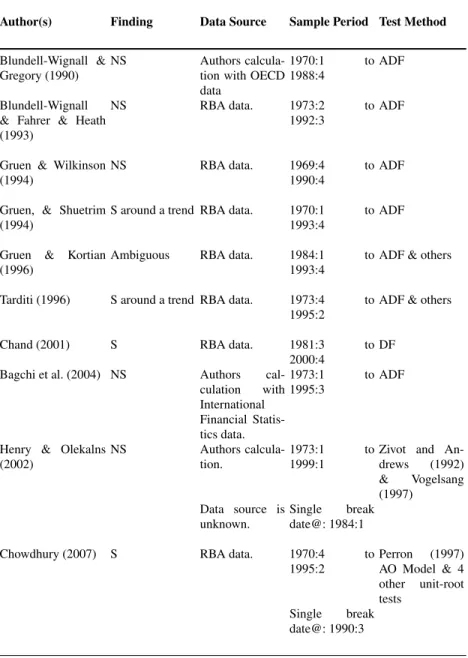
This shallow evidence in the Australian literature highlights the difficulties of detecting robust evidence in favour of, or against, the PPP theory . A summary of past results is given in Table 1 for a ready reference. Therefore, further research is warranted to determine if PPP provides a valid representation of the long-run equilibrium relation between the exchange rate and relative prices in Australia by exploring the possibility of including multiple structural breaks. The next section is devoted to this particular aspect.
3 Time-series properties of RER in the presence of structural
breaks
3.1 Data and data source
We performed the LS minimum Lagrange Multiplier (LM) unit-root tests to de-termine structural breaks endogenously. The LS unit-root test with two structural breaks endogenously determines the location of two breaks in level and trend and tests the null of a unit-root. The LS unit-root test with two structural breaks is invari-ant to the magnitude of the breaks. LS noted that the alternative of the minimum LM unit-root test with two structural breaks unambiguously implies trend stationarity; however, it could be true that the series can possess unit-root with structural breaks. Unit-root tests for one (LS1) and two breaks (LS2) were conducted with RATS 7.2. We estimated two models: Break Model and Crash Model. The LS-Break Model captures the change that is gradual whereas LS-Crash Model picks up the change that is rapid. We have reported the results of both models in Table 2 which are contradictory to each other. The result of the unit-root test is contingent
Table 1 Summary of Previous Results of Unit-root in the Australian RER
Author(s) Finding Data Source Sample Period Test Method
Blundell-Wignall & Gregory (1990)
NS Authors calcula-tion with OECD data
1970:1 to 1988:4
ADF
Blundell-Wignall & Fahrer & Heath (1993)
NS RBA data. 1973:2 to 1992:3
ADF
Gruen & Wilkinson (1994)
NS RBA data. 1969:4 to 1990:4
ADF
Gruen, & Shuetrim (1994)
S around a trend RBA data. 1970:1 to 1993:4
ADF
Gruen & Kortian (1996)
Ambiguous RBA data. 1984:1 to 1993:4
ADF & others
Tarditi (1996) S around a trend RBA data. 1973:4 to 1995:2
ADF & others
Chand (2001) S RBA data. 1981:3 to 2000:4
DF Bagchi et al. (2004) NS Authors
cal-culation with International Financial Statis-tics data. 1973:1 to 1995:3 ADF
Henry & Olekalns (2002)
NS Authors calcula-tion.
1973:1 to 1999:1
Zivot and An-drews (1992) & Vogelsang (1997) Data source is unknown. Single break date@: 1984:1 Chowdhury (2007) S RBA data. 1970:4 to
1995:2 Perron (1997) AO Model & 4 other unit-root tests Single break date@: 1990:3
Note: S = Stationary; NS = Non-stationary; @=Assume no break under the null hypothesis of unit root.
upon the way the breaks are modelled. The choice of the “modelshould be based on economic theory and reality. Based on our judgement, we think the LS Trend Break model is the optimal model to discuss.
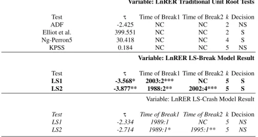
On the basis of LS1unit-root test we find LnRER to be stationary. By applying the LS2 unit-root test we found that LnRER is also stationary. Rejection of the unit-root null provides evidence of mean reversion and hence PPP.
Table 2 Unit-Root Tests in the Absence and Presence of Structural Breaks
Variable: LnRER Traditional Unit Root Tests
Test τ Time of Break1 Time of Break2 kDecision
ADF -2.425 NC NC 2 NS
Elliot et al. 399.551 NC NC 2 S
Ng-Perron5 30.418 NC NC 4 S
KPSS 0.184 NC NC 5 NS
Variable: LnRER LS-Break Model Result
Test τ Time of Break1 Time of Break2 kDecision
LS1 -3.568* 2003:2*** NC 5 S LS2 -3.877** 1988:2** 2002:4*** 5 S
Variable: LnRER LS-Crash Model Result
Test τ Time of Break1 Time of Break2 kDecision
LS1 -2.334 1989:1 NC 5 NS
LS2 -2.714 1989:1* 1995:1** 5 NS
Note:aNC = Not calculated; S = Stationary, NS = Nonstationary.bt-statistic for the null hypoth-esis =0.c ADF Test critical values at 1, 5 and 10 per cent level are -4.054; -3.456 and -3.153 respectively. d Critical values of the endogenous two-break LM unit-root test at 10%, 5% and 1% level of significance are -3.504, -3.842 and -4.545 respectively from Table 2 Lee and Strazicich (2003:1084).e We report the first unit root test statistic developed by Ng and Perron which is the Elliot, Rothenberg, and Stock (1996) point optimal statistic for GLS de-trended data. The other three statistics, , and are the enhancements of the Phillips-Peron (PP) test statistics, which are not reported here. f (*), (**) and (***) refer to significant at 10, 5 and 1 per cent level of significance respectively.
ADF test fails to reject the null hypothesis for LnRER (refer to Table 2). The GLS test proposed by Elliotet al.(1996) and M ˜test suggested by Ng and Perron (2001) reject the null of a unit-root for LnRER. However, based on the KPSS test we reject the null hypothesis of stationarity for LnRER. On balance, the evidence in Table 2 is inconclusive.
3.2 Lee and Strazicich (2003) (LS) unit-root test
We performed the LS minimum Lagrange Multiplier (LM) unit-root tests to de-termine structural breaks endogenously. The LS unit-root test with two structural
breaks endogenously determines the location of two breaks in level and trend and tests the null of a unit-root. The LS unit-root test with two structural breaks is invari-ant to the magnitude of the breaks. LS noted that the alternative of the minimum LM unit-root test with two structural breaks unambiguously implies trend stationarity; however, it could be true that the series can possess unit-root with structural breaks. Unit-root tests for one (LS1) and two breaks (LS2) were conducted with RATS 7.2. We estimated two models: Break Model and Crash Model. The LS-Break Model captures the change that is gradual whereas LS-Crash Model picks up the change that is rapid. We have reported the results of both models in Table 2 which are contradictory to each other. The result of the unit-root test is contingent upon the way the breaks are modelled. The choice of the ?best model? should be based on economic theory and reality. Based on our judgement, we think the LS Trend Break model is the optimal model to discuss.
On the basis of LS1unit-root test we find LnRER to be stationary. By applying the LS2 unit-root test we found that LnRER is also stationary. Rejection of the unit-root null provides evidence of mean reversion and hence PPP.
3.3 Endogenously Determined Structural Break Dates
The estimated single structural break date determined by the LS1 Break Model cor-responds to 2003 quarter 2 for LnRER. The break date is statistically significant at the 5 per cent level. By considering the two breaks LS2 Trend Break Model, the corresponding break dates for LnRER are 1988:2 and 2002:4. The structural break dates are all statistically significant. The first break date of LnRER coincides with the abandonment of the ?check-list? approach in favour of ?discretionary? approach to monetary policy by RBA in 1988 quarter 2. This structural break may also be capturing the effect of the stock market crash of October 1987, and the onset of recession at the end of the 1980s culminating into the recession in 1990. The be-haviour of the Australian RER shows periods of instability. One such period was centred around June 1986, the other between March 1998 and June 1999. After a sustained period of depreciation, appreciations of the RER occurred during 1986-1989 so that the break date for the RER is picked up in 1988 quarter 2 followed by the meltdown in 2001 and again a recovery in early 2002. The second break date is found to be in 2002 quarter 4 which is due to the sudden appreciation of the Australian dollar. Between January 2002 and July 2008, the Australian dollar appreciated sharply from 51 US cents to 97 US cents which was largely driven by increased demand for Australian exports.
4 Summary and Conclusion
We investigate evidence of mean reversion in the Australian dollar RER. Conven-tional unit-root tests fail to provide evidence of stationarity of RER. If RER is non-stationary, then PPP is no longer valid as a representation of the long-run equi-librium relation between the exchange rate and relative prices. The conventional unit-root tests may suffer from severe size distortions and results might be erro-neous since they do not account for structural breaks in the data. To overcome the loss of power in conventional unit-root tests, we performed the LS (2003) minimum Lagrange Multiplier unit-root tests in the presence of structural breaks.
Based on our result, we were able to reject the unit-root null hypothesis and find evidence of mean reversion and hence PPP. This result is consistent with Chowd-hury’s (2007) finding although the break dates are different. This finding reverses the findings of past works that failed to reject non-stationarity. The corresponding break dates for RER are 1988 quarter 2 and 2002 quarter 4 respectively; and the break dates are all statistically significant. The estimated break dates mostly correspond to the period of RER instability (1986-1989) and the recovery of the Australian dollar driven by the resources boom (2001-2002).
Appendix
A Brief Review of Unit-root Tests
9Traditional (First Generation Models) tests for unit-roots (such as Dickey-Fuller, Augmented Dickey-Fuller and Phillips-Perron) have low power in the presence of structural break. Perron (1989) demonstrated that, in the presence of a structural break in time-series, many perceived non-stationary series were in fact stationary. Perron (1989) re-examined Nelson and Plosser (1982) data and found that 11 of the 14 important US macroeconomic variables were stationary when known exogenous structural break is included10. Perron (1989) allows for a one time structural change occurring at a time TB(1<TB<T), where T is the number of observations.
The following models were developed by Perron (1989) for three different cases. Notations used in equations A1- A16 are the same as in the papers quoted. Null Hypothesis:
Model(A)yt=µ+dD(T B)t+yt−1+et (2)
Model(B)yt=µt+yt−1+ (µ2−µ1)DUt+et (3)
9The discussion that follows is for reference only and may be omitted.
10However, subsequent studies using endogenous breaks have countered this finding with Zivot
Model(C)yt=µt+yt−1+dD(T B)t+ (µ2−µ1)DUt+et (4) WhereD(T B)t=1i f t=TB+1,0 otherwise, and DUt=1i f t>TB,0 other-wise.
Alternative Hypothesis:
Model(A)yt=µt+βt+ (µ2−µ1)DUt+et (5)
Model(B)yt=µ+βtt+ (β2−β1)DTt∗+et (6)
Model(C)yt=µ+β1t+ (µ2−µ1)DUt+ (β2−β1)DTt+et (7) WhereDTt∗=t−TB, i f t>TB, and O otherwise.
Model A permits an exogenous change in the level of the series whereas Model B permits an exogenous change in the rate of growth. Model C allows change in both. Perron (1989) models include one known structural break. These models cannot be applied where such breaks are unknown. Therefore, this procedure is criticised for assuming known break date which raises the problem of pre-testing and data mining regarding the choice of the break date (Maddala and Kim 2003). Further, the choice of the break date can be viewed as being correlated with the data.
Second Generation Models
Unit-Root Tests in the Presence of a Single Endogenous Structural Break
Despite the limitations of Perron (1989) models, they form the foundation of sub-sequent studies that we are going to discuss hereafter. Zivot and Andrews (1992), Perron and Vogelsang (1992), and Perron (1997) among others have developed unit-root test methods which include one endogenously determined structural break. Here we review these models briefly and detailed discussions are found in the cited works. Zivot and Andrews (ZA) (1992) models are as follows:
Model with Intercept
yt=µˆA+θˆADUt(λˆ) +βˆAt+αˆAyt−1+ k
∑
j=14cˆAjyt−j+eˆt (8)
Model with Trend
yt=µˆB+βˆBt+γˆBDT∗t(λˆ) +αˆBYt−1+ k
∑
j=1 ˆ cBj4yt−j+eˆt (9)Model with Both Intercept and Trend yt=µˆC+θˆCDUt(λˆ) +βˆct+γˆcDTt∗(λˆ) +αˆcyt−1+ k
∑
j=1 ˆ cCj 4yt−j+eˆt (10) Where,DUt(α) =1 i f t>T{α,0 otherwise;DTt∗(λ) =t−Tλ i f t >Tλ, 0 otherwise.The above models are based on Perron (1989) models. However, these modified models do not include DTb.
On the other hand, Perron and Vogelsang (PV) (1992) include DTb but exclude t in their models. PV (1992) models are given below:
Innovational Outlier Model (IOM)
yt=µ+δDUt+θD(Tb)t+αyt−1+ k
∑
j=1 ˆ cCj4yt−j+eˆt (11)Additive Outlier Model (AOM)? Two Steps
yt=µ+δDUt+y˜t (12) and ˜ yt= k
∑
j=0 wtD(Tb)t−1+αy˜t−1+ k∑
j=1 cj4y˜t−j+et (13) ˜yin the above equations represents a detrended series y. Perron (1997) includes both t (time trend) andDTb(time at which structural change occurs) in his Innova-tional Outlier (IO1 and IO2) and Additive Outlier (AO) models. InnovaInnova-tional Outlier Model allowing one time change in intercept only (IO1):
yt=µ+θDUt+βt+γD(Tb)t+αyt−1+ k
∑
j=1ci4yt−j+et (14)
Innovational Outlier Model allowing one time change in both intercept and slope (IO2): yt=µ+θDUt+βt+γD(Tb)t+γD(Tb)t+αyt−1+ k
∑
j=1 ci4yt−j+et (15)Additive Outlier Model allowing one time change in slope (AO):
yt=µ+βt+γDTt∗+y˜t (16) whereDTt∗=1(t>Tb)(t−Tb) ˜ yt=αy˜t−1+ k
∑
j=1 ˆ cCj4y˜t−j+et (17)The Innovational Outlier models represent the change that is gradual whereas Additive Outlier model represents the change that is rapid.
Regarding the power of tests, the PV (1992) model is robust. The testing power of Perron (1997) and ZA (1992) models are almost the same. On the other hand, Perron (1997) model is more comprehensive than ZA (1992) model as the former includes both t and DTb while the latter includes t only.
Additional test methods have been proposed for unit-root test allowing for mul-tiple structural breaks in the data (Lumsdaine and Papell (LP) 1997; Lee and Strazi-cich (LS) 2003). One important issue common to the ZA and LP (and other similar) endogenous break tests is that they assume no break(s) under the unit-root null and derive their critical values accordingly. Thus, the alternative hypothesis would be ?structural breaks are present,? which includes the possibility of a unit-root with break(s). Thus, rejection of the null does not necessarily imply rejection of a unit-root per se, but would imply rejection of a unit-unit-root without breaks.
Third Generation Models
Lee and Strazicich (LS) (2003) Minimum LM Unit-Root Test
LS propose a minimum Lagrange multiplier (LM) unit-root test in which the alternative hypothesis unambiguously implies trend stationarity. Consider the DGP as follows:
4yt=δ0+4Zt+φS˜t−1+ut (18) where ˜St=yt−ψ˜x−Ztδ˜(t=2, . . .T and is a vector of exogenous variables defined
by the data generating process; ˜δis the vector of coefficients in the regression of4yt on4Zt respectively with4 the difference operator; and ˆψx=y1−Z1δ˜, withy1 andZ1the first observations ofyt andZtrespectively.
Model B of Perron (1989) is omitted by LS (2003), as it is commonly held that most economic time-series can be adequately described by model A or C. Equivalent to Perron?s (1989) Model C, which allows for a shift in intercept and change in trend slope under the null hypothesis and is described asZt= [1,t,Dt,DTt]0, where DTt=t−TBfort>TB+1, fort>T B+1, and zero otherwise. It is important to note here that testing regression (18) involves using4Zt instead ofZt.4Ztis described by [1, BtDt]0whereBt =4Dt andDt =4DTt . Thus,Bt andDt correspond to a change in the intercept and trend under the alternative and to a one period jump and (permanent) change in drift under the null hypothesis, respectively.
The unit-root null hypothesis is described in (18) byφ=0 and the LM t-test is
˜
τ=tgiven by ; where ˜τ=t−statisticfor the null hypothesisφ=0.
The augmented terms4St˜−j,j=1, ...k,terms are included to correct for serial correlation. The value of k is determined by the general to specific search procedure. General to specific procedure begins with the maximum number of lagged first dif-ferenced terms max k =8 and then examine the last term to see if it is significantly
different from zero. If insignificant, the maximum lagged term is dropped and then estimated at k =7 terms and so on, till the maximum is found ork=0. To endoge-nously determine the location of the break(TB), the LM unit-root searches for all possible break points for the minimum (the most negative) unit-root t -test statistic as follows:
In fτ˜=in fλτ˜(λ);whereλ=TB/T. (19) The two-break LM unit-root test statistic can be estimated analogously. Critical values of the two-break LM unit-root test (T = 100) is reported in Table 3 by LS. LS (2003: 1087) conclude “summary, the two-break minimum LM unit-root test pro-vides a remedy for a limitation of the two-break minimum LP test that includes the possibility of a unit-root with break(s) in the alternative hypothesis. Using the two-break minimum LM unit-root test, rejection of the null hypothesis unambiguously implies trend stationarity.”
References
1. Bagchi B, Chortareas GE, Miller SM. (2004) The Real Exchange Rate in Small, Open Devel-oped Economies: Evidence from Cointegration Analysis. Economic Record, 80(248). 76-88. 2. Baum CF, Barkoulas JT, Caglayan M (2001) Nonlinear Adjustment to Purchasing Power Parity in the Post-Bretton Woods Era, Journal of International Money and Finance, 20, 379-399.
3. Blundell-Wignall A, Fahrer J, Heath A.(1993) Major Influences on the Australian Dollar Exchange Rate, in A. Blundell-Wignall (ed), The Exchange Rate, International Trade and the Balance of Payments, Proceedings of a Conference, Reserve Bank of Australia, 30-78. 4. Blundell-Wignall A, Gregory RG (1990) Exchange Rate Policy in Advanced
Commod-ity Exporting Countries: Australia and New Zealand, ”Exchange Rate Policy in Advanced Commodity-Exporting Countries: The Case of Australia and New Zealand”, OECD Eco-nomics Department Working Papers, No. 83.
5. Chand S (2001) How Misaligned is the Australian Real Exchange Rate?, Working Paper Number 012, Asia Pacific School of Economics and Government, Australian National Uni-versity, Canberra.
6. Chowdhury K (2007) Are the Real Exchange Rate Indices of Australia Non-Stationary in the Presence of Structural Break? International Review of Business Research Papers, 3 (5), 161-181.
7. Corbae D,Ouliaris S (1990) A Test of Long-Run Purchasing Power Parity Allowing for Struc-tural Breaks, The Economic Record, 67, 26-33.
8. Cuestas JC, Gil-Alana LA (2009) Further Evidence on the PPP Analysis of the Australian Dollar: Non-Linearities, Fractional Integration and Structural Changes Economic Modelling, 26, 1184-1192.
9. Cuestas JC, Regis JC (2008) Testing for PPP in Australia: Evidence from Unit Root Tests against Nonlinear Trend Stationarity Alternatives, Economics Bulletin, 27, 1-8
10. Darn O, Hoarau JF (2008) The Purchasing Power Parity in Australia: Evidence from Unit Root Test with Structural Break, Applied Economics Letters, 15, 203-206.
11. Dornbusch R (1976) Expectations and Exchange Rate Dynamics, Journal of Political Econ-omy, 84, 1161-1176.
12. Edison H, Cashin P, Liang H (1999) Foreign Exchange Intervention and the Australian Dollar: Has it Mattered? IMF Working Paper, WP/03/99.
13. Elliot G, Rothenberg TJ, Stock JH (1996), Efficient Tests for an Autoregressive Unit Root, Econometrica, 64, 813-836.
14. Ellis L (2001) Measuring the Real Exchange Rate: Pitfalls and Practicalities Research Dis-cussion Paper 2001-04, Economic Research Department, Reserve Bank of Australia. 15. Frenkel JA (1981) The Collapse of Purchasing Power Parities during the 1970s, European
Economic Review, 16, 145-165.
16. Granger CWJ, Terasvirta T (1993) Modelling Nonlinear Economic Relationships, Oxford University Press, Oxford.
17. Gruen DWR, Wilkinson J (1994) Australias Real Exchange Rate Is It Explained by the Terms of Trade or by Real Interest Rate Differential?, The Economic Record, 70, 204–219. 18. Gruen DWR, Kortian T (1996) Why does the Australian Dollar Move with the Terms of
Trade? Research Discussion Paper 9601, Economic Group, Reserve Bank of Australia. 19. Gruen DWR, Shuetrim G (1994) Internationalisation and the Macroeconomy, in P. Lowe
and J. Dwyer (eds), International Integration of the Australian Economy, Proceedings of a Conference, Reserve Bank of Australia, Sydney, 309-363.
20. Henry OT, Olekalns N (2002) Does the Australian Dollar Real Exchange Rate Display Mean Reversion, Journal of International Money and Finance, 21, 651-666.
21. Henry OT, Olekalns N, Summers PM(2001) Exchange Rate Instability: A Threshold Autore-gressive Approach, The Economic Record, 77, 160-166.
22. Kwiatkowski D, Phillips PCB, Schmidt P, Shin Y(1992) Testing the Null Hypothesis of Sta-tionarity against the Alternative of a Unit Root, Journal of Econometrics, 55, 159-178. 23. Jones MT, Wilkinson J (1990) Real Exchange Rates and Australian Export Competitiveness,
Discussion Paper No. 9005, Economics Research Department, Reserve Bank of Australia. 24. Lee J, Strazicich M (2003) Minimum Lagrange Multiplier Unit Root Test with Two Structural
Breaks, The Review of Economics and Statistics, 85(4), 1082-1089.
25. Lee J, Strazicich M (2001) Break Point Estimation and Spurious Rejections with Endogenous Unit Root Tests, Oxford Bulletin of Economics and Statistics, 63(5), 535-558.
26. Liew KS, Baharumshah AZ, Lau E, (2004) Nonlinear Adjustment Towards Purchasing Power Parity in ASEAN Exchange Rates, International Journal of Applied Economics, 3(6), 7-18. 27. Lumsdaine R, Papel DH (1997) Multiple Trend Breaks and the Unit Root Hypothesis, Review
of Economics and Statistics, 79, 212-218.
28. Maddala GS, Kim IM (2003) Unit Roots, Cointegration, and Structural Change, Cambridge University Press, Cambridge.
29. MacDonald R (1996) Panel Unit Root Tests and Real Exchange Rates, Economic Letters, 50, 7-11.
30. Michael P, Nobay AR, Peel DA (1997) Transaction Costs and Nonlinear Adjustment in Real Exchange Rates: An Empirical Investigation, Journal of Political Economy, 105, 862-879. 31. Ng S, Perron P (2001), Lag Length Selection and the Construction of Unit Root Tests with
Good Size and Power, Econometrica, 69, 1519-1554.
32. Nelson C, Plosser C (1982) Trends and Random Walks in Macroeconomic Time Series: Some Evidence and Implications, Journal of Monetary Economics, 10, 139-162.
33. Olekalns N, Wilkins N (1998) Re-examining the Evidence for Long-Run Purchasing Power Parity, The Economic Record, 74, 54–61
34. Papell D (1997) Searching For Stationarity: Purchasing Power Parity under the Current Float, Journal of International Economics, 43, 313-332.
35. Papell D, Theodoridis H (2001) The Choice Of Numeraire Currency in Panel Tests of Pur-chasing Power Parity, Journal of Money, Credit, and Banking, 33, 790-803.
36. Papell D, Theodoridis H (1998) Increasing Evidence of Purchasing Power Parity over the Current Float, Journal of International Money and Finance, 17(1), 41-50.
37. Perron P (1989) The Great Crash, the Oil Price Shock, and the Unit Root Hypothesis, Econo-metrica, 57, 1361-1401.
38. Perron P (1997) Further Evidence on Breaking Trend Functions in Macroeconomic Variables, Journal of Econometrics, 80, 355-385.
39. Perron P, Vogelsang TJ (1992) Nonstationary and Level Shifts with an Application to Pur-chasing Power Parity, Journal of Business and Economic Statistics, 10, 301-320.
40. Phillips PCB, Perron P (1988) Testing for a Unit Root in Time Series Regression, Biometrica, 75, 335-346.
41. Sarno L (2000a) Real Exchange Rate Behaviour in High Inflation Countries: Empirical Evi-dence From Turkey, 1980-1997, Applied Economics Letters, 7, 285291.
42. Sarno L (2000b) Real Exchange Rate Behaviour in the Middle East: A Re-Examination, Economics Letters, 66, 127-136.
43. Shrestha MB, Chowdhury K (2005) A Sequential Procedure for Testing Unit Roots in the Presence of Structural Break in Time Series Data: An Application to Quarterly Data in Nepal, 19702003, International Journal of Applied Econometrics and Quantitative Studies, 2(2), 1-16.
44. Tarditi A(1996) Modelling the Australian Exchange Rate, Long Bond Yield and Inflation-ary Expectations, Research Discussion Paper 9608, Economic Analysis Department, Reserve Bank of Australia.
45. Taylor M P, Peel DA(2000) Nonlinear Adjustment, Long-Run Equilibrium and Exchange Rate Fundamentals, Journal of International Money and Finance, 19, 33-53.
46. Vogelsang TJ (1997) Wald-Type Test for Detecting Breaks in the Trend Function of a Dy-namic Time Series, Econometric Theory, 13, 818-849.
47. Zivot E, Andrews DW(1992) Further Evidence on the Great Crash, the Oil-Price Shock, and the Unit-Root Hypotheses, Journal of Business and Economic Statistics, 10, 251-270.