Variable Selection in Additive Models
by Nonnegative Garrote
Eva Cantoni, Joanna Mills Flemming
and Elvezio Ronchetti
No 2006.02
Cahiers du département d’économétrie
Faculté des sciences économiques et sociales
Université de Genève
Mars 2006
Département d’économétrie
Université de Genève, 40 Boulevard du Pont-d’Arve, CH -1211 Genève 4
Variable Selection in Additive Models
by Nonnegative Garrote
Eva Cantoni
◦, Joanna Mills Flemming
∗, Elvezio Ronchetti
◦◦
Department of Econometrics
University of Geneva
1211 Geneva 4, Switzerland
∗
Department of Mathematics and Statistics
Dalhousie University
Halifax, Nova Scotia, Canada B3H 4J1
[email protected], [email protected]
,
[email protected]
Abstract
We adapt Breiman’s (1995) nonnegative garrote method to per-form variable selection in nonparametric additive models. The tech-nique avoids methods of testing for which no reliable distributional theory is available. In addition it removes the need for a full search of all possible models, something which is computationally intensive, especially when the number of variables is moderate to high. The method has the advantages of being conceptually simple and com-putationally fast. It provides accurate predictions and is effective at identifying the variables generating the model. For illustration, we consider both a study of Boston housing prices as well as two simula-tion settings. In all cases our methods perform as well or better than available alternatives like the Component Selection and Smoothing Operator (COSSO).
Keywords: cross-validation; nonnegative garrote; nonparametric regres-sion; shrinkage methods; variable selection.
1
Introduction
Variable selection is an important issue in any statistical analysis, whether parametric or nonparametric in nature. Practically speaking, one is inter-ested in determining the strongest effects that explain the response variable. Statistically speaking, variable selection is a way of reducing the complexity of the model, in some cases by admitting a small amount of bias to improve accuracy. For example, consider the study of the Boston Housing Data (avail-able from the University of California at Irvine Repository Of Machine
Learn-ing Database at http://www.ics.uci.edu/~mlearn/MLRepository.html,
aimed at describing the relationship between housing values in suburbs of Boston and different attributes as shown in Table 1. The data (originally from Harrison and Rubinfeld, 1978) have been considered by Belsley, Kuh, and Welsch (1980), among others, with various transformations proposed for the predictors. These data are therefore a good candidate with which to illustrate a nonparametric regression approach. The sample size is 506.
The full model (containing all available explanatory variables) for the Boston Housing Data can be written as:
log(medv) = α+f1(crim) +f2(zn) +f3(indus) +f4(nox) +f5(rm) + f6(age) +f7(dis) +f8(rad) +f9(tax) +f10(ptratio) + f11(b) +f12(lstat) +βchas+. (1)
Note that chas is a dummy variable and consequently does not require
any smoothing. Also, we could have chosen to use Bk, where Bk is the
proportion of blacks by town, rather than b = 1000(Bk−.63)2 due to the
nonparametric nature of the analysis but instead elected to remain consistent with the original analysis in this regard. These data are analyzed in Section 2. A nonparametric framework is more challenging than a parametric ap-proach because of the lack of underlying assumptions that makes it difficult to define a general test approach for variable selection. Some notable exceptions exist, but only with strong restrictions: in special situations or for particular smoothers (see, e.g. Bock and Bowman, 1999 for local polynomials; Cantoni and Hastie, 2002 for smoothing splines).
Subset selection is a well-known approach to variable selection: it selects a model containing a subset of available variables, according to a given opti-mality criterion and requires that one visit all possible models. This approach quickly becomes infeasible when the dimension is too large even when
effi-cient algorithms exist (e.g. leaps and bounds in the case of linear regression,
see Furnival and Wilson, 1974). Stepwise procedures are a working compro-mise as they reduce the number of models for comparison. However, they
medv median value of owner occupied homes in $1000’s
crim per capita crime rate by town
zn proportion of residential land zoned for lots over 25,000 sq.ft.
indus proportion of non-retail business acres per town
nox nitric oxides concentration (parts per 10 million)
rm average number of rooms per dwelling
age proportion of owner-occupied units built prior to 1940
dis weighted distances to five Boston employment centres
rad index accessibility to radial highways
tax full-value property-tax rate per $10,000
ptratio pupil-teacher ratio by town
b 1000(Bk−0.63)2 where Bk is the proportion of blacks by town
lstat proportion of the population that is lower status
chas Charles River dummy variable (=1 if tract bounds river; 0 otherwise)
Table 1: Boston Housing Data description.
suffer from dependence on the path chosen through the variable space and may be inconsistent. In addition, both subset selection and stepwise selection are discrete processes that either retain or discard one variable and therefore shrinkage methods (e.g. ridge regression in the case of linear models) should be preferred because of their continuity in this regard, which leads to lower variability.
Shrinkage methods have emerged and gained popularity (especially in the parametric context) in recent years. In addition, methods that simultane-ously address estimation and variable selection now exist (e.g. LASSO, see Tibshirani, 1996, and LARS, see Efron, Hastie, Johnstone, and Tibshirani, 2004). In the nonparametric setting, the method of COSSO has been pro-posed by Lin and Zhang (2003). It applies to the smoothing splines ANOVA framework as defined in Gu (2002). Efficient algorithms for model selection with shrinkage methods have been provided by Yuan and Lin (2006).
In this paper, we propose an approach to variable selection for nonpara-metric additive models based on the nonnegative garrote idea of Breiman (1995) which has simultaneously the properties of subset selection, shrinkage and stability as mentioned above. It also has the advantage of being concep-tually simple (like its original parametric counterpart) and computationally cheap. Moreover, it can be used with any smoother. These desirable charac-teristics are not shared by alternative methods like COSSO with which we compare results.
and is able to identify the true underlying model, with the procedure (C) (see Section 2.1) giving the best results in general. This is true when compared to COSSO as well as stepwise procedures.
The paper is organized as follows. We introduce the methodology in Section 2. Specifically, we discuss the automatic choice of the parameters involved (Sections 2.1 and 2.2) and provide guidelines for different options. In the same section we present an illustrative example, followed by results of a simulation study in Section 3. Both demonstrations provide strong evidence that our proposal works well under a variety of circumstances. A discussion (Section 4) closes the paper.
2
Methodology
A typical dataset of interest here will consist of p explanatory variables
x1i, . . . , xpiand a response variableYifor each of thei= 1, . . . , nindependent
individuals for which we postulate an additive model of the form
Yi =α+ p X k=1 fk(xki) +i, (2) for i= 1, . . . , n.
Model (2) is often presented with only univariate functions for conve-nience, but it must be emphasized that this property is not necessary. In fact, component functions with two or more dimensions, as well as categor-ical variable terms (factors) and interactions between them can replace the
univariate functions fk(xk). Moreover, some of the functions in Model (2)
may be defined parametrically, giving rise to a semiparametric model.
We suppose that the variables xk have been centered by subtracting off
their sample means. This is not a theoretical restriction, but rather for ease of implementation, see Section 2.3 for further details.
Given an initial estimate ˆghk
k (xk) of each functionfk(xk), the nonnegative
garrote approach solves min ck n X i=1 yi−α− p X k=1 ckgˆkhk(xki) 2 (3)
under the constraints ck ≥0 and
Pp
k=1ck ≤s. The final estimate of fk(xki)
is ˆfk(xki) =ckgˆkhk(xki).
The set h1, . . . , hp are referred to as the smoothing parameters of the
initial function estimates ˆgh1
1 , . . . ,ˆg
hp
0 5 10 15 0.0 0.5 1.0 1.5 2.0 2.5 s ck chas crim zn indus nox rm age dis rad tax ptratio b lstat
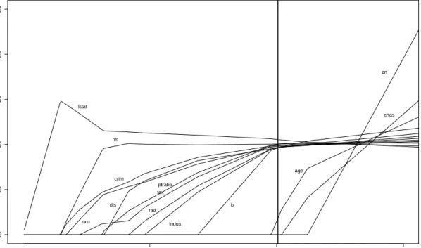
Figure 1: Shrinkage values ck as a function of s for the Boston Housing
data. The bold vertical line indicates the value of s chosen by 5-fold
cross-validation.
degrees of freedom (see Hastie and Tibshirani, 1990, p. 128). Most smoothing techniques (e.g. splines, loess, local polynomials), allow one parameter for each function [the AMlet technique (Sardy and Tseng, 2004) is an exception
here in that it requires only a single parameter]. Note also that ck depends
ons, andsis regarded as an additional parameter. We will discuss the choice
of these parameters in Sections 2.1 and 2.2 below.
Our proposal (3) generalizes the original proposal of Breiman (1995)
which is recovered with ˆghk
k (xk) = ˆβkxki, where ˆβk are the ordinary least
square estimates in the linear model yi =α+
Pp
k=1βkxki+i. In this
para-metric situation no choice of h1, . . . , hp is required.
Given an initial estimate of all the additive functions in Model (2) and
a value for s, the nonnegative garrote will automatically and in a single
step provide a set of coefficients c1, . . . , cp that will provide information on
the importance of each variable in the model. For instance, if ck = 0, the
variable xk is considered uninformative and can be removed from the model.
proportion ck or left unchanged (if ck = 1). Decreasing s has the effect of
increasing the shrinkage of the nonzeroed functions and making more of the
ck become zero. The nonnegative garrote can be viewed as a method for
comparing all possible models, but unlike subset selection, it avoids fitting each model separately, therefore making its use possible at low computational
cost even for large values of p.
For example, if we apply our proposal to the Boston Housing data (on log
scale, see Equation (1)) with smoothing parameters h1, . . . , hp automatically
chosen according to Procedure (C) (see Section 2.1 below), we obtain the results as depicted in Figure 1. This plot identifies the strongest effects (the
components that enter first in the model assincreases) which in this case are
lstat,crimandrm. The bold vertical line shows the value ofsautomatically
chosen by 5-fold cross-validation (see Section 2.2). Thoseckwhich are zero for
this value of s (=10.05) identify the variables that can be removed from the
final model: znandchas. The significance ofageis borderline. Although the
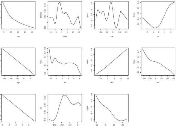
model considered here is different, the conclusions are partly common with those of Belsley, Kuh, and Welsch (1980). Furthermore, the nonparametric model considered in our analysis is certainly a welcome alternative to their linear analysis given the strong nonlinear effects observed when the final model is plotted as shown in Figure 2.
2.1
Choice of
h
1, . . . , h
pIn order for the method to perform well, it is important that the smoothing
parametersh1, . . . , hpof the initial fits ˆgkhk be selected in a reasonable manner.
They can either be set by the user (maybe on the basis of asymptotic results as in the plug-in approach) or selected automatically with a data driven ap-proach (e.g. cross-validation); see, for example, H¨ardle (1990, Chapter 5). Note that until the recent contribution of Wood (2000), no satisfactory solu-tion to the problem of automatic selecsolu-tion of the smoothing parameter has been available.
In our work, we will consider the following non exhaustive list of options with which to obtain an initial fit of the data:
(A) Estimateh1, . . . , hp automatically (by cross-validation, for example) on
the basis of the punivariate nonparametric regressions yi =gk(xki) +i
for k = 1, . . . , p, to produce ˆghk
k .
(B) Given starting valuesh0
1, . . . , h0pprovided by the user, estimateh1, . . . , hp
automatically (by cross-validation, for example) at each step of the backfitting algorithm (Hastie and Tibshirani, 1990, p. 91). This modi-fied backfitting algorithm reads as follows:
0 20 40 60 80 −0.6 −0.4 −0.2 0.0 crim f(crim) −10 −5 0 5 10 15 −0.10 0.00 0.05 0.10 indus f(indus) −0.1 0.0 0.1 0.2 0.3 −0.2 −0.1 0.0 0.1 0.2 nox f(nox) −2 −1 0 1 2 0.0 0.1 0.2 0.3 0.4 rm f(rm) −60 −40 −20 0 20 −0.002 0.002 0.006 age f(age) −2 0 2 4 6 8 −0.3 −0.1 0.1 0.2 0.3 dis f(dis) −5 0 5 10 15 −0.1 0.0 0.1 0.2 0.3 rad f(rad) −200 −100 0 100 200 300 −0.2 −0.1 0.0 0.1 0.2 tax f(tax) −6 −4 −2 0 2 −0.10 0.00 0.10 0.20 ptratio f(ptratio) −300 −200 −100 0 −0.10 −0.05 0.00 0.05 b f(b) −10 0 10 20 −0.4 −0.2 0.0 0.2 0.4 lstat f(lstat)
Figure 2: Fitted functions for the final model after variable selection by our nonparametric nonnegative garrote.
1. Initialize: ˆα = ¯y, hk = h0k for k = 1, . . . , p, and ˆg hk k = ˆg h0 k k for k = 1, . . . , p. 2. Cycle: j = 1, . . . , p,1, . . . , p, . . . Produce estimates ˆghj
j by smoothing the partial residuals Yi −
ˆ
α−Pk6=jgˆhk
k (xki)
onxj, with hj chosen automatically.
3. Continue Step 2 until the individual functions do not change.
(C) Estimate h1, . . . , hp automatically by minimizing a given criterion in
the p dimensional space.
Procedure (C) is certainly the most desirable, but is not yet widely im-plemented in software packages. Procedure (A) is the simplest approach but neglects the correlation between covariates. Procedure (B) is a working com-promise but is again effective only when there is little covariance between covariates. Note that the re-estimation of the smoothing parameter at each step of the backfitting algorithm might, in principle, affect the convergence of the backfitting algorithm. However, we never experienced this situation in our examples and simulations. We can expect procedure (C) to perform better than (B), which in turn would perform better than (A), but it is not clear a priori how large the differences will be.
2.2
Choice of
s
The accuracy of the model can be measured through the (average) prediction error defined as P Es( ˆα,fˆh 1 1 (x1i), . . . ,fˆphp(xpi)) = 1 n n X i=1 EYinew−αˆ− p X k=1 ˆ fhk k (xki) 2 , (4)
where s = Ppk=1ck, ˆfkhk(xki) = ckgˆkhk(xki) and the expectation on the right
hand side of (4) is taken over Ynew
i . The best value of s is then defined as
the minimizer of P Es( ˆα,fˆ1h1(x1i), . . . ,fˆ hp p (xpi)). Of course, in practiceP Es( ˆα,fˆh 1 1 (x1i), . . . ,fˆ hp
p (xpi)) is not observable and
needs to be estimated. V-fold cross-validation is an approach used to mimic
the behaviour of new observations coming into play, when only a single
sam-ple is available. It splits the data into V subsets. Denote by I1, . . . ,IV
the sets of the corresponding observation indices. For each value of s, the
cross-validation estimate of (4) is then
d P Es( ˆα,fˆh 1 1 (x1i), . . . ,fˆphp(xpi)) = = 1 V V X v=1 1 |Iv| X i∈Iv Yi−αˆ(−v)− p X k=1 c(k−v)ˆghk,(−v) k (xki) 2 , (5)
where ˆα(−v), ˆfhk,(−v)
k and c
(−v)
k are obtained from the sample containing all
the observations but those in Iv. Values of V between 5 and 10 produce
satisfactory results and are known to be a good balance between bias and
variance in the estimation of P Es, that is between the high variance if V
is large (e.g. V = n for leave-one out cross-validation) and the bias if V is
smaller (because of the smaller size of the training set); see Breiman (1995) and Friedman, Hastie, and Tibshirani (2001, p. 214-7).
2.3
Implementation and software availability
Presently, considering all the procedures described in Section 2.1 (as well as COSSO) requires the use of several different software packages. There are essentially two parts to our approach: the initial fit followed by the nonneg-ative garrote for variable selection. The user has the following options:
Initial fit:
• Procedure (A):gam function of Splus orgam function of R (either from
the gam or the mgcvlibrary).
• Procedure (B): addreg function available from Statlib at
http://lib.stat.cmu.edu/S/ or from the author’s website (D.
Ny-chka, see http://www.image.ucar.edu/~nychka/).
• Procedure (C) gam from the mgcv library in R.
Nonnegative garrote:
To implement our approach we adapted the Fortran code of L. Breiman
pub-licly available by ftp from stat-ftp.berkeley.edu in the directory
/pub/users/breiman. Redefinition of some of the input quantities was re-quired. The algorithm makes use of a modification of the nonnegative least squares algorithm by Lawson and Hanson (1974). The predictors must be centered at zero by subtracting off their sample means. Note that for a given
set of initial estimates ˆghk
k (xk) fork = 1, . . . , p, the nonnegative garrote
Equa-tion (3) is as simple as its parametric counterpart. We linked the Fortran code both within Splus and R and intend to distribute our routines as an R package.
The Matlab code for COSSO is available on the authors’ website at
http://www4.stat.ncsu.edu/~hzhang/pub.html. There is also an R ver-sion, but we have been unable to get it running properly.
3
Simulation Study
In this section we compare the different procedures available within our pro-posal to the COSSO (a direct competitor to our technique) as well as to a simpler and commonly used stepwise approach. Predictive accuracy and the ability to identify the significant explanatory variables are the criteria used for comparison. In Section 3.1 we reproduce the situation of Example 1 in Section 7 of Lin and Zhang (2003), whereas in Section 3.2 we generate a realistic dataset inspired by the Boston housing example in Section 1.
Our nonnegative garrote proposal makes available 4 different options. Procedures (A) and (B) as described in Section 2.1, and two versions of Procedure (C), hereafter referred to as Procedures (C1) and (C2). Proce-dure (C1) uses the smoothing parameters obtained from the initial fit with
the entire dataset on the cross-validated samples (80% of the data if V = 5)
and Procedure (C2) re-estimates the smoothing parameter automatically on each of the cross-validated samples. This same distinction is not necessary for Procedures (A) and (B) because the software allows the specification of the degrees of freedom (instead of the smoothing parameters) which don’t need to vary with the sample size.
3.1
Example from Lin and Zhang
We consider here the generating process of Example 1 in Section 7 of Lin and
Zhang (2003). It is a simple additive model in R10, where the underlying
generating model for i= 1, . . . ,100 is
Yi =f1(x1i) +f2(x2i) +f3(x3i) +f4(x4i) +i,
and
f1(t) = 5t, f2(t) = 3(2t−1)2, f3(t) =
sin(2πt)
2−sin(2πt),
f4(t) = 6 0.1 sin(2πt)+0.2 cos(2πt)+0.3 sin2(2πt)+0.4 cos3(2πt)+0.5 sin3(2πt).
As a consequence there are 6 uninformative dimensions. The X’s are built
according to the following “compound symmetry” design: X(j) = (W(j)+
tU)/(1 +t), where W(1), . . . , W(p) and U are i.i.d. from Uniform(0,1) which
results in Corr(X(j), X(k)) = t2/(1 +t2) for j 6= k. The uniform design
corresponds to the case wheret= 0. The error termi is generated according
to a centered normal distribution with variance equal to 1.74 yielding a signal to noise ratio of 3.
To remain consistent with Lin and Zhang (2003) we measure the accuracy
via the integrated squared error (ISE), where ISE = EX ( ˆf(X)−f(X))2
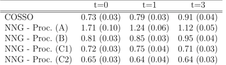
t=0 t=1 t=3 COSSO 0.73 (0.03) 0.79 (0.03) 0.91 (0.04) NNG - Proc. (A) 1.71 (0.10) 1.24 (0.06) 1.12 (0.05) NNG - Proc. (B) 0.81 (0.03) 0.85 (0.03) 0.95 (0.04) NNG - Proc. (C1) 0.72 (0.03) 0.75 (0.04) 0.71 (0.03) NNG - Proc. (C2) 0.65 (0.03) 0.64 (0.04) 0.64 (0.03)
Table 2: Average ISE (estimated by Monte Carlo over 10,000 points) over
100 simulations. V = 5 fold cross-validation is used. Empirical standard
errors are given within parentheses. NNG stands for nonnegative garrote. estimated by Monte Carlo using 10,000 test points generated from the same distribution as the training points.
We begin by examining the predictive ability of each method under three
different designs: t= 0 which corresponds to a uniform independent design,
and t= 1 and 3 which generates covariates with correlations of 0.5 and 0.9,
respectively. Table 2 presents the average ISE over the 100 simulations. If we consider the COSSO results as a benchmark, we see that our proposal can produce similar or better results in its (C) versions. This is particularly true
in the presence of correlation between the x’s (t = 1 and t = 3) where
Pro-cedures (C1) and (C2) have significantly lower ISE. Procedure (B) behaves similarly (or slightly worse) than COSSO. Procedure (A) should be avoided, even though a somewhat strange and unexpected behavior seems to appear: the results get better in the presence of higher correlation.
Table 3 displays the number of times (out of the 100 simulations) that each variable has been selected to appear in the final model. Generally, COSSO tends to include less extra covariates but at the same time misses sig-nificant covariates more often. In contrast, our approaches are more effective
at identifying the signal. In keeping with Shao (1993), who considers good
models as those which contain the true generating model, our approaches should be preferred. Note also that the presence of some extra variables doesn’t seem to impact the predictive ability of our approaches (see Table 2 above).
One has to be careful when reading the results in Table 3 for t = 1 and
t = 3 since the X’s are correlated in these cases, and as a result substitution
can arise. We decide nevertheless to report the results in this manner, given that all of the compared methods are affected in the same way.
We also ran the nonnegative garrote procedures with V = 10 folds. The
Design Technique X1 X2 X3 X4 X5 X6 X7 X8 X9 X10 t=0 COSSO 100 98 100 100 2 1 0 1 0 3 NNG - Proc. (A) 100 100 100 100 23 21 21 15 23 23 NNG - Proc. (B) 100 100 100 100 23 20 27 22 33 15 NNG - Proc. (C1) 100 100 100 100 28 27 35 35 22 30 NNG - Proc. (C2) 100 100 100 100 19 16 19 20 13 19 t=1 COSSO 95 74 100 100 3 12 4 5 10 3 NNG - Proc. (A) 100 100 100 100 13 22 24 28 20 20 NNG - Proc. (B) 99 100 100 100 34 29 32 32 29 28 NNG - Proc. (C1) 100 100 100 100 45 44 37 35 37 32 NNG - Proc. (C2) 99 100 100 100 24 24 22 15 18 18 t=3 COSSO 56 79 94 100 19 23 18 19 20 20 NNG - Proc. (A) 80 100 100 100 33 29 34 35 40 36 NNG - Proc. (B) 87 100 100 100 36 43 34 44 37 46 NNG - Proc. (C1) 90 100 100 100 46 38 39 40 36 41 NNG - Proc. (C2) 79 100 100 100 24 22 23 26 19 22
Table 3: Frequency of appearance of the variables in 100 simulations.
3.2
Simulated example
In this section we construct a model based upon the introductory example on the Boston Housing Data. The aim is to compare the four versions of our technique to common stepwise approaches. We will evaluate the ability of each approach to extract the true underlying model.
We consider the fitted functions of the final model of Section 2 (see Fig-ure 2) to be the “true” functions. The linear predictor is then constructed
with the variables crim, rm, dis, rad,tax, ptratio, and lstat. Finally we
added a normally distributed error term (mean=0, sd=0.1) to simulate the
responses. Variables nox, indus, age, zn and b are considered non
infor-mative. Note that we discard variable chasgiven its binary nature and our
interest in nonparametric fits. In summary, we arrive at a simulated dataset with 7 informative dimensions out of 12.
In Table 4 we summarize the results of 100 simulations by classifying
the final model obtained into one of the following categories: Missing ≥ 2,
Missing 1, True, Extra 1, Extra≥2, or Other. The title of each category
indi-cates the number of missing or extra variables appearing in the final model as compared to the true generating model. Note that the last category, Other, may for example include a final model where a generating variable is miss-ing, but where a variable not used in the construction of the model appears. Procedures (A), (B), (C1) and (C2), as described earlier, are based on our
Missing ≥ 2 Missing 1 True Extra 1 Extra ≥2 Other Proc. (A) 0 0 43 36 21 0 Proc. (B) 2 0 17 30 50 1 Proc. (C1) 0 0 8 26 66 0 Proc. (C2) 0 0 21 34 45 0 Step. (A) 0 0 0 2 35 63 Step. (B) 0 0 1 2 61 36
Table 4: Percentage of models in each category.
nonnegative garrote approach. Step. (A) and (B) refer to stepwise backward variable selection procedures based on an initial choice of the degrees of free-dom as per procedure (A) and (B), respectively. They are both conducted on the basis of an F-test. These latter two approaches are included so as to compare results with what is often done in practice. The four versions con-tained in our nonnegative garrote approach clearly outperform both stepwise approaches in identifying the underlying signal.
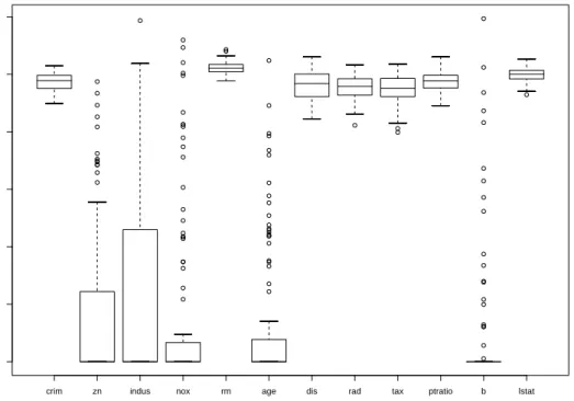
In Figure 3 we present a series of boxplots to show the variability of the
ck values across the 100 simulations. For the informative variables these
boxplots are centered around 1, whereas for the non informative variables
they are shrunken down toward 0. Note that the median of the ck for the
noninformative variables is always zero while the median of the ck for the
informative variables is very close to 1.
4
Discussion
We have proposed a model selection approach based on nonnegative garrote for variable selection in nonparametric regression. We have compared (via simulations) the performance of its four versions to existing methods, e.g. COSSO and stepwise. In terms of predictive ability, versions (C1) and (C2) of our approach perform very well and better than COSSO. Alternative versions (A) and (B) are not as good with respect to predictive ability, but are quite effective in identifying the underlying model, although additional spurious variables are included at times. In contrast, COSSO tends to select smaller models, sometimes missing important variables. Stepwise approaches show a tendency to select very large models, including non significant variables.
Wood and Augustin (2002) suggested an ad-hoc procedure to try to obtain a variable selection procedure from the automatic smoothing parameter selec-tion. Their approach is based essentially on 3 criteria (see their Section 3.3). This involves some manual tuning and is very difficult to implement on a
crim zn indus nox rm age dis rad tax ptratio b lstat 0.0 0.2 0.4 0.6 0.8 1.0 1.2 ck
Figure 3: Boxplot of the values of theckover 100 simulations for each variable
large scale.
Further work includes the extension of this approach to the entire GAM (non normal) class of models and the consideration of resistance-robustness aspects building on work by Cantoni and Ronchetti (2001) and Cantoni, Mills Flemming, and Ronchetti (2005).
5
Acknowledgement
This work has been supported by grant 1214-66989 of the Swiss National Science Foundation. The authors would also like to thank Leo Breiman for providing the code, Sylvain Sardy for helpful discussions and David Conne for providing initial simulation results.
References
Belsley, D. A., Kuh, E., and Welsch, R. E. (1980).Regression Diagnostics:
Identifying Influential Data and Sources of Collinearity. New York: Wiley.
Bock, M. and Bowman, A. W. (1999). Comparing bivariate nonparametric regression models. Technical Report 99-1, Department of Statistics, University of Glasgow, Scotland.
Breiman, L. (1995). Better subset regression using the nonnegative garrote.
Technometrics, 37, 373–384.
Cantoni, E. and Hastie, T. (2002). Degrees of freedom tests for smoothing
splines. Biometrika, 89, 251–263.
Cantoni, E., Mills Flemming, J., and Ronchetti, E. (2005). Variable
se-lection for marginal longitudinal generalized linear models.
Biomet-rics,61, 507–514.
Cantoni, E. and Ronchetti, E. (2001). Resistant selection of the smoothing
parameter for smoothing splines. Statistics and Computing, 11, 141–
146.
Efron, B., Hastie, T., Johnstone, I., and Tibshirani, R. (2004). Least angle
regression. The Annals of Statistics,32, 407–451.
Friedman, J. H., Hastie, T., and Tibshirani, R. (2001). The Elements of
Statistical Learning. Berlin/New York: Springer-Verlag.
Furnival, G. M. and Wilson, Robert W., J. (1974). Regression by leaps
Gu, C. (2002). Smoothing spline ANOVA models. Berlin/New York: Springer-Verlag.
H¨ardle, W. (1990). Applied Nonparametric Regression. Cambridge:
Cam-bridge University Press.
Harrison, D. and Rubinfeld, D. L. (1978). Hedonic prices and the demand
for clean air.Journal of Environmental Economics and Management,5,
81–102.
Hastie, T. J. and Tibshirani, R. J. (1990). Generalized Additive Models.
London: Chapman & Hall.
Lawson, C. and Hanson, R. (1974). Solving Least Squares Problems.
En-glewood Cliffs, NJ: Prentice-Hall.
Lin, Y. and Zhang, H. H. (2003). Component selection and smoothing in smoothing spline analysis of variance models - COSSO. Technical Report 2556, Institute of Statistics, North Carolina State University. Sardy, S. and Tseng, P. (2004). AMlet, RAMlet, GAMlet: Automatic
non-linear fitting of additive models, robust and generalized, with wavelets.
Journal of Computational and Graphical Statistics, 13, 283–309.
Shao, J. (1993). Linear model selection by cross-validation.Journal of the
American Statistical Association, 88, 486–494.
Tibshirani, R. (1996). Regression shrinkage and selection via the Lasso.
Journal of the Royal Statistical Society, Series B, Methodological,58, 267–288.
Wood, S. N. (2000). Modelling and smoothing parameter estimation with
multiple quadratic penalties. Journal of the Royal Statistical Society,
Series B, Methodological, 62,(2), 413–428.
Wood, S. N. and Augustin, N. H. (2002). GAMs with integrated model selection using penalized regression splines and applications to
envi-ronmental modelling. Ecological Modelling, 157, 157–177.
Yuan, M. and Lin, Y. (2006). Model selection and estimation in regression
with grouped variables. Journal of the Royal Statistical Society, Series
Publications récentes du Département d’économétrie
pouvant être obtenues à l’adresse suivante :Université de Genève UNI MAIL
A l'att. de Mme Caroline Schneeberger Département d'économétrie
40, Bd du Pont-d'Arve CH - 1211 Genève 4
ou sur
INTERNET : http//www.unige.ch/ses/metri/cahiers
2006.01 COPT Samuel and Stephane HERITIER, Robust MM-Estimation and Inference in
Mixed Linear Models, Janvier 2006, 27 pages.
2005.04 KRISHNAKUMAR Jaya and David NETO, Testing Unit Root in Threshold
Cointegration, Novembre 2005, 25 pages.
2005.03 VAN BAALEN Brigitte, Tobias MÜLLER, Social Welfare effects of tax-benefit
reform under endogenous participation and unemployment, Février 2005, 42 pages.
2005.02 CZELLAR Véronika, G. Andrew KAROLYI, Elvezio RONCHETTI, Indirect
Robust Estimation of the Short-term Interest Rate Process, Mars 2005, 29 pages.
2005.01 E. CANTONI, C. FIELD, J. MILLS FLEMMING, E. RONCHETTI, Longitudinal
Variable Selection by Cross-Validation in the Case of Many Covariates, Février 2005, 17 pages.
2004.15 KRISHNAKUMAR Jaya, Marc-Jean MARTIN, Nils SOGUEL, Application of
Granger Causality Tests to Revenue and Expenditure of Swiss Cantons, Décembre 2004, 27 pages.
2004.14 KRISHNAKUMAR Jaya, Gabriela FLORES, Sudip Ranjan BASU, Spatial
Distribution of Welfare Across States and Different Socio-Economic Groups in Rural and Urban India, Mai 2004, 66 pages.
2004.13 KRISHNAKUMAR Jaya, Gabriela FLORES, Sudip Ranjan BASU, Demand
2004System Estimations and Welfare Comparisons : Application to Indian Household Data, Mai 2004, 70 pages.
2004.12 KRISHNAKUMAR Jaya, Going beyond functionings to capabilities: an
econometric model to explain and estimate capabilities, Août 2004, 29 pages.
2004.11 MÜLLER Tobias, RAMSES Abul Naga, KOLODZIEJCZYK Christophe, The
Redistributive Impact of Altrnative Income Maintenance Schemes : A Microsimulation Study using Swiss Data, Août 2004, 40 pages.