DigitalCommons@ILR
DigitalCommons@ILR
Labor Dynamics Institute Centers, Institutes, Programs
2012
Differential Privacy Applications to Bayesian and Linear Mixed
Differential Privacy Applications to Bayesian and Linear Mixed
Model Estimation
Model Estimation
John M. Abowd
Cornell University, [email protected] Matthew J. Schneider
Cornell University, [email protected] Lars Vilhuber
Cornell University, [email protected]
Follow this and additional works at: https://digitalcommons.ilr.cornell.edu/ldi Thank you for downloading an article from DigitalCommons@ILR. Thank you for downloading an article from DigitalCommons@ILR. Support this valuable resource today!
Support this valuable resource today!
This Article is brought to you for free and open access by the Centers, Institutes, Programs at
DigitalCommons@ILR. It has been accepted for inclusion in Labor Dynamics Institute by an authorized administrator of DigitalCommons@ILR. For more information, please contact [email protected]. If you have a disability and are having trouble accessing information on this website or need materials in an alternate format, contact [email protected] for assistance.
Differential Privacy Applications to Bayesian and Linear Mixed Model Estimation
Differential Privacy Applications to Bayesian and Linear Mixed Model Estimation
Abstract Abstract
We consider a particular maximum likelihood estimator (MLE) and a computationally-intensive Bayesian method for differentially private estimation of the linear mixed-effects model (LMM) with normal random errors. The LMM is important because it is used in small area estimation and detailed industry
tabulations that present significant challenges for confidentiality protection of the underlying data. The differentially private MLE performs well compared to the regular MLE, and deteriorates as the protection increases for a problem in which the small-area variation is at the county level. More dimensions of random effects are needed to adequately represent the time- dimension of the data, and for these cases the differentially private MLE cannot be computed. The direct Bayesian approach for the same model uses an informative, but reasonably diffuse, prior to compute the posterior predictive distribution for the random effects. The differential privacy of this approach is estimated by direct computation of the relevant odds ratios after deleting influential observations according to various criteria.
Keywords Keywords
Differential Privacy; Statistical Disclosure Limitation; Privacy-preserving Datamining; Linear Mixed Models; Quarterly Workforce Indicators; MLE; REML; EBLUP; Posterior Predictive Distribution; Random Effects. Comments
Comments Suggested Citation Suggested Citation
Abowd, J.M., Schneider, M.J., & Vilhuber, L. (2012). Differential privacy applications to bayesian and linear mixed model estimation. Unpublished manuscript, Labor Dynamics Institute.
Required Publisher's Statement Required Publisher's Statement Copyright held by authors.
Differential Privacy Applications to
Bayesian and Linear Mixed Model Estimation
John M. Abowd,
1Matthew J. Schneider
2and Lars Vilhuber
3April 20, 2012
Abstract
We consider a particular maximum likelihood estimator (MLE) and a computationally-intensive Bayesian method for differentially private estimation of the linear mixed-effects model (LMM) with normal random errors. The LMM is important because it is used in small area estimation and detailed industry tabulations that present significant challenges for confidentiality protection of the underlying data. The differentially private MLE performs well compared to the regular MLE, and deteriorates as the protection increases for a problem in which the small-area variation is at the county level. More dimensions of random effects are needed to adequately represent the time-dimension of the data, and for these cases the differentially private MLE cannot be computed. The direct Bayesian approach for the same model uses an informative, but reasonably diffuse, prior to compute the posterior predictive distribution for the random effects. The differential privacy of this approach is estimated by direct computation of the relevant odds ratios after deleting influential observations according to various criteria.
Index Terms
Differential Privacy; Statistical Disclosure Limitation; Privacy-preserving Datamining; Linear Mixed Models; Quarterly Workforce Indicators; MLE; REML; EBLUP; Posterior Predictive Distribution; Random Effects.
I. INTRODUCTION
In this paper, we investigate two approaches for applying differential privacy to the estimation of Linear Mixed Models (LMMs) and Bayesian Linear Mixed Models (BLMMs). The first approach constructs an efficient, differentially private estimator that converges in distribution to the Maximum Likelihood Estimator (MLE) by using a sub-sample and aggregate algorithm [23]. The second approach produces differentially private linear predictors for regularized Empirical Risk Minimization (ERM) by perturbing an objective function [6]. Our methods harmonize the two approaches using continuous data and make appropriate methodological decisions where theory is missing. For example, the differentially private linear predictors for ERM are classifiers and require a binary dependent variable, but we extend the approach to a continuous but bounded dependent variable.
Statistical disclosure limitation (SDL) and privacy-preserving datamining (PPD) share the common goal of permitting an analyst to draw valid inferences about the properties of confidential data without revealing too much to the analyst about specific entities in the database. One approach to detailed tabulations is to collect data on a sufficiently large number of entities so as to ensure that no published number is based on only a few. As informal as this approach sounds, it lies at the heart of most of the disclosure limitation protocols in use by governmental agencies around the world, and its formalization as identity risk control (in SDL) and k-anonymity (in PPD) provides the basis for many rule-driven publication programs [8]. An alternative approach to protecting the confidentiality of the data provided by the entities that inhabit the levels of a detailed factor is the model-based approach. Model-based procedures combine the data from all of the entities using a formal probability model. The estimate for a particular level of the detailed factor is a function of all of the data [8], [10].
1
: Department of Economics and Labor Dynamics Institute, Cornell University, Ithaca, USA: [email protected]
2
: Department of Statistical Science and Labor Dynamics Institute, Cornell University, Ithaca, USA: [email protected]
The linear mixed-effects model is a canonical form of interest to many because it is the basis for applied work in a wide variety of physical and social sciences. In addition, and perhaps of more interest in our context, it is the statistical workhorse of small area estimation, which is an important part of many statistical agencies’ publication programs [15], [20], [21]. Small area estimation and its counterpart in economic data–detailed industrial tabulation–attempt to estimate regression-adjusted means for classifications that have many levels and are sparsely represented in the underlying confidential data. In linear mixed-effects models, the analyst is often interested in an estimate of the extent to which a particular entity (detailed geographical unit or industry) differs from the average. That deviation is modeled as the realization of a random process, and is estimated conditional on the actual values of a few entities with the particular level of the detailed factor under study.
II. DATA SOURCES
We use the Census Bureau’s Quarterly Workforce Indicators (QWI) as our application of LMM estima-tion to small area and industrial detail data protecestima-tion. (See [1] and [2] for details on the data creaestima-tion.) The QWI data contain employment counts, accessions, separations, job flows, earnings, and explanatory variables of interest–namely, industry, state, county (within state), and date (1990:Q2 to 2010:Q1). The dependent variables of interest here are the job creation rate (J CR), job destruction rate (J DR), accession rate (AR), and separation rate (SR). We model rates instead of levels because the differentially private estimators we consider require a bounded parameter space, and these rates are naturally bounded, which effectively bounds the parameter space for LMMs. Industry, state, and county are categorical variables. Time is an integer-valued variable measured in quarters.
The four rates are defined in the establishment-level micro-data as AR = AE¯, J CR ≡ max 0,E−E¯B , J DR≡max(0,B−E¯E), and SR ≡ S ¯ E, where E¯ ≡ E+B
2 , E is end-of-quarter employment, B is
beginning-of-quarter employment, A is accessions within the quarter, S is separations within quarter. The identity
J CR− J DR = AR−SR holds for all entities and time periods [1]. In this paper we use detailed aggregates published from the micro-data. We are thus treating the detailed publication data as proxies for the micro-data as an experiment in statistical disclosure limitation methods. Only J CR, J DR, and
AR are modeled since SR can be calculated from the identity. Note that J CR and J DR ∈ (0,2) but
AR, SR ∈(0,∞) by assuming B, E, A >0. However, ARand SR are empirically not very large unless an establishment j hires or separates many more employees in a quarter than it has at the beginning and end of the quarter. The dependent variables of interest are specified as rates in the LMM specified in Section III-B and modeled accordingly. Categorical variables take the values of 0 or 1 in the X or Z
design matrices defined below and their respective fixed effects and random effects, β andu,are therefore bounded by the range of the dependent variable.
III. MODELSSPECIFICATION
A. Linear Mixed Model
1) Background: One purpose of the classical Linear Model (LM) is to estimate the numerical relations between dependent and independent variables. The two requirements of the LM are: first, that the average value of the dependent variable,J CR, is a linear combination of known data (e.g.,industry and time) and other unknown constants (β, fixed effects) and second, that the dependent variable is normally distributed with a mean at the value of the linear combination. When some of the parameters of the LM are treated as realizations of random variables instead of unknown constants, the model is called a Linear Mixed Model (LMM). In other words, when the mean of J CR is a linear combination of constant terms and random terms which are not constants, the model is a LMM [16]. In our case, some of the random variables are county random effects and we assume that they come from a random sample of counties from the entire population of counties. The LMM allows for J CR to depend on the county and we expect each county’s random effect to be 0 with uncertainty according to a normal distribution. However, for this application, we are not only interested in estimating the variance of county effects (i.e., how much J CR varies due to particular counties alone), but also in the particular level of the realized county random effect, uˆc.
2) Linear Mixed Model Specification: Our statistical model is specified as follows:
y=Xβ+Zu+ξ (1)
wherey(N×1)consists of elementsyjsct,the value of one of the dependent variables(J CR, J DR, AR).
The subscriptj is industry(20), sis state (48), cis unique county within state (3,111), t is time (quarters from 1990:2 to 2010:1), and N is the total number of observations. X is the (N ×21) design matrix for the fixed effects (industry and the time trend). Z is the (N ×3,159) design matrix for the random effects of state and county (within state). Finally, ξ is the (N ×1) observational random effect across all observations and is assumed independent and identically distributed. βˆ is the vector of maximum likelihood estimates (MLEs) and uˆ is the vector of empirical best linear unbiased predictors (EBLUPs). Random effects are assumed independent with a constant variance for each state, county, and observation.
The mixed-effects likelihood function is constructed by assuming
ξ∼N(0, σ2ξIN) = N(0, R), R=σξ2IN us ∼N(0, σs2I48), uc∼N(0, σc2I3111) u= (uTs, uTc)T ∼N(0, G) G= σs2I48 0 0 σ2cI3111
These assumptions imply
E[y|X, Z] =Xβ, y ∼N(Xβ, ZGZT +R) = N(Xβ, V) and given random effects due to state and county:
E[y|X, Z, u] =Xβ+Zu,(y|u)∼N(Xβ+Zu, σ2ξIN)
which implies equation (1).
Henderson [14] shows that maximizing joint density of y and u, yields the MLEs βˆ and EBLUPs uˆ that solve:
XTR−1Xβˆ+XTR−1Zuˆ=XTR−1y ZTR−1Xβˆ+ZTR−1Zuˆ+G−1uˆ=ZTR−1y
Additionally, we are interested in estimating the three variances, σξ2, σs2, and σ2c for statistical inference and the generation of the EBLUPs.
3) Maximum Likelihood and Restricted Maximum Likelihood Estimates: To calculate all estimates of interest, we use the lmer() function from the R package lme4, which maximizes the restricted log-likelihood, called REML [5] and takes advantage of sparse matrix computations [3]. Table I shows a summary of the REML estimates produced for our model. Initial global estimates are calculated from Table I independently for each of the three modeled rates (J CR, J DR, and AR) using the original data (about 2.4 million rows). These estimates (βˆglobal,uˆglobal,ˆσglobal) act as a benchmark for the differentially
private methods in this paper that use sub-sampling and Laplace noise (βˆDP,uˆDP,σˆDP). Section IV
provides more details.
Estimates of the LMM parameters are produced by minimizing the negative log-likelihood (MLE) or restricted log-likelihood (REML). Although there is no closed form solution for the MLE or REML of the complete parameter vector β, G/σ2ξ, σξ2 [4], [7], Bates and Debroy [4] show that intermediate REML calculations for the parameters in G/σ2
ξ can be expressed using a profiled log-restricted likelihood that
only depends on a G/σ2
ξ and not β, σξ2
.
Estimate Dimension Description ˆ β1,...,β20ˆ 20 Industry (n) MLEs ˆ β21 1 Quarter (t) MLE ˆ
u1,...,u48ˆ 48 State (s) BLUPs
ˆ
u49,...,u49+3110ˆ 3111 County (c) BLUPs
ˆ σ2ξ 1 Residual Variance ˆ σ2s 1 State (s) Variance ˆ σ2 c 1 County (c) Variance TABLE I ESTIMATEDESCRIPTIONS
B. Bayesian Linear Mixed Model
1) Background: Bayesian estimation of the LMM permits us to incorporate both a priori knowledge of the parameters, β, σ2
uc, σ2ξ, and information from the data, (y, X, Z), into the fitting of the BLMM to
generate samples from the posterior distribution of β, σuc2 , σ2ξ, andu. We set the prior distribution ofβ, σuc2 ,
and σ2ξ to their feasible ranges and use the samples from the posterior distributions to directly analyze the privacy properties of the fixed effects, variance components, and estimated random effects. We compare the posterior draws of the sensitive county random effects, u, from a BLMM fit with all observations (benchmark fit) to BLMMs fit by deleting one influential observation at a time. We then calculate the maximal differential privacy risk over all the single-row deletion experiments. This procedure produces an empirical DP.
2) Bayesian Linear Mixed Model Specification: Our BLMM model is specified as follows:
y = Xβ+Zu+ξ
R = σξ2I, G=σuc2 I
ξ∼N(0, σ2ξIN) = N(0, R), R=σξ2IN
u∼N(0, σ2ucI3111) = N(0, G)
σξ2 ∼IW(V, v), σ2uc∼IW(V, v), β ∼M V N(µ,Σ)
wherey(N ×1)consists of elements yjct,the value of one of the dependent variables(J CR, J DR, AR).
The subscript j is industry (20), c is unique county (3,111), t is lagged quarterly rates(4×1) , and N
is the total number of observations. X is the (N×24) design matrix for the fixed effects (industry and lagged rates). Z is the (N ×3,111) design matrix for the random effects county.
For the BLMM we consider only unique county random effects and discard state random effects; hence the estimated county effects are actually the sum of the state and county(within state) effects. The prior distributions of the variance components are multivariate Inverse-Wishart distributions (V, υ) that reduce to Inverse-Gamma distributions when V is a scalar, as above. Some advantages of the Inverse-Wishart and Inverse-Gamma distributions are that their random variables are always real-valued positive definite matrices and positive reals, respectively, and they are the conjugate prior distributions for the multivariate normal and univariate normal distributions, respectively [11]. The prior distribution of the fixed effects is a multivariate normal distribution (µ,Σ)that allows for more complex covariance structures. Our model is similar to the LMM in Section IV except for the additional covariates that model the time structure more accurately and the use of Markov Chain Monte Carlo (MCMC) sampling instead of REML estimation. The outputs of MCMC are draws from the posterior distribution of the parameters and the random effects while the outputs of REML are point estimates. MCMC from BLMMs gives us greater flexibility in
analyzing the tails of the posterior distribution of the parameters and random effects for differential privacy applications.
3) Posterior Distribution: Ten thousand samples of the parameters, β, σuc2 , σ2ξ, and u, are drawn from their posterior distributions after burn-in. Then, posterior samples from the distribution of ucare generated
from Pr(uc|y, X, Z, β, σξ2, σuc2 ) for every county c. See Section V for further details.
IV. DIFFERENTIALLY PRIVATEESTIMATION VIA SUB-SAMPLING
We use LMMs and Smith’s [23] differential privacy via random sub-sampling method to compute a differentially private MLE from our data by means of partitioning the complete sample into thousands of disjoint LMMs that share the same parameter vector and random effects, although only a subset of the random effects appear in any given sub-sample. The QWI data are used to form the matrices X and Z, and the vector y, which we use in this algorithm. Although we are using public data, the exercise nicely simulates protecting the confidential entity data since we are trying to summarize the characteristics of a large number of states, counties, industries, and time periods. We have not yet focused on the time effects because we are concerned with showing the effects of SDL or PPD on the small area estimates (counties within state). The time effects are given further consideration in Section V with the BLMMs. We apply Smith’s method of differential privacy via sub-sampling [17], [23] directly to the full data matrix from the QWI.
A. Sub-sampling
Divide the input (y, X, Z)into k disjoint blocks,i.e.construct sub-samples by rows,B1, ..., B(i), ..., Bk
of nk = bNkc points each where B(i) denotes the ith disjoint subset and N is the total number of
observations. The complete data set for each of the three models is denoted by(y, X, Z) =S
(y1, X1, Z1), ..., (y(i), X(i), Z(i)), ..., (yn, Xn, Zn). Using lmer(), calculate k sets of estimates from Table I using the
data for each block only.
B. Bias-corrected βˆ(i) and uˆ(i)
McCulloch and Searle [16] note that the solutions to Henderson’s equations areβˆ= (XTV−1X)−1XTV−1y
andBLU P =GZTV−1(y−Xβˆ),whereV =ZGZT+R. Both of these equations are functions of at least
one variance component of the model within R or G, which are not known, and must be estimated. Since the variance components are estimated, our estimate of uisEBLU P(u) = ˆu= ˆGZTVˆ−1(y−Xβˆ). Prasad
and Rao [21] state that the resulting two-stage estimator is unbiased if the expectation of the estimator is finite, the elements of the estimated variance components are even functions of yand translation-invariant, and the distributions of u and ξ are both symmetric. Our empirical results suggest that our EBLUPs are more biased as we increase the number of sub-samples k. Additionally, the estimated variance components become larger as k increased. We implemented a bias-corrected version βˆ(i) anduˆ(i) for the differentially
private estimate generation routine.
The bias-corrected estimates are produced as follows. Calculate βˆglobal, uˆglobal, σˆ2global
ξ , σˆ
2global
s , and
ˆ
σ2global
uc for all of the data when k = 1. For each block (i), subtract βˆglobal and uˆglobal from βˆ(i) and ˆ
u(i), respectively. Call these βˆ(bci) and uˆbc(i). For each block (i), subtract σˆ 2global ξ , σˆ 2global s , and ˆσ 2global uc from ˆ
σξ2(i), σˆ2s(i), and σˆ2uc(i), respectively. Call these σˆ2ξbc(i), σˆ2sbc(i), and σˆuc2bc(i). For each block (i), regress (βˆ(bci), ˆ
ubc(i))1 on ˆσ2bc
ξ (i), σˆs2bc(i), and σˆuc2bc(i) and obtain estimates γˆξ(i), γˆs(i), and γˆuc(i) for each regression. For
each block (i), obtain fitted values of βˆbc
(i) and uˆ bc (i). Call them βˆ bc∗ (i), uˆ bc∗
(i). Obtain the bias-corrected βˆ(i)’s
and uˆ(i)’s to use in the differentially private estimate generation routine by setting βˆ(i)= ˆβ(i)−βˆ(bci)∗ and ˆ
u(i)= ˆu(i)−uˆbc(i)∗.
1
C. Averaging Sub-samples as the Aggregation Function
Average the estimates over k blocks:
ˆ β∗∗= k P i=1 ˆ β(i) k ,uˆ ∗∗ = k P i=1 ˆ u(i) k , ˆ σ2s∗∗= k P i=1 ˆ σs2(i) k ,σˆ 2∗∗ c = k P i=1 ˆ σ2c(i) k , and ˆ σξ2∗∗= k P i=1 ˆ σξ2(i) k
Next, draw Rβ, Ruand Rσfrom independent Laplace distributions, as a function of the differential privacy parameter , where the Laplace scale parameters b = (b1, b2, b3) are
Λβ k, Λu k, and Λσ k, respectively, and ˆ σ = (pσˆ2∗∗ s , p ˆ σ2∗∗ c , q ˆ σ2∗∗
ξ ). The valuesΛβ,Λu, andΛσ are the global sensitivities [23] or the maximum
ranges of the parameters β, µ, and σ, respectively, as shown in Table II. Output βˆDP = R
β + ˆβ ∗∗ , ˆ uDP =R u + ˆu ∗∗ and σˆDP ξ =Rσ + ˆσ ∗∗
as the differentially private estimates with protection .
In the process of sub-sampling disjoint subsets from over 2.4 million observations or rows in the matrices
X and Z, individual subsets could contain between 271 (for = 1) and 500 (for = 4.6) observations where the sample size of the individual subset is nk=
N k =j N Λ 2/5k
as derived in Section IV-D. For large values of k, it is very likely that many of the sub-samples do not have entries for some industries, many states, or thousands of counties in the X(i)or Z(i) matrices due to chance or the limited number of
rows (nk). Consequently, many of the their respective parameters cannot not be estimated. In such cases,
we treat these non-estimable βˆ(i) and uˆ(i) as missing, and do not use them in our averaged estimates.
In cases with even smaller individual subsets (e.g., when k = 16,000, nk = 151), it is possible that the
mixed model is not estimable. Therefore, we must keep k at a reasonable level and in Section V, we use
k = 8,945 (= 1) through k = 4,858 (= 4.6).
County effects were considered a random effect since there were 3,111 unique counties corresponding to different states and each sub-sample contained a random subset of counties from the universe within that state. State effects were also considered random, but always had less than one-fourth of the states missing observations in the Z(i). For k= 8,945 in all sub-samples, industry had at most 1 or 2 industries
missing from X, state had between 0 and 11 states missing (an average of 4 missing) fromZ, and county had between 2,863 and 2,892 counties missing from Z. In cases where there were many unique counties missing, the estimated variance of the random effect due to unique county, σˆ2
c, was often zero due to the
lack of repeated observations per unique county. Low prevalence categories in industries, such as industry 92 (Public Administration), had many fewer observations than others and, consequently, had higher ranges of estimated coefficients from sub-sample to sub-sample.
The Laplace scale parameters, b, are dependent onΛ, , andk. By fixingk andΛ, the resulting Laplace scale parameters become a function of alone, which we tried to vary from 0.1 to 4.6, but values less than unity for were not estimable.
The Λβ, Λu, and Λσ are maximum ranges in the corresponding parameters of β, u, and σ as shown in
Table II. For J CRand J DR, all three components ofσˆ are bounded since standard deviations should be a maximum of 0.5 for rates ∈(0,2). So, we set Λσto 0.5. βˆanduˆ depend on the scale of the data, which
in our case contains only 0 and 1 except for the time trend variable. In such binary cases and disregarding any interactions, we set Λβ and Λu to be 2. In simulations, the quarter estimate, βˆ21, always had a very
low range across sub-samples (less than .004), so Λβ21was set to .01 because 2 would be too large for
For AR, the bounds need to be larger to account for the empirical range of AR ∈ (0,385), which is much too large for meaningful statistical inference when this range is used to set the Laplace scale parameter for the differentially private estimates. We calculate empirical ranges of the parameter estimates over different values of k for all rates in Table II. When looking at the 0% to 99.9% quantile of AR, the rates are ∈ (0,2.57). Consequently, Λσwas set to 0.75, Λβ and Λuwere set to 3, and Λ21was set to 0.01
(from empirical simulation). Table II shows the maximum ranges of estimates for J CR and AR over
k = 8,945 sub-samples, which always had larger maximum ranges than smaller k in our simulations. Estimate JCR Max Range JCRΛ AR Max Range
ˆ β1,...,β20ˆ 2.49 2.0 49.6 ˆ β21 0.003 0.01 0.15 ˆ u1,...,ˆu48 1.67 2.0 9.6 ˆ u49,...,u3161ˆ 2.04 2.0 374.5 ˆ σξ2 0.20 0.5 5.5 ˆ σs2 0.26 0.5 1.6 ˆ σc2 0.19 0.5 24.1 TABLE II
MAXIMUMEMPIRICALRANGES
D. Number of Sub-samples
Smith [23] shows that the maximum number of sub-samples to be considered is k = n2/3 to get a
sufficiently small bias, and the optimal number of sub-samples is k∗ = n3/52/5Λ2/5 to get an asymptotic
relative error that tends to 1. Setting Λβ and Λu equal to the maximum of all estimate ranges for the
J CR and J DR models implies an optimal k∗of 8941 . As ranges from 0.1 to 4.6, the optimal k∗ranges from about 22,470 to 4,858. Results are presented using ∈ (1,2,3,4,4.6). A value of k∗ > 9,000 is not feasible within the REML computation because the low sample size (nk = 151) does not permit any
estimation at all.
E. Differentially Private Fitted Values
The fitted values of our mixed model are linear combinations of the rows of X and Z and the differentially private estimates with protection . X and Z are sparse matrices because the columns are categorical variables and any given row is identified by an industry, unique county, and quarter. Any fitted value is the sum of three differentially private estimates with protection and a quarter, t, times the differentially private trend estimate, βDP
21 , with protection . Ignoring the differentially private trend
estimate, βDP
21 , and assuming each row can only change by industry and unique county, we provide a
proof for differentially private fitted values that builds on Smith’s proof [23].2
Lemma 1: For any choice of the number of sub-samplesk, a fitted value for any row isC-differentially private where C is 2, the assumed number of non-zero entries inX andZ for an added or deleted row r.
Proof: Given fixed matrices of X and Z, consider adding or deleting a row r to obtain neighbor matrices X0 and Z0 that differ from X and Z by only by one observation or row. At most, only one of the sub-samples B(i) = (y(i), X(i), Z(i))can include or exclude row r. The maximum that the components
of βˆ(i) and uˆ(i) can change with or without row r is by their global sensitivities, Λβ and Λu. Therefore,
the most βˆ∗∗ = k P i=1 ˆ β(i) k and uˆ ∗∗ = k P i=1 ˆ u(i)
k can change are
Λβ
k and
Λu
k , respectively. By Smith [23], this
results in the Laplace random variables βˆDP =R
β+ ˆβ
∗∗
and uˆDP =R
u+ ˆu
∗∗
each being-differentially private where the Laplace noises were defined in Section IV-C. Define an arbitrary fitted value of the
2tΛ
β21≤101(.01) = 1.01 So,tΛβ21 <Λβand by using the Laplace scale parameter,R
β, forβ21,β DP
vector yˆDPC = XβˆDP+ZuˆDP as yˆDPc
a . yˆDPa c is a function of two -differentially private estimators
without using additional confidential data (X and Z are not confidential) and therefore, 2-differentially private.
Note that the proof can be generalized to different allocations of privacy, such as two estimators that are 0.1-differentially private and 0.9-differentially private by changing the Laplace scale parameters. The result is that a fitted value for any row would be (0.1 + 0.9)-differentially private or -differentially private. We generalize the proof to three differentially private estimators for the industry effect, trend effect, and unique county EBLUP. All figures use a total of -differential privacy with varying levels of the privacy budget for β and u, and an allocation of 2% of for β21. Additionally, we did 30 random
simulations of differentially private fitted values and averaged the correlation results in Figures 2,3,4,5,6, and 7.
V. DIFFERENTIALLYPRIVATE ESTIMATION VIAEXPECTEDRISKMINIMIZATION
We use BLMMs for Chaudhuri, Monteleoni, and Sarwate’s [6] approach of differential privacy and relate the posterior distribution of the BLMM to ERM. Their approach shows that -differential privacy can be obtained by perturbing an objective function, Jpriv, to obtain an efficient, differentially private
approximation for the predictors, fpriv, of regularized ERM.
fpriv = arg minJpriv(f,D) +
1 2∆kfk 2 = arg min[1 n n X i=1 `(f(xi),yi) + ΛN(f) + 1 nb Tf] +1 2∆kfk 2
fpriv, or more commonly known as regression coefficients (β) in Generalized Linear Models such as the
logistic regression, is obtained by minimizing a loss function and a regularizer [6]. One major difference between their approach and ours is that the objective perturbation algorithm relies on classifiers for binary dependent data and our applications has continuous dependent variables. Thus, the original Cahudhuri et al. algorithm contains natural parameter bounds and frees their privacy parameter from dependence on the sensitivity of the classification algorithm. In our application, we use bounded continuous rates and define an informative prior distribution that bounds the parameters in the posterior distribution from which we calculate the empirical level of .
We note that regularized risk minimization is equivalent to maximum a posteriori estimation and arg min[1
n
n
X
i=1
`(f(xi),yi) + ΛN(f)] = arg min[Empirical Risk+Regularizer]
= arg min[−logL()−logp(f)] = arg max [ log (L()×p(f))] = arg max [L()×p(f)] = arg max [posterior]
We proceed in the Bayesian fashion by setting priors on our fixed effects and variance components. Then, we fit the complete-data model. Next we remove influential observations one at a time in order to estimate the effective -differential privacy of the complete-data procedure. We analyze effects on the posterior distribution of the complete set of uc, the county random effects because these are much more
sensitive to a breach in privacy than the fixed effects or variance components.
A. Prior Specification
We use the multivariate Inverse-Wishart distributions(V, υ)and multivariate normal distribution(µ,Σ). To test the feasibility of differential privacy for the BLMM we consider the simplest case of such distributions, although we are not limited to such. We use the univariate Inverse-Wishart, which becomes an Inverse-Gamma(υ
2,
υV
2 )distribution with mean
υV
ν−2 and variance
v2V2
(υ−2)2(υ 2−2)
We also set the prior of our fixed effects at µ= 0 and Σ∝I causing the multivariate normal distribution to produce independently and identically distributed univariate normal distributions with mean zero and constant variance a priori. In order for our priors to depend on only one parameter, υ, the degrees of freedom, we set V equal to a constant. Our benchmark and confidential prior distribution, p0, is diffuse
with the bounds being set as close as possible to the feasible ranges of the parameters β ∈ (−2,2) and
σ2
uc, σξ2 ∈ (0, .25). When setting V = .104 and υ = 12, the prior mean and standard deviation of σuc2
and σ2
ξ are .125 and .0625, which we define as the benchmark prior, p0, that spans the feasible range
of our variance components. We also set Σ = 162 v2V2
(υ−2)2(υ 2−2)
I to ensure the standard deviations of our benchmark univariate normal priors are 1, span the feasible range of β, and scale with the priors of σ2
uc
and σ2
ξ. This gives the following BLMM:
Y = Xβ+Zu+ξ R = σξ2I, G=σ2ucI p= (σξ2 ∼IG(υ 2, vV 2 ), σ 2 uc∼IG( υ 2, vV 2 ), β ∼M V N(0,16 2 v2V2 (υ−2)2(υ 2 −2) I)).
B. Bayesian Computation and -Differential Privacy
We use the R package MCMCglmmto fit the BLMM through MCMC simulation.MCMCglmmuses C++, samples all location parameters in a single block, uses CSparse C libraries, and is 40 times faster than Winbugs [12]. Even with these advantages, for our data it takes about 10 hours to run 20,000 MCMC iterations with a 10,000 iteration burn-in and thinning interval of 5. To incorporate the intuitive notion of differential privacy for the sensitive county random effects, we remove one observation from our data set and rerun the BLMM to generate the new posterior distribution of u. We use influence diagnostics geared for the LMM to choose those observations that require closer examination for the BLMM.
1) Influential Observations: We delete observations i that are most influential on the EBLUPs of our LMM under REML estimation and later fit a separate BLMM for each of those observations deletions. Traditional influence diagnostics for the LM are not completely transferable to the LMM because βˆand uˆ are functions of the estimated variance components,σ2
ξ andσ2uc. For example, the residuals of the LMM do
not have to sum to zero and can sometimes produce negative values of leverage located on the diagonals of the “hat matrix,” H =X(X0Vˆ−1X)−1X0Vˆ−1 [22]. Since the LMM should be refit when deleting each observation i to know exactly how estimates change, we incorporate several notions from the influence diagnostic literature to select observations that are influential on the entire model or specific EBLUPs.
Define the marginal residuals given the fixed effects as yi −x0iβˆ and the conditional residuals given
the EBLUPs as ri = yi −x0iβˆ−zi0uˆ. Assuming the variability of βˆ is negligible given the sample size
of our data, we calculate the Pearson residuals given the conditional variances as rpi = √ ri
V ar(Yi|u)
= ri
σ2 ξ
which in our LMM is simply proportional tori due to the simple covariance structure and conditioning on
the EBLUPs. Schonberger suggests calculating conditional residuals and conditional Pearson residuals for influence diagnostics in the LMM [22]. Nobre and Singer [18] suggest looking at a standardized version of the conditional residuals by dividing rpi by a function of the joint leverage of the fixed and random effects for detecting the presence of outlying observations. They also reference Pinheiro and Bates [19] who suggest looking at extreme values of uˆ for detecting the presence of outlying EBLUPs.
We selected 32 influential observations to examine. First, we selected 14 observations with the most extreme positive or negativerpi values. Second, since our design matrix,Z, is unbalanced with five counties containing fewer than 15 observations, we selected 10 observations with the minimum and maximum rpi
from each of those counties. Finally, we selected eight observations with the minimum and maximum rpi
2) Differential Privacy of the Realizations of County Random Effects: We create a methodology for calculating-differential privacy for continuous data using the posterior distribution ofufrom our BLMMs. First, we generate 10,000 samples from the posterior distribution of β, u, σuc2 ,and σ2ξ from our benchmark model with prior p0 and all observations (after discarding the 10,000 burn-in samples). Then, we remove
influential observationi, refit our model with the same priorp0, and also generate 10,000 posterior samples
(again, after discarding the 10,000 burn-in samples). We estimate the changes for the tails of the posterior distribution of u between the benchmark model and a model missing an influential observation.
For our models let
D ≡ (y, X, Z), entire data set
and D˜i ≡ (y˜i, X˜i, Z˜i), the data set without observation i.
Define the posterior odds as P0(uc|D˜i)
P0(uc|D) and the prior odds as
P0(uc)
P0(uc) for all county-effect posterior
distribu-tions of the random effect uc.3 Bounding the maximum and minimum of the posterior odds ratio
M1 ≡max i,c P0(uc|D˜i) P0(uc|D) Pm(uc) P0(uc) = max i,c P0(D˜i|uc) P0(D|uc) and M2 ≡min i,c P0(uc|D˜i) P0(uc|D) Pm(uc) P0(uc) = min i,c P0(D˜i|uc) P0(D|uc)
is equivalent to the requirement for −differential privacy by setting = max (|lnM1|,|lnM2|)[9]. Since
the prior odds were defined unconditional on the deleted observation i, we assume that the prior odds ratio is 1, and we only need to focus on the posterior odds to determine .
One method of calculating the posterior odds is to fit a kernel density estimator of the posterior samples ofu, and then evaluate these ratios over narrow bin widths. We found this method to be overly sensitive to posterior samples in the tails of the posterior distribution. Instead, we approximate max (|lnM1|,|lnM2|)
by comparing the number of tail occurrences between the benchmark model and models missing an influential observation using a discretized posterior with 20 bins. Given 10,000 posterior samples of each
uc|D from the benchmark model, we create 20 bins of 500 samples corresponding to the five percent
quantiles of the benchmark posterior samples. Then, for each model with deleted observation i, we count the number of posterior samples, ni,c,b of uc|D˜i within each of the benchmark bins. Over all models
without i, county random effects (c = 1,2, ...,3111), and bins (b = 1,2, ...,20) compute ni,c,b
500 and set = max (|lnM1|,|lnM2|) where M1 = max
i,c,b ni,c,b 500 and M2 = min i,c,b ni,c,b 500 .
3) Convergence: We monitored convergence for the benchmark model by performing two iterative sim-ulations (with dispersed initial conditions) and evaluating the Gelman and Rubin convergence diagnostic. Each simulation was run for 10,000 iterations after a burn-in of 10,000 samples. The Gelman and Rubin convergence diagnostic measures the between-sequence variance,B, and the within-sequence variance,W, for two or more iterative sequences. It outputs a potential scale reduction factor,
qn−1
n W+ 1 nB
W , that declines
to 1 as the number of posterior samples, n, goes to infinity [11]. Gelman, Carlin, Stern, and Rubin note that for most examples, scale reduction factors below 1.1 are acceptable. The upper confidence limits of the potential scale reduction factors for our 3,111 county-wide random effects, two variance components, and 24 fixed effects were always between 0.99990 and 1.0047 except for county random effect u1460 at
1.2853 which only had 58 observations. We examined the trace plots for county random effect 1460 in Figure 1 below and found no issues with convergence.
3
Fig. 1. Trace Plots of County 1460
VI. RESULTS
A. Linear Mixed Models
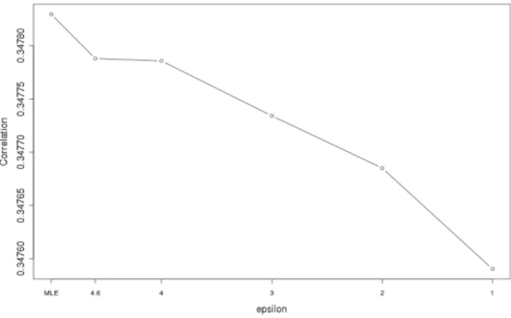
We produced R −U (Risk-Utility) curves or R−U confidentiality maps that examine the trade-off between (disclosure risk) and correlations (data utility) by changing parameter values in our procedure. Duncan [8] states that “in its most basic form, an R−U confidentiality map is the set of paired values (R, U) of disclosure risk and data utility that correspond to various strategies for data release.” In our models, changes to generate the R−U curve and lower values of correspond to lower levels of risk and higher levels of privacy. As decreases, the privacy of our released data increases as defined by
-differential privacy. Low disclosure risk has good differential privacy, which says that “any possible outcome of an analysis should be “almost” equally likely, independent of whether any individuals opts into or opts out of the data set” [9]. In addition, since the Laplace scale parameter is kΛ, the random noise added to release -differentially private data increases as decreases (k increases at a slower rate than decreases). This means that the released data or estimates are more noisy for lower values of . Consequently, data utility should be lower for released data with more noise added. We examined the exact trade-off between disclosure risk, , and data utility, correlation (ˆyDP,y).
1) R−U Curve for Linear Mixed Models: For all values of , calculate the predicted rates:
J CRDP = ˆyDP =XβˆDP.51+ZuˆDP.49
For k = 1 or all of the data, calculate the predicted rates:
J CRglobal = ˆyglobal=Xβˆglobal+Zuˆglobal
Calculate the correlations between y and yˆglobal, yˆDP. Finally, plot the correlations as a function of .
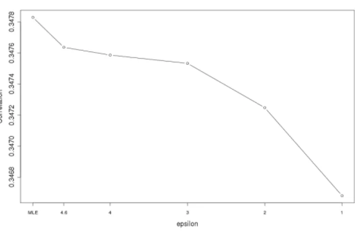
2) R−U Curve for Linear Models: For all values of , calculate the predicted rates:
J CRDP = ˆyDP =XβˆDP
For k = 1 or all of the data, calculate the predicted rates:
Calculate the correlations between y and yˆglobal, yˆDP. Finally, plot the correlations as a function of .
The LM only estimated industry means and did not include a time trend.
Figures 2 and 3 show the R-U Curves for the LMMs and LMs, respectively. Correlations decreased as
decreased, and all correlations of yˆDP with y were lower than the global “best fit” correlation when
k = 1 (which would correspond to non-differentially private >25). Since all correlations including the one between y and yˆglobal were less than 0.40, the model did not fit the data well. This illustrates the
principle limitation of the differentially private estimator – more random effects were required to get a good fit, detailed industry and time effects in particular, but such models were only feasible when >25,
which is no protection at all. But for models with approximately 3,000 effects, degradation in correlation over decreased values of was only slightly noticeable. Non-monotonicity was observed when most of the noise was added to β versus u since there were only 21 random Laplace draws.
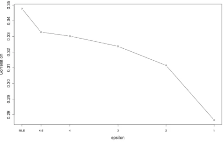
3) R-U Curve for Linear Mixed Models with Allocated Privacy: Additionally, we considered having proportionally different levels of privacy for β anduwithin the total privacy budget of. Since there were many more estimates of u (3,161) as compared to industry β (20), it may be reasonable to protect the estimates of u with more privacy (lower ). Figures 4 and 5 show u having 10% and 88% of the plotted value of , respectively, while β accounts for the remainder. For example, in Figure 4, the five budgets of used for u were 0.46,0.4,0.3,0.2, and 0.1 while the budgets used for β were 4.05,3.52,2.64,1.76,
and 0.88. Figures 6 and 7 show u having 1% and 97% of the plotted privacy value of , respectively. Noticeable degradation is seen in Figure 6 when u is highly protected. For all figures except Figure 3, the privacy budget of the time trend was kept at 2%.
4) An Improved LMM and Influential Observations: We also examined the effects of deleting all of a county’s U observations on the estimates of variance components and fixed effects with a LMM that included four parameters for lagged quarterly rates. The base fit of the model improved significantly to a correlation of 49.67% as compared to just under 35% for the LMM including only a simple time trend. The goal was also to bound the possible leave-1-out changes of our REML estimates, β,ˆ σˆξ2,and ˆ
σuc2 for closer inspection for both the LMM and BLMM. We performed over three thousand leave-U-out simulations for each county. For each simulation, the process is as follows:
• Define D˜U ≡(y˜U, X˜U, Z˜U), differing by one county-industry combination (U-out); • Fit REML estimates and analyze changes in β,ˆ σˆξ2,and σˆ2uc.
Results for the leave U-out fixed effects indicate that all industry estimates are within 0.0002 of each other except for public administration, which has a range of 0.003. The covariates for the lagged quarterly rates were all within 0.001 of each other. The 0.1 and 99.9 percent quantiles for the variance components are described in Table III.
Variance Component MLE 0.1% quantile 99.9% quantile
ˆ
σξ2 0.01045409 0.01043703 0.01046005
ˆ
σ2uc 0.00016302 0.00015722 0.00016330
TABLE III
VARIANCEESTIMATERANGES FROMLEAVING OUTONECOUNTY
Results from the analysis of deleting influential observations from Section V indicate that all updated estimates of fixed effects and variance components are well within the bounds of the leave U-out changes. The county EBLUPs that were most affected by the removal of influential observations were always the particular counties that these observations were in. The maximum change for the EBLUPs was 0.007828 (observation from county 3047) and the industry fixed effects was 0.00008281 (observation from county 661). Both of these observations came from observations with large uˆ’s and large absolute values of
rip. If we were to match these maximum changes correspond to four times the standard deviation of a Laplace random variable, they produce Laplace scale parameters of 0.0015 and 0.000016, respectively. To put things in perspective, the laplace scale parameter for the estimated fixed effects and EBLUPs in the
sub-sample and aggregate approach when was unity was approximately 0.0002 and was was 3 was approximately 0.00012. With no sub-sampling and the removal of an influential observation, the laplace noise would only protect the fixed effects. Results for the BLMM focus on the county random effects.
B. Bayesian Linear Mixed Models
We analyzed the implications of the removal of influential observations on the -differential privacy of our county random effects according to Section V-B.2. Predictably, in those models deleting observations from small counties (3047 and 661) produced the largest proportional bin changes across all models. Each model had 62,220 bins corresponding to 20 bins for each of the 3,111 county random effects. The model deleting an observation from county 3047 had as few as 21 posterior samples in its smallest bin (3,217 in its largest) and the model deleting an observation from county 661 had 3,458 posterior samples in its largest bin (26 in its smallest). Both of these unusual counts occurred in the county effect from which the influential observation was deleted. Comparing these results to the benchmark model with 500 observations in each bin and using the methodology developed in Section V-B.2, this corresponds to an overall of 3.2.
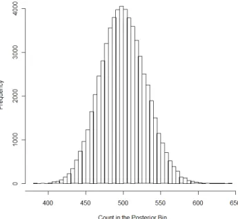
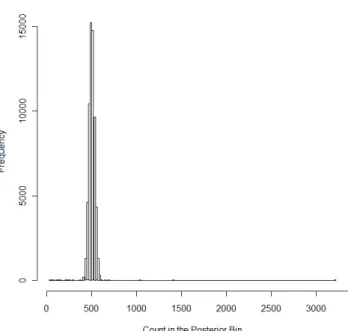
We compared these results to random noise which is represented by the replicated benchmark model that was fit to monitor convergence in Section V-B.3. The bin boundaries were fixed at the five percent quantiles from the complete-data estimation. Hence, the expected count in each bin is 500. The replicated model using the complete data had its smallest bin containing 382 posterior samples and its largest bin containing 641 posterior samples. This corresponds to an overall of 0.27, which is illustrated in the histogram of the bin counts shown in Figure 8 where the mode is 500, the distribution is symmetrical, and the minimum and maximum on the horizontal axis define the inputs to computing . Since no rows have been excluded from this experiment, the interpretation ofis the deviation in the empirical differential privacy that results from the imprecision of using 10,000 posterior samples.
The 32 models with deleted influential observations always had maximum and minimum bin counts between the extremes of the replicated benchmark model and the models with deleted observations from county 3047 or county 661. That is, the extreme values used to estimate empirically came from the values computed when influential observations were deleted from these one of these two counties. A histogram of the bin counts for the model deleting an influential observation from county 3047, which defined the overall of 3.2, is shown in Figure 9.
Fig. 2. R-U Curve for JCR Linear Mixed Model with 49%budget forβand 49% foru
VII. DISCUSSION
Results are presented forJ CRonly; however,J DRandARgive similar results. The main difference in the structure ofARisΛ, which is slightly larger. Thus, the Laplace scale parameter is also larger to account
Fig. 3. R-U Curve for JCR Linear Model with 100%budget forβ
Fig. 4. R-U Curve for JCR Linear Mixed Model with 88%budget forβand 10% foru
for the greater range of AR. In general, the more private we make our confidential data through Laplacian noise, the less utility we receive from the released data. In this case, utility translates to estimates of the differentially private J CRs (yˆDP) that are produced from differentially private coefficient estimates (βˆDP
or uˆDP). We note that the non-private MLE for this problem doesn’t fit very well, and the differentially
private MLEs are quite comparable – that is, they aren’t much worse. The problem arises when we try to improve the fit of the base MLE; then, we must add more effects (factors with a large number of levels) to the model and the differentially private MLE becomes infeasible.
The empirical DP analysis based on the BLMM shows that the use of a relatively diffuse, but proper prior provides an estimated differential privacy of 3.2, which corresponds to maximal posterior odds of about 25. We interpret this result as meaning that if the influential observations that we actually deleted correctly depict those data rows that are most likely to change the LMM EBLUPs. Then, sampling from the posterior distribution of the random effects and releasing one vector draw (an estimated random effect for each county) from that sample has approximate −differential privacy of 3.2.
VIII. CONCLUSION
The applications of a two differentially private methods for releasing estimate from the linear mixed-effects model allows some clear conclusions. The differentially private MLE is feasible in realistic problems when the random effects are limited to one high-dimensional factor, county in our case. For
Fig. 5. R-U Curve for JCR Linear Mixed Model with 10%budget forβand 88% foru
Fig. 6. R-U Curve for JCR Linear Mixed Model with 97%budget forβand 1% for u
the protection levels that are feasible, the difference between the differentially private estimator and the MLE increases as the protection increases, as shown in our R-U plots. Our problem was chosen to give the differentially private MLE a reasonable chance of success. In particular, the dependent variable is bounded, which is not usually the case in detailed tabulations of continuous data–as routinely occur in small area estimation or detailed industry data. The differentially private MLE is not likely to work well for cases where there are several factors with many levels, as would be the case in our example if we used both county and detailed industry effects.
The application of the Bayesian LMM to empirically estimate the differential privacy produced by a diffuse but proper prior gave very encouraging results. This method is a computational brute-force procedure that directly estimates . It is both feasible and practical for problems of the same degree of complexity as the ones in which the DP MLE was feasible, but the procedure may also be useful for more complex problems because the BLMM with a proper prior is not as delicate as the differentially private MLE computed using the sub-sampling method, which is limited by the number of sub-samples to models that are not as complex as the ones that can reasonably be fit with the BLMM.
ACKNOWLEDGMENT
Fig. 7. R-U Curve for JCR Linear Mixed Model with 1%budget forβ and 97% foru
Fig. 8. Histogram for the Replicated Model Including All Observations and Counties
REFERENCES
[1] J. Abowd, B. Stephens, L. Vilhuber, F. Andersson, K. McKinney, M. Roemer, and S. Woodcock, “The LEHD Infrastructure Files and the Creation of the Quarterly Workforce Indicators”, in T. Dunne, J. Bradford, and M. Roberts, eds., Producer Dynamics: New Evidence from Micro Data, (Chicago: University of Chicago Press for the NBER, 2009), pp. 149-230.
[2] J. Abowd and L. Vilhuber, “National Estimates of Gross Employment and Job Flows from the Quarterly Workforce Indicators with Demographic and Industry Detail,” Journal of Econometrics, Vol. 161, 2011, pp. 82-99.
[3] D. Bates, “Sparse Matrix Representations of Linear Mixed Models,” R Development Core Team, 2004.
[4] D. Bates and S. Debroy, “Linear mixed models and penalized least squares,” Journal of Multivariate Analysis: Vol 91: Iss. 1, pp. 1-17, 2004.
[5] D. Bates and M. Maechler “lme4: Linear mixed-effects models using S4 classes,” R package version 0.999375-35 2010.
[6] K. Chaudhuri, C. Monteleoni, and A. Sarwate, “Differentially Private Empirical Risk Minimization,” Journal of Machine Learning Research: 12, pp. 1069-1109, 2011.
[7] S. Debroy and D. Bates, “Computational Methods for Single Level Linear Mixed-effects Models,” Technical Report No. 1073, Department of Statistics, University of Wisconsin, 2003.
Fig. 9. Histogram for the Model Deleting an Observation from County 3047
[9] C. Dwork and J. Lei, “Differential Privacy and Robust Statistics,” STOC 2009.
[10] C. Dwork and A. Smith, “Differential Privacy for Statistics: What we Know and What we Want to Learn,” Journal of Privacy and Confidentiality: Vol. 1: Iss. 2, Article 2, 2009.
[11] A. Gelman, J.B. Carlin, H.S. Stern, and D.B. Rubin,Bayesian Data Analysis Second Edition, New York, NY: Chapman and Hall CRC., 2004.
[12] J. Hadfield, “MCMC Methods for MultiResponse Generalized Linear Mixed Models: The MCMCglmm R Packages,”Journal of Statistical Software, 33(2), 1-22. URL http://www.jstatsoft.org/v33/i02/, 2010.
[13] J. Hadfield, “MCMCglmm Course Notes,” Comprehensive R Archive Network, URL
http://cran.r-project.org/web/packages/MCMCglmm/vignettes/CourseNotes.pdf, 2012.
[14] C. Henderson, O. Kempthorne, S. Searle, and C. von Krosigk, “Estimation of environmental and genetic trends from records subject to culling,” Biometrics, 15:192-318, 1959.
[15] A. Machanavajjhala, D. Kifer, J. Abowd, J. Gehrke, and L. Vilhuber, “Privacy: Theory Meets Practice on the Map,” ICDE 2008, pp. 277-286.
[16] C. McCulloch and S. Searle,Generalized, Linear, and Mixed Models, New York, NY: John Wiley and Sons, Inc., 2001. [17] K. Nissim, S. Raskhodnikova and A. Smith, “Smooth Sensitivity and Sampling in Private Data Analysis,” STOC 2007. [18] J.A. Nobre and J.d.M. Singer, “Residual Analysis for Linear Mixed Models,” Biometrical Journal 49: 6, pp. 863875, 2007. [19] J. Pinheiro, and D. Bates, Mixed Effects Models in S and S-Plus, New York, NY: Springer-Verlag New York, Inc, 2000.
[20] N. Prasad and J. Rao, “The Estimation of the Mean Squared Error of Small-Area Estimators,” Journal of the American Statistical Association: Vol. 85: No. 409, pp. 163-171, 1990.
[21] J. Rao,Small Area Estimation, Hoboken, NJ: John Wiley and Sons, Inc., 2003.
[22] O. Schabenberger, “Mixed Model Influence Diagnostics,” SUGI 29 Proceedings, Paper 189-29, 2004. [23] A. Smith, “Efficient, Differentially Private Point Estimators,” Preprint arXiv:0809.4794v1, 2008.