Option Volatility & Arbitrage Opportunities

(1)

Louisiana State University

LSU Digital Commons

LSU Master's Theses Graduate School

2016

Option Volatility & Arbitrage Opportunities

Mikael Boffetti

Louisiana State University and Agricultural and Mechanical College, [email protected]

Follow this and additional works at:https://digitalcommons.lsu.edu/gradschool_theses

Part of theApplied Mathematics Commons

This Thesis is brought to you for free and open access by the Graduate School at LSU Digital Commons. It has been accepted for inclusion in LSU Master's Theses by an authorized graduate school editor of LSU Digital Commons. For more information, please [email protected].

Recommended Citation

Boffetti, Mikael, "Option Volatility & Arbitrage Opportunities" (2016).LSU Master's Theses. 4580.

(2)

OPTION VOLATILITY

&

ARBITRAGE OPPORTUNITIES

A Thesis

Submitted to the Graduate Faculty of the Louisiana State University and Agricultural and Mechanical College

in partial fulfillment of the requirements for the degree of

Master of Science in Math with a Concentration in Financial Mathematics in

The Department of Mathematics

by Mikael Boffetti

B.A., University of Grenoble, France, 2011 M.S., University of Grenoble, France, 2013

(3)

Acknowledgments

I would like to thank Louisiana State University and Professor Ambar Sengupta for guiding me and sharing his wealth of experience and knowledge to further my education. His patience and guidance were really helpful while writing this thesis.

Special thanks go to the Director of Graduate Studies in the department of mathematics William Adkins and Dr. Arnab Ganguly for their involvement in the committee for this thesis.

I want to thank my family for their moral support and encouraging me all along this work which I could not have accomplished without them.

Finally, I am grateful to Dr. Boris Bolliet, a good friend of mine, for his help in coding under LaTex.

I express sincere gratitude to all of those who stood by my side in this long but worthy experience.

(4)

List of Tables

6.1 Computation of future volatility . . . 93 6.2 Volatility surface . . . 104 6.3 Impact of a 100 basis point change in the instantaneous volatility

predicted from GARCH(1,1) . . . 119 7.1 Stock price simulation for σ= 0.20 and µ= 0.10 during 1-week

(8)

List of Figures

2.1 Intrinsic value and P&L from an option position at expiration . . . 11

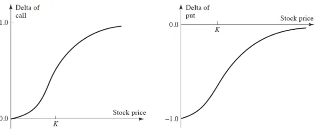
5.1 Delta variation of a put and a call option with respect to the underlying non-dividend paying stock price . . . 74

5.2 Theta variation of European call option along stock price . . . 78

5.3 Variation of an option’s gamma with respect to the underlying stock price . . . 81

5.4 Relationship between ∆Π and ∆Sin time ∆tfor a portfolio that is delta neutral with (a) slightly positive gamma, (b) large posi-tive gamma, (c) slightly negaposi-tive gamma, and (d) large negaposi-tive gamma. . . 84

5.5 Variation of an option’s vega with respect to the underlying stock price . . . 86

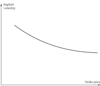
6.1 Volatility smile for equity options . . . 96

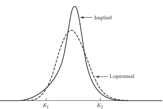
6.2 Implied distribution and lognormal distribution for equity options . . . 97

6.3 Volatility surface for European options on non-dividend paying stocks . . . 104

6.4 Variance rate expected path when (a) current variance rate is above long-term variance rate and (b) current variance rate is below long-term variance rate . . . 117

(9)

Abstract

This paper develops several methods to estimate a future volatility of a stock in order to correctly price corresponding stock options. The pricing model known as Black-Scholes-Merton is presented with a constant volatility parameter and compares it to stochastic volatility models. It mathematically describes the probability distribution of the underlying stock price changes implied by the models and the consequences. Arbitrage opportunities between stock options of various maturities or strike prices are explained from the volatility smile and volatility term structure.

(10)

Chapter 1 Introduction

Derivative instruments have existed since the eighteenth century in the United States of America but until recently, derivative contracts were not standardized, the markets were not regulated, and market participants had trouble buying and selling the contracts from the over-the-counter market on another more active secondary market.

The CBOE, Chicago Board Options Exchange, in 1973 decided to create an exchange for derivative options where the financial instruments started being traded with standard-ized strike prices and maturity dates. Derivatives traders could now engage or close out an option position at anytime, with lower transaction fees than before, to take their profits or limit their losses. The Options Clearing Corporation (OCC), acting as a third party in a derivative transaction, was created the same year in order to provide stability and financial integrity in the marketplace by ensuring that the obligations of the contracts are fulfilled. The exchange, providing liquidity and more opportunities for derivatives traders became a real success and similar markets quickly appeared around the world.

The multiplication of option exchanges and the increasing volatility in the financial markets encouraged traders to manage their portfolio’s risks. Interest rate risks, currency risks, and movements in financial instrument prices became a real concern to financial institutions, hedge funds, proprietary trading firms and other market participants, who still nowadays, spend a major time of their trading activities in managing their different market risk exposures. Risk management has become very sophisticated since then due to the apparition of the derivative products. A financial asset is called a derivative if its value is dependent on another financial asset’s price, which is called the underlying asset.

(11)

Many derivative products appeared to hedge the rising volatilities in the underlying markets. Financial institutions and market participants came up with new derivative in-struments like futures and forward contracts, swaps, warrants, options on stocks, on futures, on currencies, on stock indices, on commodities, and even more sophisticated contracts like credit default swaps (CDS), collateralized debt obligations (CDO), mortgage-backed secu-rities (MBS)... These financial innovations were an answer to the increasing risks in the underlying markets and offer market participants to reach their risk/profit ratio goals at lower costs.

This paper is focusing on one main derivative instrument: the stock options. Pricing stock options has become an important problem in the financial sphere and has attracted a lot of economists and mathematicians.

In 1900, Louis Bachelier suggested a stock option pricing formula in ”the theory of speculation”, the bases of which is the true assumption that stochastic process is followed by the stock prices. He assumed that Brownian motion is followed by the underlying stock having a drift rate equal to zero. However, his pricing formula was not really representing very well the real world of the stock option derivative markets. His model was giving the possibility of negative stock prices and the derivative options could price more than the underlying asset which is in theory not possible (see section 2.c. Arbitrage opportunities). Samuelson (1965) tried to improve Bachelier’s model by considering a geometric Brow-nian motion and computing the price of an option as the expected payoff actualized at a continuous rate, the drift of the option.

Then, Myron S. Scholes, Robert C. Merton and Fischer Black used the Itˆo’s lemma (a famous equation discovered by Kiyosi Itˆo in the 1940’s and 1950’s to model a continuous stochastic process) to solve the problem of option pricing on an underlying stock which is non-dividend paying. The pricing formula presented by Black-Scholes-Merton in 1973, drastically altered the financial world and is still nowadays used by traders and financial

(12)

institutions to correctly price a stock option derivative contract.

Based on more or less realistic assumptions (see section 4.p. The Black-Scholes-Merton model’s assumption), the model known as Black-Scholes-Merton has become popular due to the quick and easy computations that the model implies to generate a theoretical stock option price. The famous formula also introduced stochastic computations to the financial sphere to price derivative products. Nowadays, market participants use the model to value a stock option but also to determine the instantaneous implied volatility now, at a given point in time t, pricing an option at time t+ ∆t.

Devising a model to price derivative contracts has become a major challenge of the fi-nancial world and market participants are still waiting on the next pricing model that will be as easy as the Black-Scholes-Merton one but even more precise to the reality of the mar-kets. In the past few years, many mathematicians and physicians have worked to improve the Black-Scholes-Merton model to make it more realistic to the financial markets. Under-lying stock market’s jump-diffusion process, stochastic volatility of the underUnder-lying asset, a risk-free stochastic interest rate and other assumptions have been studied to enhance the model but always resulting in more complex mathematics and longer computations. With many complex models, is it really necessary to develop even more complex models for the purpose of representing the financial market’s trend in an improved way? In accordance with Stix and his book “A calculus of risk” (1998), 20% of losses that a trader suffers in the derivatives markets are due to a wrong estimation of parameters and pricing evalua-tion of the derivative products. This is the reason why mathematicians focus on finding a better model that will substitute the Black-Scholes-Merton one and will enable traders and financial institutions to lower the percentage of losses due to the mispricing estimations.

(13)

Despite the fact that the Black-Scholes-Merton model is the most popular nowadays, some market participants may use a different model or the Black-Scholes-Merton model maybe employed differently from what it was originally intended. This is the reason why it is very difficult to come up with a pricing model that can be used overtime. In fact, a valid pricing model today might not be working under the different market conditions tomorrow.

Derivatives traders and market participants are not all using the same model and have different estimations about future prices. This is why traders, market makers, financial in-stitutions and other market participants have different bids and asks for financial products. The outcome of all the bids is the quoted market price whereas the ask prices entered in the book order of the derivative contracts.

The best model will be the one that best represents the behavior of the derivatives markets and will last over time under all market conditions. Theoretical prices can be calculated quickly and easily with the least assumptions to be made and parameters to estimate. The quickness of the computation is really important in finance, as many traders must take decisions in real time. This is the reason why the Black-Scholes-Merton model, based on some more or less realistic assumptions, is such a success. The precision of the model is also an important factor as the amount of money traded in the derivatives markets is consequent. According to a study by marketwatch.com, there is between $630 trillion and $1.2 quadrillion ($1,200,000,000,000,000,000) invested in derivatives alone between the over-the-counter market and worldwide exchanges.

To get a theoretical option price on a stock that pays no dividends, if the traders use the model of Black-Scholes-Merton, they must implements some inputs in the pricing formula: the stock price underlying the option, the time taken before the option’s maturity date, option’s strike price to value, an interest rate which is risk free and constant, and underlying stock’s constant volatility over the option’s life span. The first four parameters

(14)

can be observed in the financial markets and therefore are known from traders. The only unknown parameter of the underlying stock that a trader must estimate is the future (or expected) volatility that will occur until expiration of the option.

A constant volatility level is assumed by the Black-Scholes-Merton model over the life of the option which is obviously not a realistic assumption but enables the computations of the model to be quick and easy. However, the model fails to explain many characteristics of the option derivatives markets such as the volatility smile. In fact, there are good reasons to believe that the underlying stock’s volatility is stochastic and derivatives markets to be more complex than Black, Scholes and Merton believe it to be.

Using a stochastic volatility model to price option contracts enables to have a more realistic representation of the underlying stock returns as a stochastic process involves the skewness and the kurtosis of a probability distribution. The lognormal distribution is assumed by Black-Scholes-Merton model for the underlying stock returns, which is not necessarily representing the real probability of the stock returns. In fact, the lognormal distribution has a tendency to underestimate a big positive or negative stock return while overestimating a small positive or negative return. However, with a stochastic volatility model, a trader can build a probability distribution for the underlying stock returns that better fits the reality of the underlying stock market as he can use an asymmetric distribu-tion, with lower or higher tails and with a lower or a higher peak. The trader, when using a stochastic volatility model, is also able to explain the volatility smile, which is not the case for a trader using the Black-Scholes-Merton model.

Therefore, as compared to the Black-Scholes-Merton model, stochastic volatility mod-els are more realistic as they describe the volatility smiles observed in the option derivatives markets in a more clear way. However, this type of models require more input estimations from a trader and therefore a higher chance for errors in pricing stock options. Stochastic volatility models as compared to the Black-Scholes-Merton model also require more

(15)

as-sumptions and are less time efficient.

This paper’s objective is to be able to determine and forecastT-month option’s future volatility with strike priceK from historical data and implied volatilities to correctly value a stock option and then be able to find arbitrage opportunities between options with dif-ferent strike prices and maturity dates.

This paper includes six chapters where chapter 1 and chapter 8 are the introduction and conclusion of the thesis respectively.

Chapter 2 is an introduction to the characteristics and the language of options. It de-scribes briefly some inequalities that a call option price must respect at anytime otherwise arbitrage opportunities appear in the option derivatives markets.

Chapter 3 is a description of the different volatilities that a trader must take into con-sideration when pricing options and a discussion that to predict the future volatility which volatility is the most appropriate to use.

Chapter 4 consists in building the Black-Scholes-Merton differential equation through a procedure studied which is led by stock price. Black-Scholes-Merton pricing formula proof and the put-call parity is given. Moreover, the Black-Scholes-Merton model applying to only European calls and puts on stocks that pay no dividends, a discussion on how to mod-ify the model to price American call furthermore put options on stocks paying dividends or not is included. Finally, the section ends up on a review of Black-Scholes-Merton model assumptions explaining why a stochastic volatility model might better reflect the reality of the option derivatives markets, since it is able to describe the volatility smile of the option contracts.

(16)

Chapter 5 talks about the Greek letters and how a trader can hedge his option portfolio to different market risks.

Chapter 6 is a presentation on how traders can estimate the future volatility from historical data and how they can determine the implied volatilities of the market. The volatility surface, volatility term structure, and volatility smile are then discussed in order to find arbitrage opportunities and determine the probability distributions of the under-lying stock returns associated with the volatility smiles. Different schemes to name a few the EWMA model, the GARCH(1,1) model and ARCH(m) model to estimate the future volatility of an underlying stock are presented.

Finally, chapter 7 is a presentation of the stochastic volatility models and the Monte Carlo simulation.

(17)

Chapter 2 Characteristics of an option contract

2.1 Option contract specifications

An option can be defined as a financial derivative mechanism which gives the right to the investor to purchase or sell an underlying asset’s particular quantity at a future date which is pre-determined (called as the option’s maturity date) at a particular price (known as strike price or exercise price), but is not an obligation on the investor to do so. The buyer of the option, in other terms, who is long the option, has the right to exercise the option when the maturity date is reached only if this one enables the investor to make a profit by exercising it. If this is not the case and exercising the option results in a loss for the long position, the buyer of the option will let the financial instrument expire and will lose the amount of money spent to purchase the derivative (called the premium of an option).

Now the other party, the option’s seller, who is short the option, will be forced to supply the underlying asset to the buyer if he decides to exercise the option at the maturity date. Thus, in case of a European option, the short position is totally dependent of the decision of the buyer and needs to be prepared to any possible scenarios at expiration of the derivative contract.

In American option case, the long position at any time earlier than the maturity date can exercise the option hence giving buyer more chances to show a profit on the contract overtime. This implies that at any time in the option’s life the short position should be ready to hand over the underlying asset as soon as it is decided by the long position to exercise the contract. Therefore, an American option as compared to European option

(18)

grants more power to the long position and less to the short position where to exercise the option or not is decided by the buyer only at the contract’s pre-determined maturity date. Hence, the premium of a European option should be lower than the premium of an American option having similar features.

Nowadays, majority of the options traded over-the-counter are European options how-ever, majority of the options that are traded publicly on exchanges are American options. Throughout this paper, we will implicitly consider all options to be European unless said otherwise.

There exists two types of options: a put option and a call option. A put option does not oblige but gives the right to sell a particular quantity of underlying asset at the ma-turity date at the exercise price. A call option does not oblige but gives the right to buy a particular quantity of the underlying asset at the strike price at the maturity date. The underlying asset of an option can vary. This can be a simple stock of a firm traded on an exchange, an index, a currency, a commodity or a future.

Options have become a popular financial instrument preventing investors from further losses in order to hedge a stock portfolio or by using these contracts as a real speculating investment by adding some leverage to an investment. No matter what way the investor purchases an option for, options are great tools to manage the risk of a portfolio and any investor must consider these types of contracts to get the best risk/reward ratio possible on an investment strategy.

2.2 Factors affecting the premium of an option

The premium of an option is dependent upon the volatility and the price of the un-derlying asset, the maturity date, the strike price and the risk-free interest rate which is equivalent to the similar time duration of the option’s life. For example, an investor will

(19)

use the 90-day Treasury bill rate in order to determine the premium of a 3-month call/put option.

2.2.1 Underlying asset price

An option’s premium can be seen as follow:

P remium option=Intrinsic value+T ime value

The intrinsic value is the value of an option if the contract would be exercised immediately. The option’s intrinsic value cannot be negative it can only be equal to zero or positive. Such as, a December 90 call for any prices of the underlying asset strictly above $90 will have a positive intrinsic value and an intrinsic value equal to zero for any prices equal to $90 or less. If we look at a June $50 put with the Facebook stock as the underlying asset, the option will have a positive intrinsic value for any Facebook stock prices strictly under $50, and equal to 0 if the stock price of the social media is $50 or more.

A call option and a put option with a positive intrinsic value are considered in-the-money. A put and a call are considered out-of-the-money if they have intrinsic value equals zero. A put and a call option where the price of the underlying asset is equal to the strike price of the derivative contract are considered at-the-money.

More generally, it is possible to come up with a formula for a put and a call intrinsic value.

intrinsic value for a put option : [K−S]+

intrinsic value for a call option : [S−K]+

where S represents the underlying stock price and K represents the option’s strike price. The graphs below show the intrinsic value (or payoff) and the profit & loss (“P&L”) curves for a long call, long put, short call and a short put option.

(20)

Figure 2.1: Intrinsic value and P&L from an option position at expiration

An option’s time value is characterized by the time quantity left earlier than option’s expi-ration and the probability that the contract will be in-the-money at maturity. The investor is willing to pay an additional cost to hold the contract as far there is a chance for him to make a profit by exercising the option. Thus, an option which is intensely out-of-the-money or intensely in-the-out-of-the-money will have a time value close to zero. The maximum time value of an option is achieved as at-the-money option. Indeed, there is a 50% chance to have a positive intrinsic value (K > S for a put, S > K for a call) and a 50% chance to have no intrinsic value (K < S for a put, S < K for a call). The time value, hence, of a financial derivative option is progressively growing as the option contract gets closer and closer at-the-money.

(21)

It is interesting to see that a call option which is in-the-money, the decreasing under-lying asset price gets closer to the option’s strike price, will have more time value but will also lose intrinsic value in the same time. On the other side, an in-the-money put option, the underlying asset price is increasing to get closer to the option’s strike price, would have more time value but will lose intrinsic value in the same time. In fact, as the call or put option is moving more towards in-the-money, there is a bigger chance for the option to be exercised at maturity and therefore it is not the willingness of the investors to pay the option’s time value where it would be more beneficial for them to straight away sell or purchase on exchange the underlying asset.

The price of an option, as observed from above, is a tradeoff involving time value and intrinsic value. A deeply in-the-money option will have as a result nearly zero time value and a positive intrinsic value. The option has little chance to be worthless before expira-tion and therefore does not hold any more time value. An deeply out-of-the-money opexpira-tion will have no intrinsic value and a premium which is low and equal to the time value. An at-the-money option premium will only hold an important time value.

2.2.2 Risk-free interest rate

As being long a call option involves paying a premium which is significantly less than buying directly the underlying asset, an investor can invest at the risk-free rate the dif-ference amount, through the option’s lifetime. This implies that if the risk-free rate is greater, it is better to buy the derivative option over the underlying asset and therefore the premium will increase.

Mathematically, the difference among the buying of the underlying asset and the ac-tualized call option strike price S −Ke−r(T−t) _{will get bigger as the risk free rate will}

(22)

When buying a put option, the buyer of the option will get from the sale of the under-lying asset the profits by using the put option at maturity instead of cashing out the sale of the underlying asset right away. A rational investor could invest the amount of the sale of the underlying asset at interest rate which is risk-free through the option’s life which is not possible for a buyer of the derivative instrument as he will have to pay a premium and wait until maturity to get money back. Thus, a put option represented by Ke−r(T−t)₋_S

will decrease in value as the risk-free rate will increase.

2.2.3 Lifetime of an option

When investing in option derivatives, the further the date of maturity of the option there is a greater chance that the long position will have to exercise his contract. In fact, the underlying asset price variations rises and the chances that the option will be exercised increases as the expiration date of the option is far in the future. The relationship between the maturity date and the price of a derivative contract is not linear. As time goes, the derivative instrument loses time value. At maturity, the option is only worth its intrinsic value or zero, but no time value is remaining in the option price.

2.2.4 Strike price of the option

If the strike price of a call option is low it has a better chance to be in-the-money at the time of maturity. Conversely, the higher the strike price, the lesser the probability for the call option to be exercised at expiration. However, for a put option, as the exercise price rises, the option has a greater probability to be in-the-money at expiration. The higher the strike price for a put option, the greater the chances that the put option will be exercised at expiration.

(23)

2.2.5 Volatility

The standard deviation of percentage change in the underlying asset prices calculated annually is called as the volatility. The long position of a call or a put is speculating on an increase or decrease in the underlying asset price. The higher premium is willingly paid by the trader while the volatility of the underlying asset is important as the option contract has better chances to be in-the-money at expiration. Thus, the more important the volatility, the higher the probability for the option to have some intrinsic value or being out-of-the-money, the higher the premium is.

The risk-free interest rate, the date of maturity, the strike price of an option and the underlying asset price are four factors that are used to determine the option’s premium by the investors in the financial markets. Then again, underlying asset volatility is unknown by investors as it implies for a trader to compute the underlying asset’s future volatility in the derivative contract’s life. Unfortunately, no one is able to forecast and predict the future and especially a future volatility of an underlying asset during a certain period of time of an underlying asset. This means traders need to use a fundamental and technical approach by using charts and graphs to best estimate the underlying asset’s future volatility.

It is very difficult to approximate the future volatility and requires traders to be as precise as possible. In fact, a wrong estimation of volatility will produce wrong option prices whose traders will not be able to take advantage of mispriced options.

With a total of five different factors, a trader is able to plug in the data in a theo-retical pricing model and estimate the right price of an option. The fact that traders get different prices for the same option contract is due to the volatility of the underlying asset that each trader must estimate. If a trader believes the financial markets are strongly efficient and reflect all public, private and inside information, “the best predictor of the future volatility ought to be the implied volatility. Just how good a predictor of future

(24)

volatility is implied volatility?” (Natenberg, 1994, p295). But a trader who agrees with the strong efficiency of the markets is not able to find any investment opportunities as he believes that options are correctly priced. Only traders with different opinions on the underlying asset’s volatility as compared to what the marketplace implies about volatility think options are mispriced. Traders are looking for mispriced opportunities between op-tions to sell the overvalued opop-tions and buy the undervalued ones. Therefore, traders are trying to come up with better volatility estimates than the implied volatility to implement in the pricing models and decide a trading strategy according to the mispriced instruments.

2.3 Arbitrage opportunities

Arbitrage is an operation which involves no cash outlay by the trader and will result in a sure profit for him. Arbitrage is inconsistent with the hypothesis of a strong efficient market as no sure profit or abnormal return is possible in this type of market when no risk is involved. In strong efficient markets, news are incorporated into prices right away and therefore no profitable arbitrage strategies are possible as the assets are instantaneously correctly priced. However, nowadays, arbitrage is frequently used by derivatives traders while searching for mispriced derivative instruments related to underlying assets or mis-priced derivative instruments between them.

To be able to find an arbitrage opportunity with a sure profit and no risk involved, an option must verify several conditions. The scenario where no dividend is paid by the underlying asset, a call option must satisfy all these conditions:

1. An option is a derivative financial instrument with limited risk. The maximum loss that a buyer of such instrument can endure is equal to the option value the investor paid for. Thus, an option premium cannot be negative: c≥0.

2. At maturity, if the option’s strike priceK is below the underlying asset priceST, the

(25)

the option has no intrinsic value and is worth zero: c=max(0, ST −K).

3. For a given time period τ, a call premium with strike price K1 must always be lower

than a call premium with strike price K2 if K1 > K2 : c(S, τ, K1)< c(S, τ, K2).

4. A call option premium cannot be greater in worth as compared to the price of the underlying asset. If it was so then the trader would have bought the underlying asset and not the derivative contract: c(S, τ, K) ≤ S. As negative premium of an option is not possible, the option will also be worth nothing if the price of the underlying asset is zero: c(0, τ, K) = 0.

5. c(S, τ, K) ≥ S −Ke−rτwhere τ is the elapse time between today and the date of maturity of the option and Ke−rτ _{is the actualized call option strike price. This}

inequality holds because a portfolio with a European call and a loan of amount K at maturity, the call strike price, is no less than the portfolio amount with one underlying asset at maturity.

These conditions also hold for underlying assets paying dividends but one modification must be done on the last condition number 5. Paying a dividend usually implies a decrease in price in the underlying asset by the same amount (at least in a strongly efficient market). If we suppose that investors know when the dividends are being paid, the last condition becomes c(S, τ, K)≥S−Ke−rτ ₋_Div_{. This inequality can be proved as follow: consider}

2 portfolios, one with a call c and a loan of amount K at maturity, the other with one underlying asset and a loan equal to the dividend amount. At any time between the present moment and call option expiry date, the call option with the loan of amount K at option expiration date portfolio is worth the same or more than the second portfolio.

(26)

Chapter 3 Volatility

Volatility can be described as the percentage changes underlying contract prices. The parameter for the volatility can be seen as a mix of negative and positive rates of return. In mathematical terms, the volatility of an instrument is characterized by the standard deviation and gives no information about the direction of the movement.

When computing the theoretical option value using the Black-Scholes-Merton model, we take volatility as an input which is unknown and therefore traders must estimate this data. Volatility is an important factor, if not the most important, in price determination for the option. The well-known theoretical pricing model, Black-Scholes-Merton, takes volatil-ity as a constant which implies the underlying asset will have the same volatilvolatil-ity during the entire life of the option but in reality, it is more appropriate to describe volatility as a stochastic process. The constant volatility assumption over the life of the option is for simplicity and quick computation of theoretical values.

To best estimate the volatility of an option, traders use the historical volatility and the implied volatility given by the marketplace. The volatility factor is the hardest factor to estimate but the more crucial in evaluating option theoretical values, as these derivative contracts change quickly with changes in volatility. Commonly this is known as the volatil-ity input that each trader uses in the model, which gives the trader an idea if the option is overvalued or undervalued.

A trader who anticipates a higher volatility than the implied volatility will buy the options that he believes are undervalued, hoping the marketplace will match the trader’s

(27)

volatility estimate before the expiration of the options. The trader will therefore profit by selling back the options once the implied volatilities are equal to his estimations. In the case where a trader anticipates a lower volatility than the implied volatility, the trader will find out that options are overvalued and will start selling options. The trader will realize a profit if the implied volatility starts declining to reach out the trader’s volatility estimate before the expiration of the options. This is why nowadays, traders in the pit at the Chicago Board Options Exchange (CBOE) do not talk about buying or selling options anymore but buying or selling volatility instead. Thus, traders find overvalued and undervalued options as they come up with different volatility estimations than the ones in the marketplace to then buy and sell the volatility. The more precise the estimation of the volatility, the better the evaluation of the theoretical value of the option.

3.1 The different types of volatilities to consider

3.1.1 Future volatility

The volatility that each trader is interested in knowing since this information helps the traders to decipher and get a theoretical price for the option is the future volatility. The future volatility represents the price changes of the underlying contract in the future till the option expiration date is reached. Future volatility is not known by any trader but they all try to best estimate it.

3.1.2 Historical volatility

Derivatives traders also commonly call historical volatility as realized volatility. When traders try to best guess the future volatility, one possibility is to refer to historical data and see the different price changes of the underlying market in the past. No trader can assume that past volatility will be identically reproduced in the future but this is a great way to start estimating the future volatility. In fact, suppose volatility of an underlying contract for the last five years, has been in the range [10%, 30%] constantly. An estimation

(28)

for the future volatility of the underlying contract out of this range would hardly make sense. An approximation in the past years range of 10% and 30% is more likely to be true even though it has the exact same probability for the future volatility to be within the defined interval or not.

To calculate the historical volatility of an underlying contract, various ways can be employed but each way depends on two parameters: the past time span over which to compute the volatility and the elapsed time among consecutive movements in price. For example, a trader can analyze the 10-day underlying asset’s return during a period of five years or a 6-month underlying asset’s return during a period of ten years.

Longer periods give an average of the past volatility while shorter periods reveal un-usual and extreme characteristics about the past volatility. Thus, to fully examine the past volatility, a trader must compare wide variety of scenarios with different time periods and intervals between data. Surprisingly, the interval chosen by the trader does not seem to impact a lot the final result about the historical volatility. In fact,“a contract which is volatile from day to day is likely to be equally volatile from week to week, or month to month” (Natenberg, 1994, p70) but at the end the different data seem to exhibit one general volatility trend and level.

The historical volatility is given by the standard deviation of the return of the un-derlying asset prior to the option contract issuance. Suppose we omit the dividends, the underlying asset’s return can be computed as follow

RT =

ST −St St

= dS

S

(29)

such as

dS

S =µdt+σdv

where dv is a Wiener process. This means the variable dv is following a normal law with variance dt and mean equal to zero. This is equivalent to say that RT is following a

lognormal law or ln(1 + RT) follows a normal law. A major assumption of the

Black-Scholes-Merton model is this, where “price percentage changes are assumed to be normally distributed, the continuous compounding of these price changes will cause the prices at maturity to be lognormally distributed” (Natenberg, 1994, p62-63). Further explanations about the Brownian motion of the underlying asset instantaneous return which is geometric in nature and the lognormally property are given in section 3.b. The process for a stock price, and 3.d. The lognormal properties of stock prices.

This gives the reason why lesser strike price option is cheaper than an option with a higher strike price, where both strike prices are an equal amount away from the underlying instrument price. For example, assume trading is done at $100 for an underlying contract and presume the prices of the underlying contract are normally distributed. As a result, the 90 put and 110 call should have theoretical values which are equal as the two are being out-of-the-money by 10%. Yet, with a lognormal distribution assumption in the Black-Scholes-Merton model, the 90 put will be less expensive as compared to the 110 call. From this observation it can be concluded that a higher upside price movement is allowed by the lognormal distribution as compared to the downside price movement hence there is better chance for 110 call to be in-the-money than the 90 put.

The historical volatility in reality, is not constant as the Black-Scholes-Merton model supposes so, but rather follows a stochastic process. In fact, the historical volatilities of one underlying asset are going to be more or less important at moment t, varying over time, but the Black-Scholes-Merton model will use one volatility constant which best describes the historical movements of the underlying asset.

(30)

3.1.3 Forecast volatility

Forecast volatility is an attempt to estimate for an underlying contract the future volatility in the options life span. Common options have expiration dates in 3, 6 or 9 months. Some services, technicians, proprietary trading firms or hedge funds try to fore-cast volatility for periods similar to common options in the marketplace.

3.1.4 Implied volatility

Establishing upon underlying contract historical volatility and then computing the fu-ture volatility has been criticized and every investor is aware that past figures do not predict future figures. This is why traders must use the historical volatility of an underlying con-tract as a constructive technical indicator. In fact, traders do not blindly and exclusively use this tool to make trade decisions but they do use it to help them make trade decisions combined with other factors, such as implied volatility and news catalyst.

Traders analyze option prices in the marketplace and deduce the volatility which is employed by the theoretical pricing model known as Black-Scholes-Merton by iterating the pricing formula. The volatility determined by the marketplace is called implied volatility. In other words “the implied volatility is the volatility we must feed into our theoretical pricing model to yield a theoretical value identical to the price of the option in the marketplace” (Natenberg, 1994, p72). As the implied volatility is based on the present value of the market, it is a better estimator than the historical volatility. The main idea is that the base for the implied volatility is the options present prices which include future events. It should be noted that implied volatility is subject to change overtime as option prices in the marketplace and market conditions are constantly changing.

(31)

Implied volatility has a major drawback that it assumes a diffusion process of the underlying contract. This diffusion process for the underlying asset, in the case of the Black-Scholes-Merton model, is Brownian geometric which does not really well represent the reality. A diffusion process implies price changes are continuous and smooth, with no gaps between consecutive prices. A good example to describe a diffusion process is the temperatures in one location. The temperature might increase from 70F to 73F but for a very small period of time in the middle, the temperature reached 71F and 72F. However, is a diffusion process really representing well price changes in the marketplace? In fact, prices might also follow a jump process. This means prices can jump to new prices overtime without reaching intermediate values.

Most of the theoretical pricing models, whose Black-Scholes-Merton one, assume that prices follow a diffusion process which can be pretty accurate when we look at the trading sessions, prices change with no gaps. However, between two trading sessions, it is common that an underlying contract closes at a particular price and opens at another price the next morning. Even during the trading sessions, an illiquid underlying contract can be subject to a jump process. Thus, the diffusion process assumed by the models make them convenient and easy to use but these models do not truly correspond to the reality as financial markets rather follow a jump-diffusion process.

Few pricing models have been developed assuming a jump-diffusion process in the financial markets but they are not very used by traders due to the fact that they are math-ematically more complex and require more inputs, which means more estimations to do and therefore more chances to make mistakes in evaluating the parameters.

Traders do rely on the implied volatility given by the marketplace and particularly pay more attention to the options which are at-the-money as they respond more quickly to volatility changes than any other options (highest vegas are owned by at-the-money options) hence they are better predictor of the future volatility. This method using implied

(32)

volatilities to forecast volatilities of underlying contracts is the most commonly used among traders. They use numerical schemes and programs (like the Newton-Rhapson algorithm or by interpolation) to revert the pricing models and deduce implied volatilities and predict future volatilities.

In the literal sense premium is the option price, traders among each other use the word “premium” for referring to implied volatility. This makes more sense as the option price is primarily dependent on the underlying contract volatility characteristics. Thus, traders might say premiums are high meaning the implied volatility is high which is equivalent to a high price for the corresponding option.

For example, suppose a 105 call with $0.96 as the theoretical value and a price of $1.34 in the marketplace. The basis for the theoretical value is 16% volatility (the volatility estimate by the trader) whereas the basis for the price is 18.5% volatility (which is the implied volatility). It will be mentioned by the traders that the option being overpriced in terms of volatility rather than dollar value. Thus, traders rather see the 105 call option as being 2.5% overpriced than $0.38 overpriced.

Once a trader is able to find out by iterating the Black-Scholes-Merton model the implied volatilities, a comparison can be drawn between the implied volatilities and the forecast volatilities to deduce if options are overvalued or undervalued. If implied volatil-ities are low with respect to forecast volatilvolatil-ities, the trader will prefer to buy options as they will appear to be underpriced. If implied volatilities are high with respect to forecast volatilities, the trader will prefer to sell options as they will look overvalued. Thus, the intelligent trader will take an appropriate trading strategy to play the overpriced and un-derpriced options by remaining delta neutral during the time of his investment.

(33)

3.1.5 Seasonal volatility

Another volatility kind that traders must take into consideration when investing: the seasonal volatility. This particularly affects commodity traders but also other investors dealing with stocks, futures and other instruments. For example, stocks and futures can be very sensitive to volatility factors coming from the season of companies’ results. However, the most subject to seasonal volatility are commodities like soybean, gold, wheat, corn where price changes can vary by a lot due to extreme weather conditions. This is why some commodity traders assign higher volatilities during certain time of the year due to events sharply affecting commodity prices and rising price movements.

3.2 Volatility revisited

As we have seen several interpretations for volatility done by the traders, theoretically speaking, the option value primarily depends on the underlying contract volatility which occurs over the option’s life span. Some important characteristics about volatility are worth to be notifying.

Volatility, just like prices of the underlying contract, can rise and fall. In fact, if we look at the volatility index (also called the fear index or the VIX) traded on the CBOE, Chicago Board Options Exchange, the VIX quoted 13.96 on April 26,2016, then reached 16.05 on May 4 2016, to then decreased to 13.63 on May 10, 2016. But unlike underlying contract prices, which are apparently not bounded and can move in either direction freely, it is likely to have “an equilibrium to which the volatility always returns” (Natenberg, 1994, p273). Indeed, volatility seems to be bounded and fluctuates into a defined interval. Thus, volatility always seems to reverse and erase previous rise or fall. Therefore, one way to estimate volatility of an underlying asset may be finding a volatility equilibrium which has variations below and above in comparable amounts around this equilibrium. In this case, we say that volatility is mean reverting.

(34)

This means that if the volatility is higher than the volatility average, the trader can safely assume that it will go down to its mean value, and if the volatility is below the mean volatility, it is safe to assume by the trader that it will go up to its mean value. Hence volatility fluctuates around its mean value.

Volatility also expresses some trend characteristics. For example, there was an upward trend in the VIX during the month of April 2016 or a downward trend during the period February-March 2016. Moreover, during these major trends, the volatility showed some small fluctuations since volatility decreased and increased in shorter time spans.

As volatility forecast remains a difficult exercise and are often incorrect, traders might approach the problem differently and take a more general approach. Rather than trying to figure out the correct future volatility, a trader may look at the volatility environment in the financial markets and try to find the right strategies corresponding to current volatility climate. For this, a trader must be able to answer several questions like what is the historical trend regarding volatility and historical implied volatility?, what is the stability of the volatility?, what is the underlying contract volatility long-term mean?

Consider for instance that a trader wants to invest in a 3-month to expiration option and tries to coordinate an appropriate volatility strategy. The trader will look at historical volatilities and historical implied volatilities over the past 3-month to determine a coherent strategy. If the historical volatility is declining and is higher as compared to the mean in the long-term, or there is a rise in the historical volatility and is under the long-term historical mean, the trader has some good basis to assume that the volatility eventually reach the long-term historical volatility mean at one point by either rising or falling. At the same time, if the historical implied volatility has a similar trend than the historical volatility, all indicators seem to perfectly indicate a path for the future volatility.

Scenarios are not always this simple in the real life. Historical volatility trends might be in contradiction with historical implied volatilities and this is pretty frequently that a

(35)

trader needs to face situations where the historical volatility is higher than the long-term historical mean and falling whereas the historical implied volatility is increasing, or his-torical volatility is higher (or lower) as compared to the long-term mean furthermore it is increasing (or decreasing). In these situations, the trader is unlikely to have a strong degree of confidence in his volatility estimation as some indicators point out one kind of strategy and the others point to a different type of strategy.

Let’s look at a concrete example on how a trader could deal in this type of situation. Suppose a 6-week option and a 19-week option are available in the marketplace. Both the historical volatility and implied volatility for the 6-week option are well above the long-term mean volatility and seem to keep increasing. In the case of the 19-week option, the current implied volatility is higher as compared to the historical volatility which is greater than the mean for the long-term volatility. A trader might get confused by having these kind of contradictory signals as to whether one should sell or purchase the volatility for both options. Nevertheless, a much more acceptable risky strategy called time spread will be devised by the trader. In this case, there is more probability that the volatility for the 19-week option will revert to its mean than the 6-week option therefore the trader would rather short the volatility in the 19-week option than the short-term option. At the same time, the trader could long the 6-week option and would therefore be hedged along a rising volatility continuously over the next 6 weeks of the underlying contract.

By selling the long-term option and purchasing the short-term option, the trader is taking a position with acceptable risk characteristics. The trader’s position will not be without risk as if historical volatility falls below its long-term mean or reaches it and im-plied volatility remains high, the position will show a substantial negative theoretical edge. However, the trader attempted to pick a right strategy that fits his market conditions with an acceptable margin for error and tried to get the best risk/theoretical edge ratio possible.

(36)

3.3 Implied vs historical volatility

Implied volatility reflects a consensus volatility among all market participants con-cerning the underlying contract future volatility in the option remaining life span. As traders expect more fluctuations in the underlying contract, the implied volatility rises; as traders expect fewer fluctuations in the underlying contract, the implied volatility de-creases. Market traders assume that the historical volatility is a good data to predict what will happen in the future and therefore a changing historical volatility in the underlying as-set will conduct traders to modify the implied volatility. “However, fluctuations in implied volatility are usually less than fluctuations in historical volatility” (Natenberg, 1994, p290).

Moreover, the further the expiration of the option, the more likely the underlying contract volatility will move back to its mean value. This explains why long-term options have forecast volatilities closer to their long-term historical volatility means than short-term options where the forecast volatilities can sometimes be quite different from the long-term mean depending on the market conditions. Thus, as long-term options have a stronger mean reverting characteristic of volatility compared to short-term options, the short-term options implied volatility will rise more as compared to the implied volatility of long-term options. In the same case, if historical volatility falls, the implied volatility of short-term options will decline more as compared to the long-term options implied volatility. Hence, it can be concluded that the main factor affecting long-term option implied volatility is the historical volatility of the underlying contract while significant events and news, affecting the underlying contract to become more volatile, will play a bigger role in the short-term options implied volatility. This is why for short-term options, it is not rare to see an implied volatility which is less correlated to the historical volatility. In some cases, the implied volatility and historical volatility can even give contradictory results to the market traders.

(37)

For example, if the marketplace is aware of chances that some important events will take place in the future, there can be an increase in the implied volatility even though historical volatility may have been low comparatively. This is a reason why traders see the implied volatility to drastically drop after an event has happened as all the uncertainty about the event has been removed from the market.

3.4 Implied vs future volatility

As truly believed by several traders, all the information available which affects the underlying asset value is reflected by the price and therefore traders believe that the implied volatility of options should be the best estimation of the future volatilities. But how good is the implied volatility of an option predicting the future volatility?

Once options have expired, traders may look back to the historical implied volatili-ties and compare them with the real volatilivolatili-ties that actually occurred over the option’s life span to assess how accurately the implied volatility of an option estimates the future volatility. By doing this experience several times, traders have come up to a conclusion. When expiration of the option is relatively far in the future, the future volatility is much more stable than it is with few days remaining before expiration of the derivative contract. “This is logical as if we recall the mean reverting characteristics of volatility are much less certain over short periods of time than over long periods” (Natenberg, 1994, p295). In fact, with less days left until expiration a major change in the underlying contract will lead to volatility rising sharply while on the other hand, a quiet underlying asset which sits still in the last few days before expiration in life of an option will cause a sharp drop in volatility. Thus, a trader will act differently according to the amount of time remaining to the option’s life.

The trader is aware that volatility is more stable when considering a longer period of time and therefore implied volatility is relatively stable. As expiration approaches, the

(38)

volatility of an underlying asset can become very unstable and the implied volatility can be subject to a lot of fluctuations. The main idea here is that market traders try to avoid short-term bad luck.

With a considerable time remaining to expiration, a trader is aware that many events which can affect the underlying asset’s volatility differently will compensate between each other giving as a result a relatively stable implied volatility for an option expiring in a long period of time. However, with few days left before expiration, only a limited number of future events affect the implied volatility of the derivative contract giving the restricted number of events an important impact on the implied volatility of the option. One impor-tant negative event with few days left to expiration of the option will dangerously impact the trader’s strategy as the volatility will move in the opposite direction of the trader’s estimation: this is short-term bad luck.

3.5 Conclusion

A trader who has been involved in investing in stocks at the beginning of his career might wonder why the volatility factor is so important in option trading. He probably has been trading and betting on the direction of stock prices and indexes where volatility was not as much a consideration as in option trading. The stock trader is aware that he can pursue some directional strategies in the option market (by being long or short delta) and questions why traders bother with volatility rather than the direction of option premiums. This is due to the fact that traders find simpler to predict volatility rather than forecast market directions.

Moreover, volatility strategies can offer substantial profits and offer a better risk/reward ratio than directional strategies by reducing the trader’s risk exposure.

Changing a volatility assumption can lead to drastic effects on options value. In fact, at-the-money options will suffer the highest variation in terms of dollar amount while the

(39)

most quickly responding to a change in volatility assumption in terms of percentage change will be the out-of-the-money options.

Given the importance of a good estimation of the volatility, traders spend a considerable amount of time determining the volatility. Gathering all information from the different volatilities previously seen, the intelligent trader will be able to take a smart decision on his final volatility estimation.

The trader will look for option trading strategies with high risk/reward ratio, and which do not result in a catastrophic loss if his volatility estimation is wrong. A trader must always consider the possibility of error and because predicting volatility remains a difficult task, the trader will pick strategies having margin for error higher as compared to rest. It is not possible for a trader to carry on for a long time if his positive theoretical edge disappears when the volatility turns out to be slightly different from his volatility estimations.

Finally, every market has its own volatility characteristics and a trader must not gen-eralize any of these characteristics and apply them blindly to each market. An intelligent trader will mix the technical characteristics of volatility with each feature of volatility of a given market (foreign currencies, interest rates, commodities, futures, stocks) to take a final decision.

(40)

Chapter 4 The Black-Scholes-Merton model

4.1 Introduction to generalized Wiener processes

A stochastic process can be defined as changes in value of a variable in an unpredictable way over time. Stock prices in the financial markets are following variable, discrete-time stochastic processes as they can take discrete values only (since stock prices are given in cent multiples), and price changes can occur only during trading hours on the exchange. However, it can be very practical for many purposes to assume that stock prices follow a continuous-variable (within a defined interval the stock price may assume any value), continuous-time (the stock price can change in value at any time) stochastic process. In fact, this process can be useful to understand the pricing of options and other derivatives instruments.

A Markov process is a stochastic process type in which for future value prediction, only the current value of variable is required. The variable’s past values and how the present value has emerged is deduced using the past values is not of interest. Markov process is followed by stock prices. For instance, let the price of Apple stock be $97. A stock trader who tries to predict the future direction for the Apple stock should not consider the past prices of the Apple stock that occurred in past one week, month or year but should rather focus only on one relevant information which is the current stock price $97.

As the stock trader cannot be certain about his future stock price predictions, he must express a probability percentage for each predicted possible outcome. As future stock prices are independent from past prices, the Markov process is the most realistic probability distribution for stock prices as it implies no relationship between past and future data.

(41)

A special type of Markov stochastic process is called Wiener process which has a vari-ance rate of 1 per year and mean change of zero. A Wiener process is followed by variable v if:

• the change ∆v during a small time period ∆t is ∆v =√∆t

• the values of ∆v for any two different intervals of time, ∆t, are independent

Hence using the Wiener process definition, the variable ∆v has a normal distribution with

mean of ∆v = 0

variance of ∆v = ∆t

and Markov process is followed by it.

Take into consideration the change variable value v over long period of time T =

v(T)−v(0). It can be observed as the aggregate of variable value changes in N small intervals each having a length of ∆t where

N = T ∆t v(T)−v(0) = N X i=1 i √ ∆t

where i (i=1, 2,..., N) are distributed φ(0,1) and are independent between each other (definition of a Wiener process). Obviously, the smaller ∆t, the more precise the variable value v changes can be observed. Saying other way round, as ∆t→0, the more intervals N we have and a better detailed representation of the changes in variable v value is achieved.

(42)

Hence, the time period T =v(T)−v(0) has a normal distribution with

mean of [v(T)−v(0)] = 0

variance of [v(T)−v(0)] =N∆t =T

For example, suppose a variable v that follows a Wiener process. Assume thatt0 = 25

years. This means that at the year 1 end, the variable v value is distributed normally having a variance of 1 and a mean of 25. At 10 years end, it is still distributed normally with a variance of 10 and a mean of 25.

A stochastic process can be defined by a variance rate and a drift rate. The variance rate is the variance per unit of time whereas drift rate is the mean change per unit of time. A Wiener processdv =adtin stochastic calculus is equivalent to ∆v =a∆t in the limit as ∆t→0. Explored uptill now, the Wiener processdv has a variance rate of 1 and a drift rate of zero. A zero drift rate implies that at any future time, the variable v expected value is equal to the current value which is zero. The meaning of variance rate equal 1 is that in a time interval T, the variance for the variable v is equivalent to T. A Wiener process, in general form, for a given variable x in terms ofdv is presented as

dx=adt+bdv (4.1)

where a and b are constants.

Let’s focus on the equation (4.1) of Wiener process in a general form. The variable x

has an expected drift rate given by a per unit of time is shown by the termadt. Thus, the variable x rises by the quantity aT in a period of time T. To add the effect of variations or noise to the trajectory of variable x, the bdv term is added. Thus, the noise present is

(43)

equal to the product of b and the Wiener process dv. Wiener process dv has the variance rate per unit time equals 1, hence, bdv has a variance rate b2 per unit of time. Change in value of the variable x, is given by ∆x, over a small interval of time ∆t

∆x=a∆t+b√∆t

where has a standard normal distribution and ∆x has a normal distribution with

∆x mean=a∆t

∆x variance=b2∆t

An Itˆo process is classified as a general form of Wiener process in where the parametersa

andbare functions of timetand the underlying variablex. This implies that the Itˆo process variance rate and expected drift rate are subject to change over time. Mathematically, we can write an Itˆo process as below

dx =a(x, t)dt+b(x, t)dv

This Itˆo process can be classified as a Markov process since the changes at a given time

t in variable x are dependent solely on the value of x at that particular time t, and does not use the value of x at previous times. In a small interval of time from t to t+ ∆t, the change in variable xis given from x to x+ ∆x where

∆x=a(x, t)∆t+b(x, t)√∆t (4.2)

4.2 The stock price process

A stock price does not follow the general form of Wiener process which has constant variance rate and expected drift rate as it fails to take into account stock prices’ one

(44)

important element. The missing element is known as the expected required rate of return which is not dependent on price of stock.

For example, if expected return per year required by a trader is 12% when the stock prices $15, the same rate of return will be required when the stock price increases to $50 given the market conditions remain the same. Therefore, the assumption that expected drift rate is constant is not correct, a better assumption is that the expected return is constant which equals the expected drift rate ratio stock price.

LetS be the stock price at a given timet, the expected drift rate inS can be seen asµS

whereµis the expected rate of return parameter which is constant. Hence, in a small time duration ∆t, the increase expected inS equalsµS∆t. Let’s assume there is no uncertainty or variability about the expected return (b = 0), the generalized Wiener process equation becomes ∆S=µS∆t In the limit, as ∆t→0 dS =µSdt which is equivalent to dS S =µdt

Integrating above equation with limits given by time 0 and time T, the following equation is derived

ST =S0eµT

where the stock price at time 0 and time T are given by S0 and ST respectively. Thus,

with no uncertainty, the continuously compounded growth rate for stock price isµper unit of time. There is some uncertainty in reality. It is right to assume that the variation in percentage return over a short time duration ∆t is same independent of the stock price.

Option Volatility & Arbitrage Opportunities

Louisiana State University

LSU Digital Commons

Option Volatility & Arbitrage Opportunities

Mikael Boffetti

&

Acknowledgments

Table of Contents

List of Tables

List of Figures

Abstract

Chapter 1

Introduction

Chapter 2

Characteristics of an option contract

2.1

Option contract specifications

2.2

Factors affecting the premium of an option

2.2.1

Underlying asset price

2.2.2

Risk-free interest rate

2.2.3

Lifetime of an option

2.2.4

Strike price of the option

2.2.5

Volatility

2.3

Arbitrage opportunities

Chapter 3

Volatility

3.1

The different types of volatilities to consider

3.1.1

Future volatility

3.1.2

Historical volatility

3.1.3

Forecast volatility

3.1.4

Implied volatility

3.1.5

Seasonal volatility

3.2

Volatility revisited

3.3

Implied vs historical volatility

3.4

Implied vs future volatility

3.5

Conclusion

Chapter 4

The Black-Scholes-Merton model

4.1

Introduction to generalized Wiener processes

4.2

The stock price process