A Case Study in a Recommender System Based on Purchase Data

(1)

A Case Study in a Recommender System Based on

Purchase Data

Bruno Pradel

Université Paris 6 Paris, France

Savaneary Sean

KXEN Europe Suresnes, France

Julien Delporte

INSA de Rouen Saint-Étienne-du-Rouvray, France

Sébastien Guérif, Céline Rouveirol

Université Paris-Nord Villetaneuse, France

Nicolas Usunier

Université Paris 6 Paris, France

Françoise Fogelman-Soulié

KXEN Europe Suresnes, France

Frédéric Dufau-Joel

La Boîte à Outils France

ABSTRACT

Collaborative filtering has been extensively studied in the context of ratings prediction. However, industrial recom-mender systems often aim at predicting a few items of im-mediate interest to the user, typically products that (s)he is likely to buy in the near future. In a collaborative filtering setting, the prediction may be based on the user’s purchase history rather than rating information, which may be unreli-able or unavailunreli-able. In this paper, we present an experimen-tal evaluation of various collaborative filtering algorithms on a real-world dataset of purchase history from customers in a store of a French home improvement and building supplies chain. These experiments are part of the development of a prototype recommender system for salespeople in the store. We show how different settings for training and applying the models, as well as the introduction of domain knowl-edge may dramatically influence both the absolute and the relative performances of the different algorithms. To the best of our knowledge, the influence of these parameters on the quality of the predictions of recommender systems has rarely been reported in the literature.

Categories and Subject Descriptors

H.3.0 [Information Storage and Retrieval]: General; H.2.8 [Database Applications]: Data Mining

General Terms

Experimentation, Algorithms, Performance

Permission to make digital or hard copies of all or part of this work for personal or classroom use is granted without fee provided that copies are not made or distributed for profit or commercial advantage and that copies bear this notice and the full citation on the first page. To copy otherwise, to republish, to post on servers or to redistribute to lists, requires prior specific permission and/or a fee.

Keywords

Recommender Systems, Collaborative Filtering

1. INTRODUCTION

Systems for personalized recommendation aim at predict-ing a few items (movies, books, ...) of interest to a particular user. They have been extensively studied in the past decade [2, 17], with a particular attention given to the collaborative filtering (CF) approach [18, 24]. In contrast to content-based recommender systems, collaborative filters rely solely on the detection of interaction patterns between users and items, where an interaction can be the rating or the pur-chase of an item. For instance, a system can recommend to a target user some products purchased by other users whose purchase history is similar to the target user’s, making rec-ommendation possible even if relevant descriptions of users or items are unavailable.

The development of collaborative filters has followed sev-eral, mostly independent directions. The first direction, which accounts for the majority of works in CF, is the de-velopment of different types of algorithms, such as memory-based techniques, matrix factorization algorithms, proba-bilistic models and ensemble methods [18, 24, 6, 14]. Al-most all of these works have focused on ratings prediction on publicly available benchmark datasets such as MovieLens1 or NetFlix2. A second direction is the identification of do-main dependent variables that describe interactions between users and items and which may influence the recommenda-tion performance. For instance, purchase time can be used to take into account the recency of past customer purchases for the recommendation [7, 15]. Another example is contex-tual variables such as the intent of a purchase (e.g. whether a book is purchased for personal or professional purposes), which allow to perform situated recommendations of poten-tially greater accuracy [1, 3, 5, 19]. These works gener-ally focus on the impact of introducing domain knowledge,

1

http://www.grouplens.org/node/73 2_{http://www.netflixprize.com/}

(2)

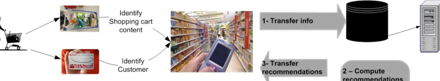
Figure 1: Vendors in the store use a PDA which is equipped to read product bar-codes and loyalty cards. An application has been developed to receive recommendations.

and have often been evaluated on medium-scale proprietary purchase datasets with very little emphasis on performance comparisons between algorithms.

The abundance of academic papers on CF should be con-trasted with many critical aspects of the design of com-mercial recommender systems which remain mostly undoc-umented. A data miner who wants to build a recommender system has to choose the appropriate algorithm to use, and probably incorporate domain knowledge to increase the rec-ommendation quality. However, for many retailers, rating data is unavailable, or may be unreliable because ratings are purely declarative. Personalized recommendations should then be based on the customers’ purchase history or other kind of implicit feedback, which is a different type of data because it does not containnegative feedback[10]: high and low ratings inform us about what a user likes and dislikes, but past purchases do not reliably inform us about the prod-ucts which will not interest the customer in the future. The choice of the best algorithm becomes an issue as most collab-orative filtering algorithms have been compared and studied in depth only on rating data. Moreover, since the algorith-mic dimension is often studied independently of the intro-duction of domain knowledge, the relative and joint impact of these two parameters on the recommendation quality is mostly unknown.

In this paper, we present a case-study on CF recommender systems using a dataset containing the purchase history of more than 50,000 loyal customers of a home improvement store over 3 years, containing about 4.6 million transactions. We systematically evaluate three families of CF algorithms, namely item-based recommendation [16], matrix factoriza-tion [14, 26, 20] and associafactoriza-tion rule mining algorithms [22, 11] on various settings in which we introduce increasing amounts of domain knowledge. In our case, domain knowl-edge is inferred from purchase data in which we identify

high purchase activity periods of the customers. This leads us first to consider the recency of the purchases in a cus-tomer’s history as a critical parameter, and secondly to a clustering of the high purchase activity periods, where the categories have a meaningful interpretation in terms of con-textual variables. Our main results are:

• The blind application of the algorithms leads to very low performances, which are unacceptable for an in-dustrial recommender system. The influence of in-corporating domain knowledge in the recommendation process has already been reported in the literature, even for the task of ratings prediction [13] where taking into account the changes in user tastes over time im-proves performances. Domain knowledge is even more

important for short-term recommendation (as in our case) since the prediction task is more difficult.

• The difference in performance between the various al-gorithms is very small compared to what can be gained by introducing context in the recommendations. These results provide additional evidence for the need of context-aware recommender systems, in line with recent works [5, 19].

• Matrix factorizations algorithms and item-based tech-niques detect slightly different patterns between cus-tomers and items, as was already noticed in the con-text of ratings prediction [12]. On our purchase data, this leads factorization methods to mostly recommend best-sellers while item-based CF, like association rules, tends to recommend more products that are rarely bought.

• Surprisingly, the most accurate recommendations on our data are given by the simplest form of bigram association rules. This contrasts with the results on rating data where memory-based and matrix factor-ization are among the best performing methods [6, 14] and association rules are almost never used.

The paper is organized as follows. In Section 2, we present the dataset and the original recommendation task which lead to this study. We then describe our experimental protocol and the algorithms we evaluate in Sections 3 and 4 respec-tively. The results of an approach which uses no domain knowledge are reported in Section 5. We show the impact on the performance of a more business-oriented modeling in Section 6. Finally, Section 7 concludes the paper.

2. RECOMMENDATION TASK AND DATASET

This study is motivated by a need for an automatic recom-mender system, expressed by a French retailer, La Boˆıte `a Outils3(BAO). The company possesses 27 medium and large size stores in the South-East of France, and sells products for home improvement. BAO wants to equip salespeople in the stores with tools helping them provide their customers with better and more professional answers. Very often, cus-tomers come to the store and leave, without noticing they forgot some products they will need for the job they have in mind. After that, they start working and realize they have to come back, or try a closer competitor’s store. BAO thus wants to help the salespeople make sure that the customer

(3)

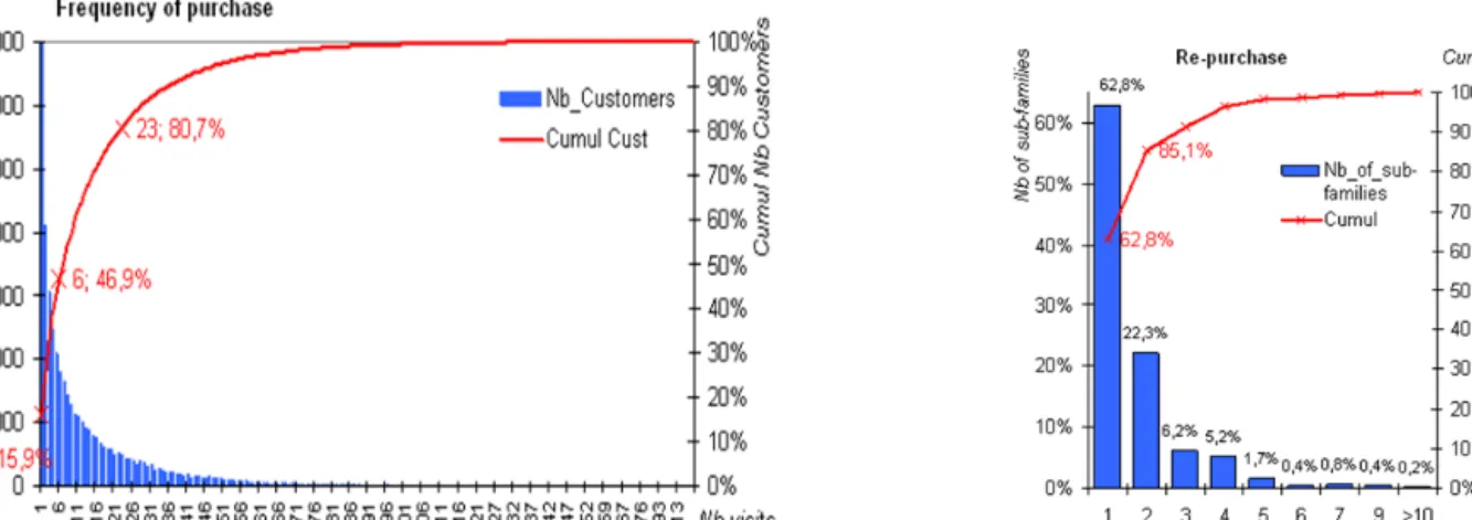
Figure 2: Frequency of purchase (left) and Re-purchase (right)

purchases the complete set of products he’ll need: they can suggest missing products and show him the products in the relevant department. BAO thus launched a project to have recommendations produced in real-time for the salesperson to use in his discussion with the customer: salespeople are equipped with a PDA, which can read the loyalty card and the products bar-codes and to which the recommendations are to be sent. This scenario is represented in Figure 1. Less experienced vendors would certainly benefit more from the recommendation application, but even seasoned vendors have expressed their interest for it, saying that this could work for them as a check list of all the products needed. As can be seen, the setting for our recommender system is rather original, since most systems in the literature have been developed for on-line retailers.

The deployment scenario chosen by BAO was to first de-sign and evaluate a recommender system on data from its major store; then to test it on the field in that store and finally deploy it throughout all the 27 stores. This paper reports on the first phase, where various techniques had to be evaluated for designing the best system, while phase 2 is presently ongoing.

The dataset we used contains all purchase history from loyal customers at BAO’s major store from 2005 to 2008. As we shall see later, data from 2005 to 2007 were used for training and data for 2008 for testing. It corresponds to 43,779 customers and 3,425,048 transactions for training (from 2005 to 2007), and 30,784 customers (of which 6,923 are new customers) and 1,140,510 transactions for testing. The items we consider are not individual products but rather groups of products or sub-families, because BAO decided that recommendations should be made at this level of their product hierarchy. An example of sub-family is “pipe”, while individual products are pipes of varying length, color, . . .

This will leave more space for the salesperson’s expertise and should be easier to use in the intended context. We selected only the sub-families which were sold every year of the training data, and obtained 484 sub-families.

Figure 2 shows various characteristics of the 2005-2007 data: a RFM analysis showed that 15.9% customers visited only once (and 80.7% 23 times at most) and 15% sub-families were bought at least 3 times by the same customer. Since we are working at the sub-families level, this situation should be expected in our case, as well as in a DVD retail industry

for example, where customers typically buy various times at the genre – sub-family – level, yet each product once at most at the product level. This implies in particular that we need to potentially recommend an item (i.e. a sub-family) which has already been purchased by the same user.

As usual in retail contexts, data show a marked Long Tail effect [4]: 30% of the 484 sub-families (vigintiles 1 to 6) rep-resent 81.8% of total sales (these are theHead sub-families); while the last 11 vigintiles (10 to 20) represent 55% of the sub-families and account for only 8.1% of sales (theTail). Obviously, data are very sparse in the Tail and it will thus be harder to produce relevant recommendations in the Tail than in the Head. Being able to accurately recommend Mid-dle or Tail items can however be an interesting property of a recommender system since it may correspond to more un-expected suggestions. We will see in our experiments that some algorithms essentially predict Head items, while some others are able to find some relevant Tail products.

Figure 3: Total number of sales for each vigintile (5%) of sub-families.

3. GENERAL EXPERIMENTAL PROTOCOL

AND EVALUATION METRICS

We now present our experimental protocol. In our setup, a CF algorithm can be seen as a black box, which takes as input apurchase matrix, and outputs a predictor. The pur-chase matrix summarizes the training data (the transactions from 2005 to 2007 in our case) as described in Subsection

(4)

3.1. A predictor can be seen as a black box as well, which takes as input a customer’s purchase history and outputs a sorted list of the 484 items. The quality of the sorted list is measured by comparing the first recommended items with items bought by the same customer in a near future. Our goal is to measure the ability of the system to perform rel-evant recommendations when the user is in the shop. In many cases, a customer needs a product for a particular short-term project, so our evaluation has to measure the quality of the predictions in the short-term. To that end, we decompose our test data (i.e. the 2008 purchase data) into several smaller sets, each of which is based on a specific daydof 2008, and we try to predict the items purchased by a customer within 2 weeks after that day, using the customer’s purchase history known atd. The construction of these test sets is detailed in Subsection 3.2, and the evaluation metrics are defined in Subsection 3.3. How we train and test each algorithm is described later in the next Section.

3.1 Purchase Matrix

The training stage of the algorithms we evaluate takes as input apurchase matrix, where each column corresponds to an item, and each row represents apurchase session. A (pur-chase) sessionshould be understood as “the set of purchases of a given customer over a period of time”. In standard col-laborative filtering approaches (see e.g. [2]) and in Section 5 of this paper, a row of the purchase matrix represents the total purchase history of a specific customer. In that case, a purchase session is defined as “all known purchases of a cus-tomer” without limitation in time, but we will also consider purchase sessions defined on smaller periods of time in Sec-tion 6. In all cases, a purchase matrix, denotedP, contains only Boolean values (0 or 1), where a 1 in the (i, k)th entry means that itemkhas been bought at least once in thei-th session (0 means the opposite). In the following,R (resp.

C) will denote the number of rows (resp. columns) ofP.

3.2 Test data

As we intend to predict the future purchases of customers in the short term, we evaluate the various algorithms with a sliding window approach: for every day d of the testing period and every customer who made a purchase on that day, we predict his purchases for the next 14 days (includ-ing the reference day d, to predict the final purchases of the customer that day), based on his purchase history (i.e. the products bought strictly before the reference day). The window length of 14 days has been chosen by business con-straints. It is motivated by the observation that most sales arecomplete within 14 days after the first purchase of this sale. In the end, there are 298 reference days and thus 298 test sets: each day of 2008 is a reference day except Sundays, holidays (when the shop is closed), and the last 13 days of 2008 (the purchases for the next 14 days are not available). After creating the test sets, we filter some customers out of each set. For each test set, we discard all customers who did not make any purchase within 14 days before the corre-sponding reference day (excluded).4 _{This selection is once}

again motivated by the fact that sales are complete within 14 days, and will allow us to compare various experimental settings on the same set of customers.

4_{Note that customers not present on the reference day are}

not included in the test set either, since we can only make recommendations to customers present in the store.

3.3 Evaluation Metrics

The recommendation algorithms output a sorted list of items given the purchase history of a customer at a given date. Following [9, 8], we use precision, recall and F1-score to evaluate the quality of a recommendation list. These met-rics are then averaged over customers and time to provide a final performance value. In our approach, we have a set of customers for each reference day, together with a target set of products for each customer (recall that the target set con-tains the customer’s purchases for the next 14 days, and thus depends on the reference day). For a given customeruand a given reference dayd, the precision, recall and F1-score of theN first recommended items are respectively defined as:

• precu,d@N=

card Ru,d@N∩Tu,d

N ,

• recu,d@N=

card Ru,d@N∩Tu,d

card Tu,d

where givenuandd,Tu,dis the target set andRu,d@N

the set of top-N recommended items.

• F1u,d@N=

2.recu,[email protected],d@N

rec_u,d@N+prec_u,d@N.

The value of the cutoffN is chosen by business constraints. In our case, only 5 recommendations will be presented, so these measures are of greatest interest withN= 5.

To compute the final performance values, we first average over users for each reference day. The precision obtained for the reference daydis given by:

precd@N =

X

u:test user for dayd

precu,d@N

nb of test users for dayd.

Similar formulas are used to obtainrecd@N(resp.F1d@N),

the recall (resp. F1-score) for the reference day d. The final performances are then computed by averaging over all possible reference days:

perf@N=

X

d:reference day perfd@N

nb of reference days forperf∈ {prec, rec, F1}.

4. ALGORITHMS EVALUATED

We have selected a number of algorithms from the three main families of collaborative filtering approaches: memory-based, model-based and association rule learning. For the memory-based technique, we consider the item-based ap-proach [16], in which the bulk of the computation is done offline. For model-based approaches, we selected two state-of-the-art matrix factorization methods, Singular Value De-composition [23] and Non-Negative Matrix Factorization [27]. For association rule learning, we build the bigram matrix [22] (i.e. all rules of the form item i⇒item j). The choices of the algorithms are arbitrary, we only intended to have rep-resentative algorithms for each of the main CF approaches.

4.1 Training the Algorithms

Item-Based Collaborative Filtering.

The item-based approach computes, on the training pur-chase data, a similarity matrix between products. Following Linden et al. [16], we compute the similarity between the

(5)

two productsk and`using the cosine between their corre-sponding columns of the purchase matrix:

sim k, `= P T •kP•` p PT •kP•k p PT •`P•`

whereP•kis thek-th column ofP, andXTis the transpose

of matrix X. The output of the training process is then the similarity matrix between productsS, where the (k, `)th entry ofSis equal to sim k, `

.

Matrix Factorization Methods.

Matrix factorization methods have shown great perfor-mance for ratings prediction [14, 26]. To apply these meth-ods on purchase data, we use the AMAN (all missing as negative) reduction [20]. In this setup, matrix factorizations approximate the purchase matrixP∈RR×Cby a matrix of

smaller rankr(rrank P

). The approximation can be written as the productU?_V? _{of two matrices} _U? _∈

RR×r

andV? ∈Rr×C. We first evaluate the factorization which

gives the best rank-rapproximation ofPin the sense of the Frobenius norm which can be found using_svd[23]:

U?,V?= arg min U∈RR×r,V∈Rr×C kP−UVk2_F (1) wherekXk_F =qP i,jx 2

i,j is the Frobenius norm ofXand

xi,j the (i, j)thentry ofX. We also tried to weight missing

entries as in [20], but it did not improve performances, so these results are not presented in our experiments.

We also evaluate non-negative matrix factorization (nnmf) which was shown to have good performances in CF [27].

nnmffinds an approximation of the purchase matrix with

factors constrained to only have non-negative elements:

U?,V?= arg min

U∈RR×r+ ,V∈R

r×C

+

kP−UVk2F . (2)

For any matrix factorization method (svd, nnmf, or any other), the rightmost matrixV? can be seen as an embed-ding matrix, which projects every productk in_Rr _(or

Rr+

for_nnmf). Thus, the k-th column of V?_,_V?

•k, can be

in-terpreted as a representation of productkin the embedding space. On the other hand,U?expresses the rows of the pur-chase matrix as a linear combination of lines ofV?_{, and is}

thus representative of the training data only. Consequently, after obtaining a factorization of the training purchase ma-trixPof the form U?_V?_,_U? _{is not stored. The only}

pa-rameter resulting from training is matrixV?.

Association Rules.

We also evaluate association rule learning for CF [22, 11]. We first consider bigram rules, where training simply con-sists in computing the following matrix on the purchase data:

B= [bk,`]k=1..C `=1..C with bk,`= PT•kP•` kP•kk1 , kXk₁= C X k=1 |xk| (3)

bk,` is thus the confidence of rulek⇒`(i.e. item k is

pur-chasedimpliesitem`is purchased within the same session). Special care needs to be taken for diagonal elementsbk,k:

they are all equal to 1 in (3), which does not reflect the real probability that itemk was bought twice at different times within the same session. Although the true confidence of the rulek⇒k cannot be computed from the purchase matrix,

we compute it from the initial transactional data as follows:

bk,k=

nb sessions wherekwas bought at least twice nb of sessions wherek was bought . Since bigram rules consider at most two items without any consideration of their support, we tried a more refined ver-sion of associations rules (called alpha-rules in the paper) based on the concepts of alpha Galois lattice [25] and fre-quent closed itemsets [21]. alpha-rule learning aims at scal-ing up the rule minscal-ing usscal-ing domain knowledge provided as a segmentation of purchase sessions: the algorithm only finds closed itemsets and rules satisfied by at leastα% sessions of a given segment (the parameterαcontrols the complexity of the method). This method is only applicable when having a typology of purchase sessions (which will be built in Section 6), so we only present its results after Section 6.

4.2 Applying the Algorithms

At apply time, an algorithm is given a customer’s purchase history (which contains all past purchases of a customer or only the most recent ones), and is required to provide a list ofN recommendations for this user (N = 5 in our case). A purchase history is represented by a Boolean column vector

H ∈ {0,1}1×C

, where 1 at the kth line means that item

k has been bought by the customer at least once over the period considered for building the history. H contains the purchases of a single customer, so the prediction processes described below are applied to each customer of a test set. Note that our prediction processes can be applied to any customer, even if he was not seen during training.

Item-Based CF Prediction.

The recommendation list for item-based collaborative fil-tering is created as follows:

1. For each itemk inH(i.e. ks.t. hk= 1), select theS

items which are the most similar tok using the simi-larity matrixScomputed during training. We obtain

kHk₁lists of items with similarity scores for each item in each list. In our experiments we use S = 20 as it tended to give the best results.

2. Merge the lists: concatenate the lists, and sort the items by decreasing associated score. If an item is in several lists, assign it its maximum score.

Prediction with Matrix Methods.

The inference procedure corresponds to the setting ofstrong generalization [18]. This setting allows us to make predic-tion for new customers or to take into account the updates (if any) of the customer’s purchase history. Given the embed-ding matrixV? learnt on the training data, we compute a parameter vectorW?such thatW?TV?approximates best the user’s purchase history H. Depending on the method,

W?is defined as follows: • svd:W?=arg min W∈_Rr W T V?−H 2 FwithV ? given by (1), • nnmf:W?=arg min W∈_Rr + W T V?−H 2 FwithV ? given by (2).

Both are convex quadratic problems which can be solved very efficiently at apply time. Once the parameter vector

(6)

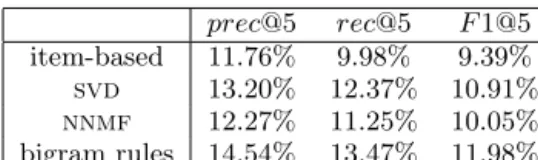
Table 1: Test results for theComplete History (left) and the 2 Weeks History (right) apply settings, when the algorithms are trained on theuser×item purchase matrix. Relative differences of more than 5% on any metric and between any two algorithms are significant.

prec@5 rec@5 F1@5 item-based 6.87% 6.10% 5.62% svd 13.22% 12.39% 10.92% nnmf 11.28% 9.35% 8.85% bigram rules 10.88% 9.33% 8.64% prec@5 rec@5 F1@5 item-based 11.76% 9.98% 9.39% svd 13.20% 12.37% 10.91% nnmf 12.27% 11.25% 10.05% bigram rules 14.54% 13.47% 11.98%

W? is computed, all items are sorted by decreasing scores (the predicted score for itemkisW?TV?•k in both cases).

Prediction with Association Rules.

For bigram rules, we follow [22]: itemskare sorted by the maximum confidence of the rules `⇒k supported by the user history (i.e. `is such thath`= 1). The prediction with

alpha-rules is similar.

5. A STANDARD APPROACH

We first evaluate what we refer to as the standard ap-proach. This corresponds to the case where each row of the training purchase matrix contains all known purchases of all training customers, called the user×item matrix. In that case, the training purchase matrix has a sparsity coefficient of 5.7%. After training each algorithm according to Section 4.1, we evaluate 2 differentapply settings:

Complete History In theComplete Historyapply setting, the prediction algorithms (described in Section 4.2) re-ceive as input a purchase vector which containsall past purchases of this customer without limitation in time. Thus, for a given reference day and a given customer, the prediction will be based on all of this customer’s purchases made strictly before the reference day.

2 Weeks History In the 2 Weeks History apply setting, the prediction algorithms receive as input a purchase vector containing only the customer’s purchases made in the last 14 days before the reference day (excluded). We remind to the reader that(1)the training procedure of the algorithms is the same for both apply settings, (2)

thanks to the filter applied to the test sets (Subsection 3.2), the algorithms are evaluated on exactly the same customers and target sets, and finally(3)the reported performance for both apply settings are computed on the test data following the protocol described in Subsection 3.2.

The test performances in terms of prec@5, rec@5 and

F1@5 for the various algorithms and the two apply settings are shown in Table 1. The rank of matrix factorization is chosen based onF1@5 (r= 20 for both methods).

The results first show that bigram association rules in the 2 weeks history apply setting obtain the best results, with relative performance gains between 8% and 10% on all met-rics. However, we have to notice that in theComplete His-toryapply setting, factorization methods obtain the best re-sults. Thus the relative performances of the methods change when taking recency into account. It implies that no general conclusion can be drawn from the relative performances of each algorithm in a specific application scenario, and that testing each method for each scenario is mandatory.

When comparing the two apply settings, we see that con-sidering only the most recent purchases has a positive impact

on all performances, except for the_svdon which the differ-ence is not significant. This suggests that only purchases made within a short period of time are strongly correlated, so that the recency of the purchase may be a critical fac-tor for the recommendation. Similar observations have al-ready been reported (see e.g. [14, 15]) on other datasets where users’ tastes evolve with time. Even though the rea-son might be different in our case (see Section 6), our results give additional evidence that the recency of user feedback is an important factor in CF. In particular, it appears to be crucial for item-based CF and association rules. This is due to the aggregation scheme we chose (the max of the items similarities or rules’ confidences), which is not robust to this noise. We carried out additional experiments (not reported here) where we used thesum of the rules’ confidence (as in [11]) instead of the max for association rules. The algorithm becomes then more robust, with less than 15% relative dif-ference inprec@5 between the two settings (instead of about 30% with the max as reported in Table 1). The same be-havior was observed for item-based CF. The algorithms do not perform better though, because adding low confidences eventually leads to overcome the confidence of relevant rules. In terms of absolute performance values, the best preci-sion at 5 is lower than 15%. Acceptance of the system on the field will be hard: when the salesperson recommends 5 products to his customer, the latter will buy less than once on average. Sales staff will soon stop proposing recommen-dations to avoid losing the customers’ confidence. We need better performances, at least 20% of precision to ensure that at least one product is bought by the customer on average.

6. A BUSINESS-ORIENTED APPROACH

The business of BAO is to sell products to customers for home improvement. This customers’ activity has its speci-ficities, one of which was highlighted in the previous sec-tion: customers have a purchasing behavior which varies a lot in time. At some periods, they only buy little, and only standard products (electric bulbs, nails,. . .); while at other periods, they launch aprojectsuch as refurbishing the bathroom or putting a new roof. Projects requires more spending, more - very specific - products and this over a rel-atively short period. In this section, we try and exploit this behavior to focus on such specific activity, because it should allow us to narrow the potential choice of relevant products and thus recommend products at a given time depending on what the customer is doing at that time. From a business perspective, the recommender system should be most useful if it can help getting a complete sale for customers running a project, i.e. a sale where all the products necessary for that project are actually purchased.

We show how to detect projects periods in customers’ pur-chase histories and automatically categorize them in

(7)

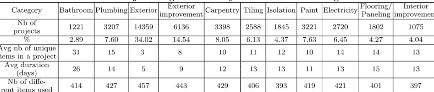
Subsec-Table 2: Project categories found by k-means on the training data.

Category Bathroom Plumbing Exterior Exterior Carpentry Tiling Isolation Paint ElectricityFlooring/ Interior

improvement Paneling improvement

Nb of 1221 3207 14359 6136 3398 2588 1845 3221 2720 1802 1075 projects % 2.89 7.60 34.02 14.54 8.05 6.13 4.37 7.63 6.45 4.27 4.04 Avg nb of unique 31 15 3 8 10 11 12 10 14 14 13 items in a project Avg duration ₂₆ ₁₄ ₅ ₉ ₁₂ ₁₃ ₁₃ ₁₁ ₁₃ ₁₅ ₁₃ (days) Nb of diffe-414 427 457 443 429 406 393 419 421 401 397

rent items used

Table 3: Test results for theComplete History (left) and the2Weeks History (right) apply settings when the algorithms are trained on the project×item matrix. A relative difference of more than 5% in any metric is always statistically significant.

prec@5 rec@5 F1@5 item-based 5.41% 4.91% 4.43% svd 12.85% 11.80% 10.53% nnmf 11.08% 9.43% 8.81% bigram rules 9.52% 8.71% 7.71% alpha-rules 14.19% 6.65% 8.53% prec@5 rec@5 F1@5 item-based 10.85% 9.57% 8.77% svd 12.90% 11.83% 10.56% nnmf 12.48% 11.39% 10.20% bigram rules 15.84% 16.42% 13.67% alpha-rules 16.10% 7.57% 9.70%

tion 6.1. We then study two strategies to integrate projects and their categories in the recommendation process.

6.1 Project Definition and Categorization

The domain experts at BAO observed that past customers’ projects can be extracted from their purchase history by identifying high purchase activity periods, defined as peri-ods where a given customer spends at least 200e over a duration of 14 days. BAO has specialized salespeople for customers running very large projects (i.e. building a house) and wants to exclude these from the perimeter of the rec-ommender system. We thus extracted from the 2005-2007 dataset all projects by isolating high-purchase activity pe-riods of the customers, discarding projects that last more than 50 days or with a total expense greater than 2,000e. We then merged projects separated by less than a week and eliminated all no-purchase days at the end of the 42,202 identified projects to calculate the real project duration. Fi-nally, projects account for about 1/3 of all the transactions, and 50% of the customers are involved in at least one project. We built a typology of projects using k-means5supervised by the number of items used in the project. We found a typology of 11 segments which were analyzed by business-owners who found a description as meaningful project cate-gories. These categories are descriptive of the context of a purchase, such as plumbing or painting. The segments are summarized in Table 2. The two larger categories, account for 34% and 14.5% of all projects. All other categories (ex-cept for the smallest one) contain between 4% and 8% of the projects. Most categories contain projects which involve, on average, about 10 different unique items (with possibility of re-purchase), but more than 400 items are used in at least one project of each category (thus, more than 80% of the total number of items). Thus, even if the project categories contain more homogeneous sets of purchases, recommenda-tion must cover most of the catalog.

5

We used KXEN K2S segmentation module (KXEN AF v5.0.5,www.kxen.com.)

6.2 Training on Projects Only

We saw in Section 5 that considering only a short-term purchase history at prediction time increases the recommen-dation accuracy. Together with the analysis of projects, these results suggest that only short-term correlations tween two purchases are relevant, long-term correlations be-ing most probably accidental. We propose to integrate this additional knowledge into the training process, by learning on a modified purchase matrix which contains one row for each project detected in the period 2005-2007. We obtain a

project×item purchase matrix of size 42,202×484. It has a higher sparsity than the user×item matrix (2.3% non-zero entries instead of 5.7%) but is also less noisy. Remember that the purchase matrix is only used to compute item/item similarities for item-based CF, the item projection matrix for factorization methods, and the confidence of the associ-ation rules. Thus, the models trained on this new purchase matrix are applied the same way as in Section 5. alpha-rules are trained on theproject×item matrix like the other algo-rithms, but unlike them uses the categorization of projects for a faster exploration of the search space.

Recommendation performance.

The performances of the models in both the Complete History and the 2 Weeks History apply settings are shown in Table 3. The optimal rank for _svd and _nnmf is still

r = 20. alpha-rules are withα= 10% and a minimal sup-port of 1%. The differences in performances between the two apply settings are similar to those of the previous sec-tion. In the Complete History apply setting, the models perform worse than in the previous section, which is natural since they are trained on purchase sessions that span over shorter periods of times. In the 2 Weeks Historyapply set-ting, the results are similar to the previous results, except for the bigram rules which obtain significantly better per-formances, with a greater improvement of the recall (more than 20% relative increase). Thus, the benefit of training on the project×item matrix mostly concerns customers for which few items had to be predicted. alpha-rules obtain slightly better performances in terms of precision, but their

(8)

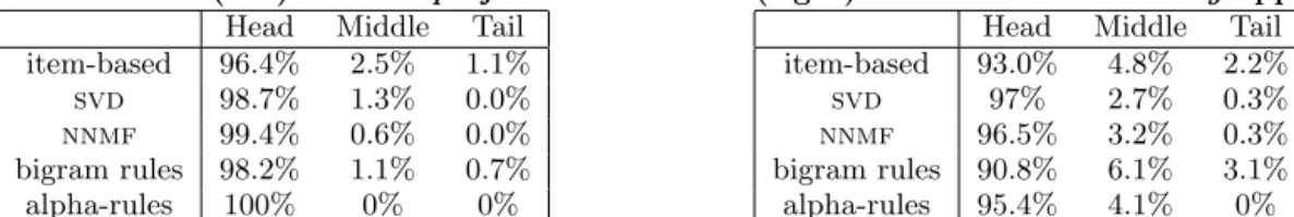
Table 4: Proportion of recommended and purchased items in the Head, the Middle and the Tail when training on theuser×item matrix (left) and the project×item matrix (right) in the2 Weeks History apply setting.

Head Middle Tail item-based 96.4% 2.5% 1.1%

svd 98.7% 1.3% 0.0% nnmf 99.4% 0.6% 0.0%

bigram rules 98.2% 1.1% 0.7% alpha-rules 100% 0% 0%

Head Middle Tail item-based 93.0% 4.8% 2.2%

svd 97% 2.7% 0.3%

nnmf 96.5% 3.2% 0.3%

bigram rules 90.8% 6.1% 3.1% alpha-rules 95.4% 4.1% 0%

Table 5: Test results of non-contextual (left) and contextual (right) recommendations on the subset of users running a project on the reference day, in the2Weeks Historyapply setting. The non-contextualproject×item

model is trained and applied as in Section 6.2. The contextual model is described in Section 6.3. prec@5 rec@5 F1@5 item-based 15.08% 9.73% 10.53% svd 21.17% 11.21% 13.56% nnmf 20.64% 10.97% 13.23% bigram rules 24.15% 13.46% 15.88% alpha-rules 25.70% 7.31% 9.40% prec@5 rec@5 F1@5 item-based 20.61% 12.83% 14.17% svd 24.30% 12.17% 15.22% nnmf 26.26% 13.38% 16.57% bigram rules 32.46% 17.69% 21.15% alpha-rules 27.57% 12.81% 16.59%

recall andF1 is rather low. This is essentially due to the high setting of the minimal support, but decreasing it leads to very high complexity.

Recommended items.

The models trained on theproject×item matrix produce slightly different recommendations than those trained on the

user×item matrix. Table 4 compares these models in the 2

Weeks Historyapply setting. It shows, among the items that were recommended and actually purchased by the customer, the percentage of items belong to the Head (i.e. best-sellers), the Middle or the Tail. The Tail, which contains 55% of the items but account for only 8.1% of the sales (see Section 2) contains items that are very difficult to recommend at the right moment. Indeed, the models of the previous sec-tion are only able to make accurate recommendasec-tions in the Head (more than 95% of the correct recommendations for all models). The reason is that complete customers’ purchase histories contain mostly Head items, so that Middle and Tail items are filtered out as noise by the algorithms. A larger part of the correct recommendations lies in the Middle or Tail when training on the project×item where short-term correlations between Middle or Tail products can be dis-covered. In particular, more than 9% of the bigram rules’ correct recommendation are now Middle or Tail items.

6.3 Contextual Recommendation

The analysis of projects shows that a typology of more ho-mogeneous purchase patterns can be found, and that these categories, such as “interior” or “exterior” improvement, have a clear interpretation in terms of contextual variables that describe the intent of the purchase. Following the multidi-mensional model of [2], we propose to evaluate the gain in predictive performance if oneknew this context at predic-tion time. This is particularly relevant for our applicapredic-tion, since we have very broad context descriptions: the context might be simply inferred by the salesperson during a nor-mal dialogue with the customer; even asking for it has not be seen as too intrusive by professionals.

In the simplest form of the multidimensional model, given the context in which a recommendation is made, the predic-tion is based solely on past purchases made within the same context. In our case, this is implemented as follows:

• At training time, we train 11 models, one for each

category of projects (or, equivalently, we train one model for each possible context). Each of these models is trained on a specificproject×item purchase matrix containing one row for each project of 2005-2007 of the corresponding category.

• At apply time, we assume that we know the category of the current customer’s project (i.e. we know the context of the purchase). On the test data, this is sim-ulated by filtering out all transactions of 2008 which do not belong to a project, and by assigning to each re-maining transaction the project category it belongs to. Then, for each user and each reference day, we apply the model which corresponds to the project category. As we do not evaluate on exactly the same set of transac-tions as in Sectransac-tions 5 and 6.2, we also provide, on this set of transactions, the results obtained by the non-contextual model of Sections 6.2 as a baseline. Note that it is exactly the same model and predictions as in Section 6.2, but we consider now only the test users and transactions that be-long to a high purchase activity at the reference day. Due to lack of space, we only report the results of the models in the 2Weeks Historyapply setting6. These performances are shown in Table 5. Factorization methods use a rankr= 5.

The non-contextual models, on this subset of transac-tions, have higher precision and lower recall than in general (compare Table 3 (right) and Table 5 (left)), because peo-ple running projects buy more products, artificially inflating

prec@5 and decreasing rec@5. The effect of contextualiza-tion, however, is critical: item-based CF,_nnmfand bigram rules show a relative increase of at least 30% in all perfor-mance values. The effect is less dramatic for svd (which tends to be the most constant model on our data) and for alpha-rules which already used the typology in the explo-ration of the rules. More interestingly, bigram rules have a precision of 32%. Thus, on average, between 1 and 2 recom-mended products are actually bought by the customer. We also note that despite their simplicity, bigram rules perform significantly better than other methods on all measures.

Our results, in line with recent works [5, 19], provide addi-tional evidence of the importance of the context of a

recom-6_{The performances of the algorithms in the}_Complete His-tory apply setting, and the results of the models trained as in Section 5, are consistently worse.

(9)

mendation. Such performances are acceptable in a dialogue with a customer. Even though this only affects a part of our test data (about 1/3 of transactions), these are the transac-tions that involve the greater number of items, and thus for which the recommender system should be of greater interest. When looking at which items are recommended and pur-chased, we see that the better performances obtained by the contextual models are due to more accurate recommenda-tions of best-sellers: for all algorithms, at least 95% of the correct recommendations involve Head items.

7. CONCLUSION

We presented a systematic comparison of various collab-orative filtering systems on a real-life purchase dataset. We showed that recommender systems can be developed on pur-chase rather thanrating data, and that, in such cases, al-gorithms comparison is different from the standard rating case. In particular, on our data, the simplest algorithm based on bigram association rules obtained the best perfor-mances. We believe that such case-studies are necessary to better understand the specificities of purchase datasets and the factors that impact recommender systems for retailers.

Our results show that factors such as purchase recency and context-awareness may be at least as important as the choice or the design of a well-performing algorithm. They also show that the relative performances of the algorithms vary depending on the setting to which they are applied, so that all algorithms have to be tested at all stages of the development of the recommender system.

Acknowledgements

The authors thank A. Bordes, D. Buffoni, S. Canu, A. Spen-gler and G. Wisniewski for fruitful discussions. This work was partially funded by the ANR (CADI project).

8. REFERENCES

[1] G. Adomavicius, R. Sankaranarayanan, S. Sen, and A. Tuzhilin. Incorporating Contextual Information in Recommender Systems Using a Multidimensional Approach.Trans. on Inf. Sys., 23(1):103–145, 2005. [2] G. Adomavicius and A. Tuzhilin. Towards the Next

Generation of Recommender Systems: A Survey of the State-of-the-Art and Possible Extensions.IEEE Trans. on Knowledge and Data Eng., 17(6):734–749, 2005. [3] G. Adomavicius and A. Tuzhilin. Context-aware

Recommender Systems. InProc. of the 2008 ACM Conf. on Rec. Sys., pages 335–336, 2008.

[4] C. Anderson.The Long Tail: Why the Future of Business Is Selling Less of More. Hyperion, 2006. [5] L. Baltrunas. Exploiting Contextual Information in

Recommender Systems. InProc of the 2008 ACM Conf. on Rec. Sys., pages 295–298, 2008.

[6] R. Bell, Y. Koren, and C. Volinsky. Chasing

1,000,000$: How We Won the Netflix Prize.ASA Stat. and Computing Graphics Newsletter, 18(2), 2007. [7] Y. Ding, X. Li, and M. E. Orlowska. Recency-based

Collaborative Filtering. InProc. of the 17th Australasian Database Conf., pages 99–107, 2006. [8] A. Gunawardana and G. Shani. A survey of accuracy

evaluation metrics of recommendation tasks.J. Mach. Learn. Res., 10:2935–2962, 2009.

[9] J. L. Herlocker, J. A. Konstan, L. G. Terveen, and J. T. Riedl. Evaluating Collaborative Filtering Recommender Systems.ACM Trans. on Inf. Sys., 22(1):5–53, 2004.

[10] Y. Hu, Y. Koren, and C. Volinsky. Collaborative Filtering for Implicit Feedback Datasets. InProc. of ICDM, pages 263–272, 2008.

[11] C. Kim and J. Kim. A Recommendation Algorithm Using Multi-Level Association Rules. InProc. of the 2003 IEEE/WIC Intl. Conf. on Web Intel., 2003. [12] Y. Koren. Factorization Meets the Neighborhood: a

Multifaceted Collaborative Filtering Model. InProc. of SIGKDD, pages 426–434, 2008.

[13] Y. Koren. Collaborative filtering with temporal dynamics.Commun. ACM, 53(4):89–97, 2010. [14] Y. Koren, R. Bell, and C. Volinsky. Matrix

Factorization Techniques for Recommender Systems.

Computer, 42(8):30–37, 2009.

[15] T. Q. Lee, Y. Park, and Y.-T. Park. An Empirical Study on Effectiveness of Temporal Information as Implicit Ratings.Expert Syst. Appl., 36(2):1315–1321, 2009.

[16] G. Linden, B. Smith, and J. York. Amazon.com Recommendations: Item-to-Item Collaborative Filtering.IEEE Internet Computing, 7:76–80, 2003. [17] J. Liu, M. Z. Q. Chen, J. Chen, F. Deng, H. Zhang, Z. Zhang, and T. Zhou. Recent Advances in Personal Recommender Systems.J. of Inf. and Sys. Science, 5(2):230–247, 2009.

[18] B. Marlin. Collaborative Filtering: A Machine Learning Perspective. Master’s thesis, University of Toronto, 2004.

[19] C. Palmisano, A. Tuzhilin, and M. Gorgoglione. Using Context to Improve Predictive Modeling of Customers in Personalization Applications.IEEE Trans. on Knowl. and Data Eng., 20(11):1535–1549, 2008. [20] R. Pan and M. Scholz. Mind the Gaps: Weighting the

Unknown in Large-Scale One-Class Collaborative Filtering. InProc of SIGKDD, pages 667–676, 2009. [21] N. Pasquier, R. Taouil, Y. Bastide, G. Stumme, and L. Lakhal. Generating a condensed representation for association rules.J. Intell. Inf. Syst., 24(1):29–60, 2005.

[22] B. Sarwar, G. Karypis, J. Konstan, and J. Riedl. Analysis of Recommendation Algorithms for e-Commerce. InProc. of the 2nd ACM Conf. on Electronic Commerce, pages 158–167, 2000. [23] N. Srebro and T. Jaakkola. Weighted Low-Rank

Approximations. InProc. of the 20th Intl. Conf. on Mach. Learn., pages 720–727, 2003.

[24] X. Su and T. M. Khoshgoftaar. A survey of Collaborative Filtering Techniques.Adv. in Artif. Intell., 2009:2–2, 2009.

[25] V. Ventos and H. Soldano. Alpha galois lattices: An overview. InICFCA, pages 299–314, 2005.

[26] M. Weimer, A. Karatzoglou, and A. J. Smola. Improving maximum margin matrix factorization.

Machine Learning, 72(3):263–276, 2008.

[27] S. Zhang, W. Wang, J. Ford, and F. Makedon. Learn-ing from incomplete ratLearn-ings usLearn-ing non-negative matrix factorization. InProc. of SDM, pages 549–553, 1996.