Microaneurysm Detection using Deep Learning and
Interleaved Freezing
Piotr Chudzik
a, Somshubra Majumdar
b, Francesco Caliva
a, Bashir Al-Diri
a, and Andrew
Hunter
aa
School of Computer Science, University of Lincoln, Lincoln, United Kingdom
bDepartment of Computer Science, University of Illinois, IL 60607, Chicago, USA.
ABSTRACT
Diabetes affects one in eleven adults. Diabetic retinopathy is a microvascular complication of diabetes and the leading cause of blindness in the working-age population. Microaneurysms are the earliest clinical signs of diabetic retinopathy. This paper proposes an automatic method for detecting microaneurysms in fundus photographies. A novel patch-based fully convolutional neural network for detection of microaneurysms is proposed. Compared to other methods that require five processing stages, it requires only two. Furthermore, a novel network fine-tuning scheme called Interleaved Freezing is presented. This procedure significantly reduces the amount of time needed to re-train a network and produces competitive results. The proposed method was evaluated using publicly available and widely used datasets: E-Ophtha and ROC. It outperforms the state-of-the-art methods in terms of free-response receiver operatic characteristic (FROC) metric. Simplicity, performance, efficiency and robustness of the proposed method demonstrates its suitability for diabetic retinopathy screening applications.
Keywords: Deep Learning, Fundus Photography, Convolutional Neural Networks, Diabetic Retinopathy. Mi-croaneurysm Detection
1. INTRODUCTION
Diabetic retinopathy (DR) is a microvascular complication of diabetes and the leading cause of vision loss in the working-age population.1 DR screening is manually performed by ophthalmologists and trained graders through a visual inspection of fundus photographies (FP). Unfortunately, the grading process is time-consuming, tedious, and error-prone with high inter-observer variability. Due to the rising number of DR patients worldwide (expected 640 millions by 20402) and their location (75% live in underdeveloped areas3) the development of automatic DR screening approaches is of utmost importance.
Microaneurysms (MAs) are spherical swellings of the capillaries caused by weakening of the vascular walls that appear as small round red dots. MA detection is a challenging task even for the human eye due to many factors including limited resolution, reflections, uneven image illumination and media opacity. The boundaries of MAs are not always well-defined and local contrast to the background is low, even in high-resolution images. Moreover, MAs may be confounded with visually similar anatomical structures such as haemorrhages, junctions in thin vessels, disconnected vessel segments, dark patches on vessels, background pigmentation patches and dust particles on the camera lense. They are the earliest clinical signs of DR which continue to be present as the disease progresses. As such, the automated detection of MAs can drastically reduce the screening workload.
The main contributions of this paper are as follows. First, we propose an automatic MA detection method that requires only two stages of analyses. Second, we present a novel FCNN with dedicated architecture for MA
Further author information: (Send correspondence to P.C.) P.C.: E-mail: [email protected],
S.M.: E-mail: [email protected], F.C.: E-mail: [email protected], B.A.: E-mail: [email protected], A.H.: E-mail: [email protected].
detection that does not require hand-crafted features. Third, we propose a novel fine-tuning technique called Interleaved Freezing, that significantly reduces the amount of training time and number of required experiments. This paper is organized as follows. The related work is described in Section II. Section III describes the datasets and performance metrics used for experiments. The proposed method is described in Section IV. Section V presents evaluation results and comparison with existing approaches. Finally, in Section VI discussion and conclusions are given.
2. RELATED WORK
The vast majority of MA detection methods consists of five consecutive processing stages: 1) Preprocessing, 2) MA candidate extraction, 3) Vessels removal, 4) Candidate feature extraction, and 5) Classification. Baudoin
et al.4 introduced the first MA detection algorithm applied to fluorescein angiogram images. They employed a mathematical morphology based approach to remove vessels and applied a top-hat transformation with linear structuring elements to detect MAs. Several methods were built on this approach,5 however, since intravenous use of fluorescein can cause death in 1 in 222 000 cases,6 such methods are not suited for screening purposes. Walter et al.7 also used a top-hat based method and automated thresholding to extract MA candidates. They extracted 15 features and applied kernel density estimation with variable bandwith for MA classification. In general, morphology-based approaches are sensitive to changes in size and shape of structuring elements which result in significant variations in MAs detection results. Zhang et al.8 proposed a method based on dynamic thresholding and correlation coefficients of a multi-scale Gaussian template. They used 31 manually designed features based on intensity, shape and response of a Gaussian filter. Veigaet al.9 presented an algorithm using Law texture features. Support Vector Machines (SVM) were used in a cascading manner: first SVM was used to extract MA candidates whereas the second SVM performed final MA classification. Javidiet al.5 proposed a technique which used 2D Morlet wavelet to find MA candidates. At the next stage, a discriminative dictionary learning approach was employed to distinguish MAs from other structures.
Compared to the methods mentioned above, the proposed algorithm requires only two stages instead of five (preprocessing and classification). There is no need for MA candidate detection, vessel removal or feature extraction. Furthermore, the proposed method does not require manually hand-crafted features, it automatically learns the most discriminative features for MA detection. Although, the presented algorithm is validated using MA public datasets, there is nothing specific to MA detection in its design. As such, the proposed method is easily transferable and applicable to segmentation and detection challenges in other domains.
3. MATERIALS AND EVALUATION
To validate the proposed approach we used two well-established and publicly available datasets: E-Opthta and ROC.
E-Ophtha dataset10 consists of 381 compressed images of which 148 have MAs presents and 233 depict healthy FPs. Images were acquired at more than 30 screening centres around France at various resolutions at 45◦ FOV. There are no separate testing and training datasets provided.
ROCdataset11 is composed of 50 training and 50 test compressed images. Images were captured by three different fundus cameras at various resolutions ranging from 768×576 to 1389×1383 at 45◦ FOV. All images were annotated by four experienced graders. Since test ground truths were never made public and the ROC competition website is inactive,11 only training ground truths are available. 37 images of the training set have at least one MA present, and remaining 13 images present healthy FPs.
Since the E-Ophtha dataset does not provide separate train and test sets, it is randomly divided into two sets containing 190 and 191 images respectively. During experimentation 2-fold cross-validation is performed, with each subset alternatively treated as the training or testing set. A similar approach is used with the ROC training dataset, which is split into two sets of 25 images each.
The free-response ROC (FROC) curve is the most commonly used metric for abnormality detection in medical imaging. It plots per-lesion sensitivity against the average number of false positives per image for different threshold values. Following common practice we calculate a sensitivity score at seven average false positives per image (FPI) points: 1/8,1/4,1/2,1,2,4,8.11 We define lesion as a true positive if at least one pixel overlaps with a corresponding ground truth lesion.9
4. METHOD
The vast majority of MA detection algorithms employ features based on MA shape, colour and texture. Unfortu-nately, many image modalities makes it virtually impossible to model them manually. To address this challenge, a Convolutional Neural Network (CNN) was used. CNNs have emerged as a powerful family of algorithms for solving computer vision tasks such as object detection,12 semantic segmentation13 and image classification.14
4.1 Preprocessing
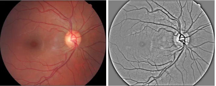
During preprocessing we extract the green plane of FPs because it provides the highest contrast between MAs and background. Since we are only interested in pixels inside a Field-of-View (FOV), we automatically generate a mask for pixels outside the FOV. A mask is generated by applying Otsu thresholding15 to the green plane of the image. Each image (I) was preprocessed (Ip) by computing a weighted sum as in Eq.1:
Ip=I·α+IGauss·β+γ (1)
wherealpha= 4 andβ =−10 are weight factors;IGauss is Gaussian blurred image that was created using filter
computed as described in Eq. 2withσ= 10;γ= 128 is a scalar added to each sum. G(x, y) = 1
2πσ2e −x2 +y2
2σ2 (2)
All values were determined experimentally. Fig.1shows an example preprocessed image.
4.2 Pixel-Wise Classification
The main goal of this stage is to classify each pixel as either MA or non-MA. The CNN is trained to map an image patch P to the corresponding annotation A(P) for all possible locations within an image. A training sample consists ofS×S sizedP andA(P) : {P, A(P)}.
L=
N X
i=1
l(A(P)i, f(Pi; Θ)) + Φ(Θ)), (3)
whereA(P)iandPiare the i-th annotation patch and i-th image patch,N is the number of training samples,
l(·) is the loss function, Θ are learning parameters, and Φ(Θ) is the regularization term.
At training time, image patches are randomly extracted using a sliding window approach with 2×2 stride. We divide image patches into MA patches containing at least 1 MA pixel and non-MA patches consisting of all remaining patches. The random artificial transformations including rotation, horizontal and vertical reflections are performed to increase variety in the training set and combat overfitting. Since we are interested in MA pixels only, the training set consists in 80% of MA patches and in 20% of non-MA patches.
At testing time, all possible image patches from inside of a FOV are extracted. To reconstruct the final image segmentation a voting mechanism is used. EachA(P) produced by the model provides a single vote for all pixels it contains. Given that patches are centred at all possible locations and theA(P) size isS×S, each pixel receives S2 votes, and a pixel receivingv votes as an MA is assigned a probability ofv/S2. As a result, a
confidence map for pixel MA membership is created.
Inspired by recent success of deep learning, we adapted a fully convolutional neural network (FCNN) to perform the pixel-wise classification between MA and non-MA pixels. Compared with the original FCNN that uses whole images as input 16 due to the small localized nature of MAs and data scarcity, we designed a network that is optimized for small image patches. Furthermore, to overcome the class imbalance problem (the overwhelming majority of pixels depicts non-MAs) we incorporated a Dice similarity coefficient function as the cost function. The training algorithm maximises the Dice loss function which measures the overlap between ground truthsyand predicted segmentation ˆy. Its values range between 0 (no overlap) and 1 (perfect agreement) and is calculated as DICE= 2∗ |y T ˆ y|+δ |y|+|y|ˆ +δ (4)
whereδis a small smoothing factor that counteracts against zero value and zero denominator.
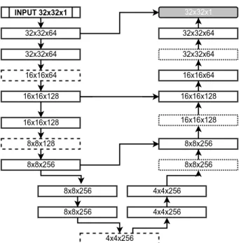
The FCNN architecture was determined experimentally and is depicted in Fig.2. It consists of 14 convo-lutional layers, each followed by a BN layer apart from the final classification layer; three 2×2 max-pooling layers and corresponding three 2×2 simple upsampling layers that replicate rows and columns of data; 3 skip connections between both paths. Double inputs in the “expanding” path are merged by concatenation. All con-volutional layers use 3×3 filters and Leaky ReLU activation function17 with 0.1 slope, apart from the final layer which uses a sigmoid activation function. Weights are updated using stochastic gradient descent with batch size 128 and Adam optimization technique18with 0.0001 initial learning rate. All training pairs are shuffled between each epoch.
4.3 Interleaved Freezing
To improve models’ generalization capabilities, we transfer the knowledge in a form of networks’ weights between models trained on different datasets and fine-tune them. Fine-tuning is a process of training a neural network from a set of pre-defined weights. A traditional approach to fine-tine deep neural networks (DNN) is to train only final layers of a network using a small learning rate. Tajbakhshet al.19 proposed a fine-tuning technique that starts from the final layer and incrementally includes more layers in the training process until a satisfactory performance is reached. Unfortunately, such an exhaustive approach is time-consuming and computationally intensive, especially for DNNs.
The DNNs are hierarchical learning models in which early layers learn low level image features and deeper layers learn more task-specific features. A learning model does not have to re-learn the low level features during a fine-tuning process, hence freezing (not training) initial layers removes redundant computations. Similarly, the final layers are the most specialized layers that require the largest weights update when the input changes. In the
Figure 2. CNN Architecture. Each block provides the shape of its output. Solid line blocks consists of a convolutional and batch normalization layers. Dashed line blocks correspond to pooling layers. Dotted line blocks represent upsampling layers. The final grey block is the final convolutional layer.
context of MA detection, two DNNs that are trained using separate datasets will learn the same general features (e.g. lesion shape) but different specific features (e.g. features related to data acquisition process such as noise or illumination changes). As such, during fine-tuning when a network is re-trained using another dataset from the same domain, we are only interested in small weight changes in most specific layers that correspond to more specific features. There is no need for computationally intensive re-training of all layers.
This paper proposes a novel fine-tuning scheme called Interleaved Freezing (IF) that takes advantage of FCNNs architecture and difference between features encoded by initial and final layers. By freezing interleaved layers we restrict the amount of weight changes in a network and the amount of trainable parameters. Compared to the approach presented by19there is no need for exhaustive iterative training process. Similarly to dropConnect regularization technique,20 the IF prevents layer co-adaptation and forces active layers to learn more robust features. Furthermore, thanks to incorporating the batch normalization layers into the FCNN, higher learning rates can be used to accelerate the learning process. Consider a FCNN with L layers
L=M+K+J+I (5)
where M, K, J, I corresponds to the number of convolutional (C), pooling (P), upsampling (U) and batch normalization (B) layers respectively. The IF is a fine-tuning scheme that freezes initial convolutional layers before the first pooling layer (P1) and freezes interleaving layers until the final upsampling layer (UJ)
Ci=
F reeze , if Ci < P1∨L−C2 i = 0∧Ci> P1∧Ci< UJ
T rain , if Ci> U1∨L−C2 i = 1∧Ci > P1∧Ci< UJ
(6) whereCi is the i-th convolutional layer.
5. EXPERIMENTAL RESULTS
To validate the proposed method we performed two sets of experiments. In the first set, we evaluate the Inter-leaved Freezing performance. In the second, we compare the performance of proposed MA detection technique with other state-of-the-art methods.
In all experiments, 20% of the training samples are held back as a validation set and an early stopping criteria is used: training stops when validation error does not improve for 20 epochs. If the validation error does not improve for 10 epochs, the learning rate is reduced by a factor of 0.3.
The implementation was based on Keras deep learning framework21 and Tensorflow numerical computation library.22 The experiments were conducted using a PC with Intel Core i7-6700K CPU, two NVIDIA TitanX graphics cards, and 64GB of RAM.
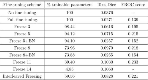
Table 1. Comparison od fine-tuning schemes.
Fine-tuning scheme % trainable parameters Test Dice FROC score No fine-tuning 100 0.0376 -Full fine-tuning 100 0.0271 0.139 Freeze 3 98.44 0.0616 0.195 Freeze 5 94.12 0.0715 0.215 Freeze 5+BN 94.10 0.0257 0.152 Freeze 8 73.96 0.0970 0.218 Freeze 8+BN 73.88 0.0255 0.154 Freeze 11 39.40 0.1030 0.233 Freeze 14 4.85 0.1060 -Interleaved Freezing 59.56 0.0828 0.221
To validate the proposed fine-tuning scheme we performed 10 experiments using ROC training dataset. For each experiment we used the same set of 25 images as a training set and 25 images as a test set. Both sets were mutually exclusive and randomly selected from ROC training dataset. The base model used for fine-tuning was trained using 354 randomly selected E-Ophtha images, and evaluated on remaining 27 images.
Table 1 shows a comparison of all fine-tuning schemes. In our experiments we applied both ”shallow” and ”deep” fine-tuning by iteratively freezing more initial layers as proposed by.19 As expected, networks trained from scratch (no fine-tuning) and fully retrained (full fine-tuning) provided worst results. The network without any fine-tuning did not produce a FROC score because the lowest average number of false positives per image (FPI) was just below 0.5, and to calculate the FROC score all seven FROC values are required. These approaches do not take full advantage of already provided knowledge in the form of a base model. We observe that by increasing the amount of frozen initial layers, our model accomplishes the best performance by freezing between 8 and 11 initial layers and training between 6 and 3 final layers. Freezing BN layers results in worse performance compared with the same models when BN layers are trainable. The network with 14 initial layers frozen achieved a comparably high test dice, however, the per-lesion evaluation showed that the lowest FPI it managed to reach was around 0.25 which is not enough to calculate a FROC score.
The Interleaved Freezing produces results comparable with the best fine-tuning scheme (0.221 vs 0.233) that required multiple experiments to obtain. A standard iterative approach requires multiple experiments to accomplish satisfactory results where the amount of experiments required grows with the amount of network’s layers. On the other hand, the IF produces competitive results with only one experiment and uses few training parameters that results in accelerated training.
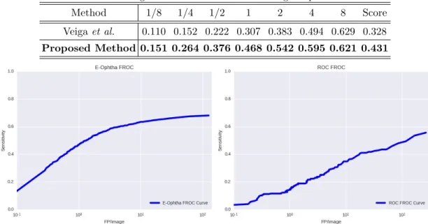
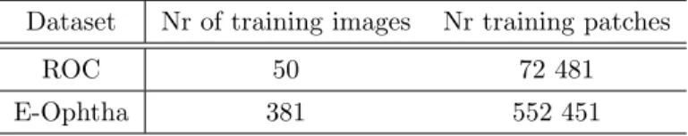
Tables 2and3present a performance comparison between the proposed method and state-of-the-art methods using ROC and E-Ophthta datasets. The proposed method achieves the highest FROC scores for both datasets. Table 4 shows the amount of training images and patches used for both experiments. Fig. 4 presents FROC curves produced by the proposed algorithm for both datasets.
Figure 3. Examples of lesion detection results for E-Ophtha dataset using 0.5 probability threshold. True positives are green circled, false positives are yellow circled and false negatives are red circled.
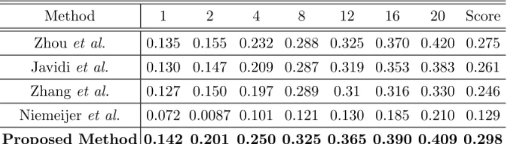
Table 2. The average sensitivies at various FPIs using ROC training dataset.
Method 1 2 4 8 12 16 20 Score Zhouet al. 0.135 0.155 0.232 0.288 0.325 0.370 0.420 0.275 Javidiet al. 0.130 0.147 0.209 0.287 0.319 0.353 0.383 0.261 Zhanget al. 0.127 0.150 0.197 0.289 0.31 0.316 0.330 0.246 Niemeijeret al. 0.072 0.0087 0.101 0.121 0.130 0.185 0.210 0.129 Proposed Method 0.142 0.201 0.250 0.325 0.365 0.390 0.409 0.298
6. DISCUSSION AND CONCLUSIONS
This paper presents a novel MA detection method evaluated using two publicly available datasets. The pro-posed algorithm uses a novel FCNN architecture with Dice coefficient loss function to segment and detect MAs. Compared to other techniques that require five computational stages, the proposed method requires only two. Furthermore, we propose a novel fine-tuning scheme called Interleaved Freezing that significantly reduces the amount of trainable parameters during network re-training and produces state-of-the-art performance.
Table 3. The average sensitivies at various FPIs using E-Ophtha dataset.
Method 1/8 1/4 1/2 1 2 4 8 Score Veigaet al. 0.110 0.152 0.222 0.307 0.383 0.494 0.629 0.328 Proposed Method 0.151 0.264 0.376 0.468 0.542 0.595 0.621 0.431
Figure 4. FROC curves produced by the proposed method for E-Ophtha and ROC training datasets.
The proposed algorithm achieves better results than state-of-the-art methods in terms of the FROC metric. As such, we think that the presented algorithm would be a useful component of a DR screening process.
ACKNOWLEDGMENTS
This research was made possible by a Marie Curie grant from the European Commission in the framework of the REVAMMAD ITN (Initial Training Research network), Project number 316990.
REFERENCES
[1] Cheung, N., Mitchell, P., and Wong, T., “Diabetic retinopathy,”Lancet376(9735), 124–36 (2010). [2] “Idf diabetes atlas, 7th edn.”,”International Diabetes Federation(2015).
[3] Guariguata, L., Whiting, D., Hambleton, I., Beagley, J., Linnenkamp, U., and Shaw, J., “Global estimates of diabetes prevalence for 2013 and projections for 2035,” Diabetes research and clinical practice103(2), 137–149 (2014).
[4] Baudoin, C., Lay, B., and Klein, J., “Automatic detection of microaneurysms in diabetic fluorescein angiog-raphy.,”Revue d’´epid´emiologie et de sant´e publique32(3-4), 254–261 (1983).
[5] Javidi, M., Pourreza, H.-R., and Harati, A., “Vessel segmentation and microaneurysm detection us-ing discriminative dictionary learnus-ing and sparse representation,” Computer Methods and Programs in Biomedicine139, 93–108 (2017).
[6] Yannuzzi, L. A., Rohrer, K. T., Tindel, L. J., Sobel, R. S., Costanza, M. A., Shields, W., and Zang, E., “Fluorescein angiography complication survey,” Ophthalmology93(5), 611–617 (1986).
[7] Walter, T., Massin, P., Erginay, A., Ordonez, R., Jeulin, C., and Klein, J.-C., “Automatic detection of microaneurysms in color fundus images,”Medical image analysis11(6), 555–566 (2007).
[8] Zhang, B., Wu, X., You, J., Li, Q., and Karray, F., “Detection of microaneurysms using multi-scale corre-lation coefficients,”Pattern Recognition43(6), 2237–2248 (2010).
[9] Veiga, D., Martins, N., Ferreira, M., and Monteiro, J., “Automatic microaneurysm detection using laws tex-ture masks and support vector machines,”Computer Methods in Biomechanics and Biomedical Engineering: Imaging & Visualization, 1–12 (2017).
[10] Decenci`ere, E., Cazuguel, G., Zhang, X., Thibault, G., Klein, J.-C., Meyer, F., Marcotegui, B., Quel-lec, G., Lamard, M., Danno, R., et al., “Teleophta: Machine learning and image processing methods for teleophthalmology,”IRBM34(2), 196–203 (2013).
Table 4. Training data.
Dataset Nr of training images Nr training patches
ROC 50 72 481
E-Ophtha 381 552 451
[11] Niemeijer, M., Van Ginneken, B., Cree, M. J., Mizutani, A., Quellec, G., S´anchez, C. I., Zhang, B., Hornero, R., Lamard, M., Muramatsu, C., et al., “Retinopathy online challenge: automatic detection of microaneurysms in digital color fundus photographs,”IEEE transactions on medical imaging29(1), 185–195 (2010).
[12] Simonyan, K. and Zisserman, A., “Very deep convolutional networks for large-scale image recognition,”
arXiv preprint arXiv:1409.1556(2014).
[13] Long, J., Shelhamer, E., and Darrell, T., “Fully convolutional networks for semantic segmentation,” in [Proceedings of the IEEE Conference on Computer Vision and Pattern Recognition], 3431–3440 (2015). [14] Krizhevsky, A., Sutskever, I., and Hinton, G. E., “Imagenet classification with deep convolutional neural
networks,” in [Advances in neural information processing systems], 1097–1105 (2012).
[15] Otsu, N., “A threshold selection method from gray-level histograms,”IEEE transactions on systems, man, and cybernetics9(1), 62–66 (1979).
[16] Ronneberger, O., Fischer, P., and Brox, T., “U-net: Convolutional networks for biomedical image segmen-tation,” in [International Conference on Medical Image Computing and Computer-Assisted Intervention], 234–241, Springer (2015).
[17] Maas, A. L., Hannun, A. Y., and Ng, A. Y., “Rectifier nonlinearities improve neural network acoustic models,” in [Proc. ICML],30(1) (2013).
[18] Kingma, D. and Ba, J., “Adam: A method for stochastic optimization,” arXiv preprint arXiv:1412.6980
(2014).
[19] Tajbakhsh, N., Shin, J. Y., Gurudu, S. R., Hurst, R. T., Kendall, C. B., Gotway, M. B., and Liang, J., “Convolutional neural networks for medical image analysis: full training or fine tuning?,”IEEE transactions on medical imaging35(5), 1299–1312 (2016).
[20] Wan, L., Zeiler, M., Zhang, S., Le Cun, Y., and Fergus, R., “Regularization of neural networks using dropconnect,” in [International Conference on Machine Learning], 1058–1066 (2013).
[21] Chollet, F. et al., “Keras.” https://github.com/fchollet/keras(2017).
[22] Abadi, M., Agarwal, A., Barham, P., Brevdo, E., Chen, Z., Citro, C., Corrado, G. S., Davis, A., Dean, J., Devin, M., et al., “Tensorflow: Large-scale machine learning on heterogeneous distributed systems,”arXiv preprint arXiv:1603.04467(2016).