Testing for Parameter Instability in Predictive Regression Models

Essex Finance Centre

Working Paper Series

Working Paper No29: 01-2018

Testing for Parameter Instability in Predictive

Regression Models

“Iliyan Georgiev, David I. Harvey, Stephen J. Leybourne

and A.M. Robert Taylor”

Essex Business School, University of Essex, Wivenhoe Park, Colchester, CO4 3SQ Web site: http://www.essex.ac.uk/ebs/

Testing

for

Parameter

Instability

in

Predictive

Regression

Models

IliyanGeorgieva, DavidI. Harveyb, StephenJ. Leybourneb

and A.M. RobertTaylorc

a_{Department ofStatisticalSciences, Universitàdi Bologna} b _{SchoolofEconomics, Universityof Nottingham}

c_{EssexBusinessSchool,UniversityofEssex}

Abstract

We consider tests for structural change, based on theSupF and Cramer-von-Mises type statistics of Andrews (1993) and Nyblom (1989), respectively, in the slope and/or intercept parameters of a predictive regression model where the predictors display strong persistence. The SupF type tests are motivated by alternatives where the parameters display a small number of breaks at deterministic points in the sample, while the Cramer-von-Mises alter-native is one where the coe¢ cients are random and slowly evolve through time. In order to allow for an unknown degree of persistence in the predictors, and for both conditional and unconditional heteroskedasticity in the data, we implement the tests using a …xed regressor wild bootstrap procedure. The asymptotic validity of the bootstrap tests is established by showing that the asymptotic distributions of the bootstrap parameter constancy statistics, conditional on the data, coincide with those of the asymptotic null distributions of the cor-responding statistics computed on the original data, conditional on the predictors. Monte Carlo simulations suggest that the bootstrap parameter stability tests work well in …nite samples, with the tests based on the Cramer-von-Mises type principle seemingly the most useful in practice. An empirical application to U.S. stock returns data demonstrates the practical usefulness of these methods.

Keywords: Predictive regression; persistence; parameter stability tests; …xed regressor wild bootstrap; conditional distribution.

JEL Classi…cation: C12, C32, C58.

We are very grateful to the Co-Editor, Oliver Linton, an Associate Editor and three anonymous referees for their helpful and constructive comments on earlier versions of this paper. Taylor gratefully acknowledges …nancial support provided by the Economic and Social Research Council of the United Kingdom under research grant ES/R00496X/1. Correspondence to: Robert Taylor, Essex Business School, University of Essex, Wivenhoe Park, Colchester, CO4 3SQ, United Kingdom. Email:[email protected].

1

Introduction

Predictive regression (hereafter PR) is a widely used tool in applied …nance and economics. A leading example concerns whether future stock returns can be predicted by current infor-mation. In this context PR methods have been extensively utilised in studies of mutual fund performance, tests of the conditional CAPM and studies of optimal asset allocation; see Paye and Timmermann (2006,pp.274-275) and references therein. Predictors commonly considered for returns include the dividend yield, the term structure of interest rates, and default premia. It is often found that the posited predictor (e.g. the dividend yield) exhibits strongly persistent behaviour akin to that of a (near-) unit root autoregressive process, whilst the variable being predicted (e.g. the stock return) resembles a (near-) martingale di¤erence sequence [m.d.s.].

Predictability tests which are asymptotically valid when the putative predictor is strongly persistent and driven by innovations which are correlated with the series being predicted (the latter is often thought to be the case; e.g., the stock price is a component of both the return and the dividend yield) have been proposed in Cavanaghet al. (1995), Campbell and Yogo (2006), Kostakiset al. (2015), Breitung and Demetrescu (2015), Elliottet al. (2015) and Jansson and Moreira (2006),inter alia. These approaches are all based on the maintained assumption that the coe¢ cients of the PR model are constant over time. There is, however, a growing body of empirical evidence casting doubt on this assumption. Henkelet al. (2011), for example, …nd that return predictability in the stock market appears to be closely linked to economic recessions with dividend yield and term structure variables displaying predictive power only during recessions. Johanneset al. (2014) …nd strong empirical evidence of time-variation in the parameters of PRs for returns, including evidence of non-constant volatility. Timmermann (2008) argues that for most time periods stock returns are not predictable but that there are ‘pockets in time’where evidence of local predictability is seen. Paye and Timmermann (2006) also cite a number of applied studies which …nd signi…cant evidence of in-sample (ex post) predictability in returns data but yet …nd very weak evidence of out-of-sample (ex ante) predictability, and argue that a possible explanation is structural instability in the predictive relations involved.

Paye and Timmermann (2006) use a variety of well-known structural change tests designed against abrupt (deterministic) changes in a model’s parameters to investigate the structural stability of PRs for stock returns related to structural breaks in the coe¢ cients of state variables (including the lagged dividend yield, short interest rate, term spread and default premium) for a data-set of monthly stock returns for ten OECD countries. They …nd evidence of instability for the vast majority of these countries, arguing that the “Empirical evidence of predictability is not uniform over time and is concentrated in certain periods.”op.cit. p.312. They also present simulation evidence into the size and power of the structural change tests they consider for the case where the predictors involved are I(0) and a one-time break is allowed in the coe¢ cient on a single predictor, and conclude in favour of the approach of Bai and Perron (1998,2003). A signi…cant drawback of applying the Bai and Perron approach to the PR model, however, is that it is not asymptotically valid in cases where the predictive variables are (near-) unit root

processes. Moreover, as argued by Caiet al. (2015,p.954) and the references therein, its focus on models of abrupt deterministic coe¢ cient change might be considered unattractive in practice relative to tests designed for the case where the parameters of the PR are random and evolve smoothly over time. Indeed, using Bayesian model selection and averaging methods, Dangl and Halling (2012) conclude that time-variation in the coe¢ cients of return prediction models is very important with a random walk coe¢ cients model performing best in practice, quickly adapting to changes in environment. They also …nd evidence suggestive that predictability is linked to the business cycle. The Bai and Perron approach also requires that the variables in the PR do not display unconditional heteroskedasticity which would again appear to considerably limit their applicability for …nancial data; see, e.g., Johannes et al. (2014).

Our aim here is to address these shortcomings and develop structural change tests that can be more reasonably applied to empirically testing the constancy of the intercept and slope parameters in a PR model driven by heteroskedastic innovations. In earlier work, Georgiev et al. (2018) [GHLT hereafter], we investigated a variant of the stationarity test of Kwiatkowski et al. (1992) [KPSS] in the context of the PR model. This is a test of the instability of the regression intercept and can be viewed as a test against the alternative that the error in the PR model follows a near-unit root process. As such, GHLT interpret this as a test for spurious predictability. The present paper extends the work in GHLT to cover tests on all or a subset of the parameters of the PR model, not just the intercept, thereby allowing us to also investigate the constancy or otherwise of the slope parameter on the predictive regressor.

In the light of the arguments above, we consider parameter constancy tests based on the SupF type statistics of Andrews (1993) and the Cramer-von-Mises type statistics of Nyblom (1989). The former are designed for abrupt deterministic change models and the latter for (near-) unit root coe¢ cient models. Although originally developed forasymptotically stationary regressors, Hansen (1992a) examines the large sample properties of these statistics for the case of pure unit root regressors, showing how these limits di¤er from the asymptotically stationary case. However, in the context of the PR model we need to go further and allow for the case where the predictive regressor is a near-unit root processes. Doing so introduces the considerable complication relative to the case of a pure unit root regressor that the limiting null distributions of the parameter constancy statistics depend on the local-to-unity (persistence) parameter of the putative predictor. In principle, this makes it very di¢ cult to control the size of the tests given that this parameter is unknown in practice and cannot be consistently estimated.1

To resolve this problem we use bootstrap implementations of the parameter constancy tests which treat the putative predictor as a …xed regressor; i.e., the observed data on the predictor is used in calculating the bootstrap analogues of the structural change statistics. Because, as noted above, many economic and …nancial time series are thought to display non-stationary volatility and/or conditional heteroskedasticity, it is also important for our proposed bootstrap tests to

1

Caiet al. (2015) also develop a test against smooth parameter variation in the parameters of the PR model based on a non-parametric L2-type statistic. However, their proposed statistic requires the variables in the

be (asymptotically) robust to these e¤ects. To achieve this we use a heteroskedasticity-robust variant of the …xed regressor bootstrap approach proposed in Hansen (2000). We show that this approach yields asymptotically size-controlled tests, without requiring knowledge of the local-to-unity parameter or the form of any heteroskedasticity present, and delivers tests which are powerful against both forms of coe¢ cient variation considered. Moreover, the bootstrap tests are also valid when the predictive regressors are asymptotically stationary or contain a mix of both asymptotically stationary and strongly persistent regressors. They are also valid for regressors whose marginal distributions are subject to structural change, meaning that rejection by the bootstrap tests can be unambiguously interpreted as evidence for structural instability in the slope coe¢ cients of the PR, even where the predictors themselves display structural change. Closely related to this paper, Hansen (2000) also applies the …xed regressor bootstrap to the Andrews (1993) and Nyblom (1989) statistics we consider here, and Paye and Timmermann (2006) include the …xed regressor bootstrap implementation of the Andrews (1993) test in their simulation study. Although Hansen (2000) employs assumptions that allow for pure and near unit root behaviour in the regressor variables, we demonstrate that his formal analysis needs an amendment. Hansen (2000) justi…es bootstrap validity by claiming equivalence of the limiting distribution of the bootstrap parameter constancy statistics given the data and the unconditional limiting distribution of the original test statistics under the null. We show that this equivalence does not occur; in particular, the limits of the bootstrap statistics in his Theorems 5 and 6 on page 107 are both imprecisely stated when the predictive regressors are (near-) unit root processes. We establish that the …xed regressor bootstrap is nevertheless valid, at least in the PR set-up we consider, in the sense that the bootstrap parameter instability tests are asymptotically size-controlled. This is done by demonstrating that the limiting distributions of the bootstrap statistics, conditional on the data, are the same as the limiting null distributions of the corresponding statistics computed on the original data, conditional on the predictors.

The paper is organised as follows. Section 2 outlines our basic time-varying parameter PR model. To aid lucidity, we expound our approach through a single predictor variable whose innovations are serially uncorrelated. Generalisations to allow for multiple predictors and weak dependence are discussed in section 6. Section 3 outlines the structural change statistics and derives their asymptotic distributions. Section 4 details the …xed regressor wild bootstrap tests based on these statistics and establishes their asymptotic validity. The asymptotic local power of the bootstrap tests is examined in section 5, while section 7 presents Monte Carlo simulation results investigating their …nite sample performance. An empirical application to monthly U.S. stock returns data is presented in Section 8. Section 9 concludes. Proofs appear in an appendix. Additional material relating to the limiting distributions of the statistics given in section 3 is provided in an accompanying on-line supplementary appendix.

2

The Predictive Regression Model with Structural Change

The basic PR model allowing for structural change that we consider for observed ytis given by

yt= t+ txt 1+ yt; t= 1; :::; T (1)

wherextis an observed process, speci…ed according to the data generating process [DGP]

xt= +sxt; t= 0; :::; T (2)

sxt= xsxt 1+ xt; t= 1; :::; T (3)

where _x:= 1 cxT 1 withcx 0such thatxtis a strongly persistent unit root or local-to-unit

root autoregressive process with mean zero innovation process xt. We let sx0 be an Op(1)

variate. Exact conditions on the innovations yt and xt will be given in Assumption 1 below.

The DGP in (1) generalises the constant parameter PR model by allowing the intercept and slope coe¢ cients to vary over time. To nest the constant parameter PR within (1) we formulate the time-varying intercept and slope coe¢ cients as: t := ( +as t) and t := ( +bs t).

The parameter instability tests we discuss in this paper are, by construction, invariant to the values of and . However, in the context of a time-invariant PR (i.e., t = , t = ) with

near-unit root predictors it is usual to follow Cavanaghet al. (1995) and parameterise to be local-to-zero at an appropriate rate; precisely, =gT 1 wheregis some constant. This entails that under parameter constancy, and when g is non-zero, yt is a near-m.d.s. process. Where

is …xed, as in Shin (1994), (1) should rightly be interpreted as a co-integrating regression becauseytwill be a (near-) unit root process. However, because no particular parameterisation

is needed for the theoretical results which follow (only for the PR interpretation of (1)) we do not directly impose a localisation on . This is because in the case wherext is (asymptotically)

stationary no such standardisation of is needed for a PR interpretation of (1).

In the context of (1) our focus will centre on testing the null hypotheses that the intercept and slope parameters are constant over time against the alternative that they vary over time through the sequences of associated time-varying coe¢ cients, s tand s t. This can be done by

testing the restrictions thata= 0 and b= 0 in (1). We will consider two possible mechanisms.

S: Stochastic Coe¢ cient Variation

The …rst mechanism we consider for time variation in t and tin (1), in the spirit of Nyblom

(1989), is one wheres t and s t follow (near-) unit root processes. That is, " s t s t # = " 0 0 # " s t 1 s t 1 # + " t t # (4)

where := 1 c T 1, := 1 c T 1 withc 0,c 0which are unit root or local to unit root autoregressive processes.2 Precise m.d.s.-based assumptions on the innovations tand t

will be given in Assumption 1. The coe¢ cient processes are initialised ats 0 =s 0 = 0.

2

For (1) to be interpreted as a PR the parameterashould, paralleling the discussion surrounding above, be localised asa=g T 1_{under (4), otherwisey}

In the context of (4), the PR in (1) reduces to a …xed coe¢ cient model when a = 0 and

b= 0. The intercept alone is random if a₆= 0while b= 0. In this situation, if (1) is treated as a …xed coe¢ cient regression model, it is then under-speci…ed by an unobserved (local to) unit root autoregressive process; this is akin to the omission of a valid (local to) unit root predictive regressor, as studied in GHLT. Ifa= 0 whileb₆= 0, treating (1) as a …xed coe¢ cient regression model ignores the fact that the relationship betweenyt and the predictive regressorxt 1 is not

stable but is evolving through time. If a ₆= 0 and b ₆= 0, then both forms of mis-speci…cation are present together when (1) is assumed to be a …xed coe¢ cient model. In terms of hypothesis testing, then, we summarise these possibilities via the following taxonomy covering the null,

H0, and various alternatives,HS, in the context of (1) and (4):

H0 : a= 0; b= 0 both intercept andxt 1 slope coe¢ cient are …xed

HS

1 : a6= 0; b= 0 intercept only varies

H_xS : a= 0; b₆= 0 xt 1 slope coe¢ cient only varies

H₁S_x : a₆= 0_[b₆= 0 either the intercept or xt 1 slope coe¢ cient, or both, vary.

N: Non-stochastic Coe¢ cient Variation

The second mechanism we consider for time variation in tand tin (1) follows, among others,

Andrews (1993) and is one where they are subject to abrupt changes which occur at a …xed number of deterministic points in the sample. For simplicity we will expound our analysis through the case of a one-time break, although the extension to allow for multiple such breaks is straightforward. However, where it is thought that multiple breaks are possible, the stochastic coe¢ cient variation case might be considered a more natural framework; see also Remark 3 below. In the one-time break cases t and s t are modelled as

s t=s t=Dt(b 0Tc) (5)

whereDt(b Tc) :=I(t >b Tc) with b Tcdenoting a generic shift point with associated break

fraction ,_{b c}the integer part of its argument and _I(:)the indicator function. We take the true shift fraction 0 as unknown to the practitioner but to satisfy 0 2 , where = [ L; U]with

0< L < U <1. Here then, at time b 0Tc, the intercept changes value from to +a; the

coe¢ cient on xt 1 changes value from to +b. The corresponding taxonomy covering the

null, H0, and various alternatives,HN, in the context of (1) and (5) is then:

H0 : a= 0; b= 0 both intercept andxt 1 slope coe¢ cient are …xed

H₁N : a₆= 0; b= 0 intercept only shifts

H_xN : a= 0; b₆= 0 xt 1 slope coe¢ cient only shifts

H₁N_x : a₆= 0_[b₆= 0 either the intercept or xt 1 slope coe¢ cient, or both, shift.

We conclude this section by detailing in Assumption 1 the conditions that we will place on the innovation vector t := [ xt; yt; t; t]0 in what follows, noting that only the assumptions

pertaining to the leading two elements of tare germane under schemeN. Some remarks follow.

(a) H and Dt are the 4 4 non-stochastic matrices H := 2 6 6 6 6 6 4 1 0 0 0 h21 1 0 0 h31 h32 1 0 h41 h42 h43 1 3 7 7 7 7 7 5 ; Dt:= 2 6 6 6 6 6 4 d1t 0 0 0 0 d2t 0 0 0 0 d3t 0 0 0 0 d4t 3 7 7 7 7 7 5

with hij 2R;(i= 2;3;4, j= 1;2;3), such that HH0 is strictly positive de…nite. The volatility

terms dit satisfy dit = di(t=T), where di( ) _{2 D}, _Dk := Dk[0;1] denoting the space of right

continuous with left limit (càdlàg) _Rk-valued functions on [0;1] equipped with the Skorokhod topology, are non-stochastic, strictly positive functions.

(b) et is a 4 1 vector m.d.s. with respect to a …ltration Ft, to which it is adapted, with

conditional covariance matrix t:= E(ete0tjFt 1) satisfying: (i) T 1PTt=1 t

p

! E(ete0_t) = I4,

p

! denoting convergence in probability as T _{! 1}, and (ii) sup_tE_ke_tk4+ <₁ for some >0, where for any vector, x, _kx_k denotes the usual Euclidean norm,_kx_k:= (x0_x)1=2_.

Remark 1. Assumption 1 implies that t is a vector m.d.s. relative to Ft, with conditional

variance matrix tjt 1 :=E( t 0tjFt 1) = (HDt) t(HDt)0, and time-varying unconditional

vari-ance matrix t:=E( t 0t) = (HDt)(HDt)0>0.3 Stationary conditional heteroskedasticity and

non-stationary unconditional volatility are obtained as special cases withdi( ) =di,i= 1;2;3;4 (constant unconditional variance, hence only conditional heteroskedasticity), and t = I4 (so

tjt 1 = t= (t=T), only unconditional non-stationary volatility), respectively. Assumption

1(a) implies that the elements of tare only required to be bounded and to display a countable

number of jumps, therefore allowing for a wide class of models for the behaviour of the variance matrix of t(subject to the structure imposed byH), including single or multiple (co-) variance

shifts, variances which follow a broken trend, and smooth transition variance shifts. Assumption 1(b) coincides with the m.d.s. conditions in Assumption 1 of Breitung and Demetrescu (2015), except that the cross product moment summability condition given there is not required as we do not allow xt to be serially correlated at this stage. We will discuss extensions to allow for

this in section 6.1 where a corresponding condition will be introduced. Deo (2000) provides examples of commonly used stochastic volatility and generalised autoregressive-conditional het-eroskedasticity (GARCH) processes that satisfy Assumption 1(b).

Remark 2. Assumption 1 permits correlation between the elements of tthrough the elements

hij, i = 2;3;4, j = 1;2;3, of the matrix H. In particular, where h21 6= 0, then yt and the

innovations drivingxt, xt, are correlated.

Remark 3. Wherec =c = 0 such that = = 1, Assumption 1 entails that [s t; s t]0 is

a martingale of the form considered in Equation (2.1) of Nyblom (1989,p.224). This permits t

and _t to undergo either a deterministic or a random number of jumps of random magnitude,

3_{Notice that the assumptions thatE(e}

te0t) =I4 made in part (b)i and that the leading diagonal elements of H are unity involve no loss of generality.

with the number of jumps remaining (on average) a non-vanishing fraction of the sub-sample size, in every sub-sample. Where the (expected) number of jumps is lower than the sample size, they occur at random points in the sample. Moreover, as we allow t and t to display

non-constant unconditional variances these jumps can be such that they are much more likely to occur in certain parts of the sample than others allowing for clustering of the jumps. Where

c > 0; c > 0, [s t; s t]0 is a near-martingale and the coe¢ cient processes t and t display

long run mean reversion (towards and respectively).

3

Parameter Constancy Tests

We …rst outline the structural change statistics that we will consider for testing parameter constancy in the PR in (1). We will then establish the large sample properties of these statistics.

3.1 Structural Change Test Statistics

S: Stochastic Coe¢ cient Variation

To test H0 againstHS we adopt the LM statistic of Nyblom (1989). Under certain conditions,

including homoskedasticity and the requirement that = = 1 in (4), then, conditional on

xt, this test statistic has a Locally Best Invariant (LBI) property. For testing H0 against H1Sx,

the relevant LM statistic is given by

LM1x:= 1 T^2 T X i=1 i X t=1 a0_t^et ! _T X t=1 ata0t ! 1 _i X t=1 atet^ ! (6)

whereat:= [1xt 1]0, with^2 :=T 1PT_t=1^e2t, with^etthe OLS residual from the …tted regression

yt= ^ + ^xt 1+ ^0 xt+ ^et; t= 1; :::; T: (7)

As in Shin (1994), (7) contains the additional regressor xt, to account for the possibility of a

non-zero correlation between xt and yt (which occurs when h21 6= 0 in Assumption 1). The

same will be needed in the context of the SupF statistics considered below.

We can also consider the corresponding single parameter LM statistics. These are given by

LM1:= 1 T2_^2 T X i=1 i X t=1 ^ et !2 and LMx:= 1 (T^2PT_t=1x2_{t 1}) T X i=1 i X t=1 xt 1et^ !2 (8)

for the test statistics relating to the intercept alone and to the slope coe¢ cient alone, respec-tively. ThereforeLM1 is appropriate for testingH1S, whileLMx is appropriate for testingHxS.

The LM1 statistic coincides with the statistic proposed in GHLT.

N: Nonstochastic Coe¢ cient Variation

To testH0 againstHN we use the SupF statistic of Andrews (1993). In a rather general, but

certain weak asymptotic local optimality properties against this form of parameter variation. For testingH0 against H1Nx in (1) and (5), this statistic is given by

SupF_1x:= sup

2

F( ); F( ) :=T^

2 _^2_{( )}

^2( ) (9)

with ^2 de…ned as above, and ^2( ) :=T 1PT

t=1e^2t( ),^et( )from the …tted OLS regression

yt= ^ + ^ Dt(b Tc) + ^xt 1+ ^ Dt(b Tc)xt 1+ ^0 xt+ ^et( ); t= 1; :::; T: (10)

To test againstHN

1 , exclude Dt(b Tc)xt 1 from (10); denote the resulting statistic by SupF1.

For testing againstH_xN,Dt(_b T_c)is excluded from (10), and we denote this statistic bySupFx.

Remark 4. The LM andSupF statistics are used to test the same null hypothesis,H0, but di¤er

in which alternative hypothesis they are directed towards. Still, as Hansen (1992a,p.325) points out they will “...tend to have power in similar directions...”The numerical results reported later in this paper accord with this view. Hansen argues that, as a result, the choice between the tests might be made on computational grounds and argues that this favours the LM statistic. He also argues that the purpose of the test is important and that if one is looking to test against a rapid change in regime then theSupF statistics would be appropriate, while “...if one is simply interested in testing whether or not the speci…ed model is a good model that captures a stable relationship, the notion of martingale parameters is more appropriate, since it captures the notion of an unstable model that gradually shifts over time.”op. cit. p.325.

3.2 Asymptotic Distribution Theory

Under Assumption 1, the conditions of Lemma 1 of Boswijket al. (2016) are satis…ed such that

T 1=2 bTc X t=1 t; T 1 T X t=1 t 1 X s=1 s 0t ! w ! M ( ); Z 1 0 M (s)dM (s)0 (11)

where_!w denotes weak convergence asT _{! 1}, andM ( ) := [M x( ); M y( ); M ( ); M ( )]0

is a Gaussian martingale satisfying

2 6 6 6 6 6 4 M x( ) M y( ) M ( ) M ( ) 3 7 7 7 7 7 5 := H 2 6 6 6 6 6 4 R 0d1(s)dB1(s) R 0d2(s)dB2(s) R 0d3(s)dB3(s) R 0d4(s)dB4(s) 3 7 7 7 7 7 5 = 2 6 6 6 6 6 4 fR01d21(s)g1=2 0 0 0 h21fR₀1d12(s)g1=2 f R1 0 d 2 2(s)g1=2 0 0 h31f R1 0 d 2 1(s)g1=2 h32f R1 0 d 2 2(s)g1=2 f R1 0 d 2 3(s)g1=2 0 h41f R1 0 d21(s)g1=2 h42f R1 0 d22(s)g1=2 h43f R1 0 d23(s)g1=2 f R1 0 d24(s)g1=2 3 7 7 7 7 7 5 2 6 6 6 6 6 4 B 1( ) B 2( ) B 3( ) B 4( ) 3 7 7 7 7 7 5

with B i( ) := fR₀1d2_i(s)g 1=2R₀di(s)dBi(s), i = 1;2;3;4, and [B1( ); B2( ); B3( ); B4( )]0 a

standard Brownian motion in _R4. We can also write B i( ) d

i( ) denotes the variance pro…le i( ) :=f R1 0 d 2 i(s)g 1 R 0d 2 i(s)ds,i= 1;2;3;4, such that B i( )

is a variance-transformed Brownian motion; see, for example, Davidson (1994, p.484). Under unconditional homoskedasticity, _i(s) =s.

It will also prove convenient to de…ne the Ornstein-Uhlenbeck [OU] type processesB 1;cx(r) := Rr 0 e (r s)cxdB 1(s), M ;c ( ) := Rr 0 e (r s)c dM (s) and M ;c ( ) := Rr 0 e (r s)c dM (s),

for r ₂ [0;1], along with M x;cx( ) := f R1

0 d

2

1(s)dsg1=2B 1;cx( ) and its de-meaned analogue, M x;cx( ) :=M x;cx( )

R1

0 M x;cx(s)ds.

In order to examine the asymptotic local power properties of the tests we discuss we will specify HS and HN as local to H0 by normalising the parameters a and b to be

local-to-zero. The relevant normalisations are di¤erent for aand b and di¤er according to which form of coe¢ cient variability is being considered. Speci…cally, under scheme S these are given by

a=g T 1 in H₁S and H₁S_x and b =g T 3=2 in H_xS and H₁S_x, while under scheme N these are given by a=g T 1=2 inH₁N and H₁N_x and b=g T 1 inH_xN and H₁N_x. In each caseg and g

are …xed Pitman drift constants. Notice also that in these local settings HS _{and H}N _{reduce to} H0 when g =g = 0. In what follows, reference to these alternative hypotheses is understood

to be made under these localisations, unless otherwise stated.

We now provide representations for the asymptotic distributions of the LM andSupF statis-tics under the local alternatives stated above. In Theorem 1 we do this for LM1x and SupF1x

in terms of matrix-valued processes. Alternative expressions for these limiting distributions in terms of scalar processes, together with those for the single parameterLM1,LMx,SupF1 and

SupFx statistics are provided in the on-line supplement.

Theorem 1. Consider the model in (1), (2), (3) and let Assumption 1 hold. Then under the

null hypothesis and the local alternatives outlined above,

LM1x!w Z 1 0 J0(r)_fV(1)_g 1J(r)dr SupF_{1x !}w sup r2 J(r)0_fV(r) V(r)V(1) 1V(r)_g 1J(r) ;

whereJ(r) :=R₀rA(s)dY (s) V(r)V(1) 1R₀1A(s)dY (s)andV(r) :=R₀rA(s)A0(s)dswith

A(r) := [1; M x;cx(r)]0 and Y (r) :=B 2(r) +

nR1

0 d22(s)ds

o 1=2R_r

0 Q(s)ds. Finally, the process

Q(r),r ₂[0;1] is de…ned such that Q(r) :=g M ;c (r) +g M ;c (r)M x;cx(r) under scheme S, while under under scheme N, Q(r) :=_fg +g M x;cx(r)gI(r 0).

Remark 5. The limit expressions given in Theorem 1 for the LM1x and SupF1x statistics can

be regarded as statistics of theLM andSupF type, respectively, in the context of a continuous-time least squares regression of dY (r) on dr and M x;cx(r)dr. Under the null hypothesis of

parameter stability, Q(r) = 0 for all r in these representations, while under the alternative hypotheses considered, the presence of parameter instability a¤ects the limit distributions of both test statistics through the process Q( ) which is a function of the Pitman drifts, g and

g . Although motivated under speci…c forms of instability, both statistics can therefore be seen to be sensitive to both of the considered alternatives.

Remark 6. The representations in Theorem 1 for the limiting distributions of LM1x and

SupF1x depend, under both the null,H0, and the local alternatives considered, on the

local-to-unity parameter, cx, characterising the degree of persistence in xt. For LM1x this dependence

can be seen more clearly in the alternative representation of its limiting distribution in Corollary S.1 in the supplement. ForSupF1x, consider for simplicity the benchmark case of unconditional

homoskedasticity in t; and observe …rst that the limiting processes J( ), V( ) and Q( ) all

depend on cx. Under H0, for …xed r 2 , dependence oncx disappears from the distribution

of _fV(r) V(r)V(1) 1V(r)_g 1=2J(r) =d N(0; I2), both conditionally on fA(s)gs₂[0;1] and

unconditionally, because in this case J( )conditional on _fA(s)_gs2[0;1] is a zero-mean Gaussian process with covariance function E_fJ(r1)J0(r2)jfA(s)gs₂[0;1]g= V(r1) V(r1)V(1) 1V(r2)

forr1 r2. It follows that the limiting null distribution ofF( ) from (9) under unconditional

homoskedasticity is 2(2) regardless of whether xt 1 is a pure unit root (cx = 0), a

near-unit root (cx > 0), or even an asymptotically stationary process (see Andrews, 1993, for the

latter). However, upon taking the supremum over r ₂ , the distribution of the resulting functional SupF1x conditional on fA(s)gs₂[0;1] depends on all the conditional covariances of

fV(r) V(r)V(1) 1V(r)_g 1=2J(r) and not just on its trivial conditional variance, and so depends oncx. This dependence carries over to the unconditional distribution of SupF1x.

Remark 7. It can also be seen from the representations given in Theorem 1 that the

lim-iting distributions of the structural change statistics do not depend on any of the elements of the matrix H in Assumption 1, under either the constant parameter null hypothesis, H0,

or the local alternatives involving non-stochastic coe¢ cient variation N. They do, however, depend on any unconditional non-stationary volatility present in the innovations through the variance transformed Brownian motionB 2(r)and the scaled variance transformed OU process

M x;cx(r); that is, from any unconditional heteroskedasticity present in yt and xt. Where the

local alternatives pertain to the stochastic coe¢ cient variation scheme S in (4), these limiting distributions also depend on any unconditional heteroskedasticity present in t when g 6= 0

and in t when g 6= 0, and on the correlation between yt; xt and t; t:

Remark 8. The representations given in Theorem 1 …t with the generic representations given in

Theorem 2 of Hansen (2000). Hansen (2000,p.98) gives a set of high-level conditions governing the weak convergence of the sample moments of the data and gives representations for the limiting distributions of the statistics under those conditions. The model set-up with associated assumptions that we consider here is, in the benchmark case of unconditional homoskedasticity in tand of no correlation between ytand xt(i.e.,h21= 0);an example which satis…es Hansen’s

conditions and so we would expect our result to accord with his generic result. This is indeed seen to be so on noting that the processesV( ) andR₀A(s)dY (s)which appear in Theorem 1 coincide with the genericM( )andN( )processes, respectively, in Theorem 2 of Hansen (2000) under the speci…c conditions of the benchmark case outlined above.

Remark 9. Where xt 1 is asymptotically stationary (in the sense of De…nition 1 of Hansen,

and SupF1x statistics are, by Theorem 1 of Hansen (2000), of the form given in Equation (3.3)

of Nyblom (1989,p.226) and Theorem 3 of Andrews (1993,p.838), respectively. More gener-ally, consider the case where T 1Pb_t=1T c[1; xt 1]0[1; xt 1] and T 1P_tb₌₁Tc[1; xt 1]0[1; xt 1]d22te22t, r ₂[0;1], converge in probability to deterministic processes (say, Ve( ) and _fR₀1d2₂(s)_g1=2Ve ( ), respectively), which are continuous and, for r > 0, positive de…nite. Further suppose that

T 1=2Pb_t=1T c[1; xt 1]0d2te2t converges weakly to a zero-mean Gaussian process (say, Je0( )) with

independent increments and variance function _fR₀1d2

2(s)g1=2Ve ( ), and let xt 1 be such that

the inclusion of xt in (7) eliminates the e¤ects of h21d1te1t from the residual, ^et. Then the

asymptotic null distributions of the LM1x and SupF1x statistics are as given in Theorem 1,

but with Je0 and Ve replacing J and V, respectively.4 The dependence of these distributions

on (among other things) heteroskedasticity introduced by a general function d2( ) of the form

given in Assumption 1 would make the use of a bootstrap approximation desirable and, by the arguments of Theorems 5 and 6 of Hansen (2000), the …xed regressor wild bootstrap we outline in section 4 would be asymptotically valid. Because in this case the …xed regressor bootstrap statistics would converge to non-random distributions, the focus on conditioning which char-acterises the central results of this paper for the case of strongly persistent regressors becomes unnecessary. However, the key point is that the …xed regressor wild bootstrap implementations of the structural change tests we consider will be asymptotically valid regardless of whether

xt satis…es the conditions outlined in section 2 (the proof of which is given in section 4.1) or

the generic conditions outlined above, and can therefore be validly used regardless of which of these two set-ups holds for xt, or, when allowing for multiple predictors (see section 6.2), the

case where both types are present; indeed, they are also asymptotically valid in cases where the degree of persistence of the variables in xt changes over the sample. Moreover, as

demon-strated in Theorems 5 and 6 of Hansen (2000), the …xed regressor bootstrap tests will also be asymptotically valid if the set of predictors includes regressors whose marginal distributions are subject to structural change of the form given in Section 4 of Hansen (2000).

4

Fixed Regressor Wild Bootstrap Tests

As the results in the previous section show, implementing tests based on the LM and SupF statistics will require us to address the fact that their limiting null distributions depend on any unconditional heteroskedasticity present in xtand yt, and on the persistence parametercx. To

account for the former we employ a wild bootstrap procedure based on the residuals et^ of the …tted regression (7), while for the latter we use the observed outcome onx:= [x0; x1; :::; xT]0 as

a …xed regressor when implementing the bootstrap procedure.

We now outline our …xed regressor wild bootstrap approach in Algorithm 1. To aid expo-sition we do so for the bootstrap tests based on the LM1x statistic, but it should be entirely

clear how the same approach can be applied to the LM1, LMx, SupF1x, SupF1 and SupFx 4

The corresponding limiting distributions under local alternatives can be obtained by appropriately modifying the limiting processQ( )in Theorem 1.

statistics, with the resulting bootstrap analogues of these statistics correspondingly denoted by LM₁,LM_x,SupF_1x,SupF₁ and SupF_x, respectively.

Algorithm 1 (Fixed Regressor Wild Bootstrap):

(i) Construct the wild bootstrap innovations y_t := wte^t, where wt, t = 1; : : : ; T, is an IID N(0;1)sequence independent of the data.

(ii) Calculate the …xed regressor wild bootstrap analogue ofLM1xas outlined in section 3, but

withy_t in place ofytand with the regressor xtomitted. Denote the resulting bootstrap statistic asLM_1x.

(iii) De…ne the correspondingp-value asP_T := 1 G_T(LM_1x), withG_T( )denoting the condi-tional (on the original data) cumulative distribution function (cdf) ofLM_1x. In practice,

G_T( )will be unknown, but can be simulated in the usual way.

(iv) The wild bootstrap test ofH0 at level rejects ifP_T .

Remark 10. Althoughe^tdepends on g and/or g unlessH0 is true we will show in the next

subsection that this does not translate into large sample dependence of LM_1x and SupF_1x on these parameters. In the case of developing bootstrap tests based on the SupF1x, SupF1 and

SupFx statistics and where it was thought that schemeN applied then one could also consider

replacinget^ in step (i) of Algorithm 1 by the residualset^(^) where^ := arg sup ₂ F( ). This would not alter the large sample results which follow but in Monte Carlo experiments we found almost no di¤erence between this approach and that outlined in Algorithm 1.

Remark 11. Notice that in the bootstrap regression in step (ii) of Algorithm 1 we do not need

to include xt as an additional regressor. This is because the ^et used to construct y_t are free of any e¤ects arising from the correlation between xt and yt. Also observe that we can assume

that = = 0 with no loss of generality when generating the bootstrap y_t data in step (i) because of the invariance of the residuals e^tto the values of and in (1).

Remark 12. An alternative approach to accounting for unconditional heteroskedasticity in the

context of the SupF tests is to replace F( ) in (9) with a corresponding robust Wald statistic based around a heteroskedastic-robust variance estimate; see White (1982). However, although the marginal limiting null distributions for these statistics, for a …xed value of , do not depend on any unconditional heteroskedasticity present in xt and yt, the suprema of the sequences of

such statistics taken over all ₂ do still depend, in general, on the heteroskedasticity, and hence a wild bootstrap would still be needed to obtain asymptotic size control. The limiting distributions of these sup-Wald statistics di¤er from those of the corresponding SupF statistics under both the null and local alternatives and, as a result, their local power functions do not coincide. Similarly, one could also consider heteroskedasticity-corrected versions of the LM statistics, as discussed in Hansen (1992b), but the limiting distributions for these statistics are

also not invariant to unconditional heteroskedasticity and so again a wild bootstrap would still be needed. In unreported …nite sample simulations comparing these alternative approaches with those based on the tests outlined in section 3, we found neither approach to dominate the other overall in terms of size and power performance.

4.1 Asymptotic Theory for the Bootstrap Tests

We …rst show that the limiting behaviour of the bootstrap statisticsLM_1x and SupF_1x; condi-tional on the data, cannot be described in the standard terms of weak convergence in probability to a non-random distribution. Rather, to formulate a useful asymptotic result, a weaker con-vergence mode and a more general form of the limit are required. Using the concept of weak convergence of random measures, we demonstrate that the distributions of LM_1x and SupF_1x, given the data, converge to therandom distributions which obtain by conditioning the limiting null distributions given in Theorem 1 on the weak limit B1 of T 1=2P_tb₌₁T ce1t. Second, we

establish that under H0 and a strengthening of Assumption 1, the distributions of the LM1x

andSupF1x statistics, conditional onx:= [x0; x1; :::; xT]0, converge weakly to the same random

distributions referred to above. This result allows us to establish the asymptotic validity of our bootstrap test. As in GHLT, in order to proceed we strengthen Assumption 1 as follows:

Assumption 2. Let Assumption 1 hold, together with the following conditions:

(a) et is drawn from a doubly in…nite strictly stationary and ergodic sequence fetg1t= 1

which is a martingale di¤ erence w.r.t. its own past.

(b) _fe2:4;tg1t= 1;withe2:4;t:= [e2t; e3t; e4t]0;is an m.d.s. also w.r.t. X _ Ft,where X and Ft

are the -algebras generated by _fe1sg1s= 1 and fe2:4;sgts= 1, respectively, and X _ Ft denotes

the smallest -algebra containing both _X and _Ft.

(c) The initial value sx;0 is measurable w.r.t. X (in particular, it could be a …xed constant).

Remark 13. A detailed discussion of the implications of Assumption 2 is given in GHLT to

which we refer the reader. Assumption 2 enables us to invoke a conditional (on x) functional central limit theorem, together with a bootstrap analogue of that result for T 1=2Pb_t=1T cy_t

conditional on all of the data (x and y := [y1; :::; yT]0). Taken together with further results

on conditional convergence to stochastic integrals adapted from GHLT, these results allow us to obtain the limiting distributions of the original statistics LM1x and SupF1x, conditional on x, together with the limiting distributions of the corresponding bootstrap LM_1x and SupF_1x statistics from Algorithm 1, conditional on the data. These are now reported in Theorem 2 and underlie the validity of our bootstrap approach.

Theorem 2. Consider the model in (1), (2), (3) and let Assumption 2 hold. Under the null

hy-pothesis and under the same local alternatives as were considered in the context of Theorem 1, the following converge jointly asT _{! 1}, in the sense of weak convergence of random measures on

R: LM1xjx !w R1 0 J0(r)fV(1)g 1_{J(r)dr B} 1, and LM1xjx; y w ! R01J00(r)fV(1)g 1J0(r)dr B1, where J0(r) := Rr

the sense of weak convergence of random measures on_R, the following converge jointly as T _! 1: SupF_1xjx _!w sup_r2 J0_{(r)fV(r) V(r)V(1)} 1_V(r) g 1_{J(r) B} 1 and SupF1xjx; y w ! sup_r2 J0₀(r)_fV(r) V(r)V(1) 1V(r)_g 1J0(r) B1.

Remark 14. For the precise meaning of joint weak convergence of random measures, we refer

the reader to the Appendix and to the discussion on this point in section 4.3 of GHLT. The concept is weaker than weak convergence in probability, although it reduces to the latter when the limit distribution is non-random. Nevertheless, joint weak convergence of random measures implies convergence of the (conditional) distribution functions in a way that is still su¢ cient in order to yield consistency of the bootstrap in the usual p-value sense, as we will subsequently show in Corollary 1 below.

Remark 15. Under the null hypothesis, the processJcoincides with the processJ0 whose form

is invariant as to which of the null and local alternatives considered in this paper holds. As a result, the limiting distributions of the bootstrap statistics are the same under both the null and local alternatives and, moreover, coincide with the limiting null distributions, conditional on B1, of the corresponding original test statistics.

Remark 16. As discussed in Remark 6, in the case of unconditional homoskedasticity, the

random variable J0

0(r)fV(r) V(r)V(1)

1_V(r)

g 1_J

0(r) conditional on B1 has a 2(2)

dis-tribution for every …xed r ₂ and, in particular, is independent of B1. Nevertheless, even

in this case, the conditional limiting null distribution of SupF1x and SupF1x is genuinely

random (non-degenerate). This is so because the non-contemporaneous autocovariances of

fV(r) V(r)V(1) 1V(r)_g 1=2J0(r) conditional onB1 depend onV, and thus, onB1 which

is random. As a result, upon taking the supremum over r ₂ ; the distribution of the func-tional obtained, condifunc-tional on B1, still depends on B1 and is, therefore, random. Regarding LM1x and LM1x, the randomness of their conditional limiting null distributions is even more

obvious because, even for …xed r ₂ , the distribution of J0₀(r)_fV(1)_g 1J0(r) given B1 is not

independent ofB1, asV(1) is not the conditional variance ofJ0(r).

Remark 17. With a slight abuse of terminology, we could think of the random distributional

limits of SupF1x andSupF1x(and likewise, ofLM1xandLM1x) as random draws from a family

of distributions indexed by B1. Such random draws are distinct from the non-random mixture

distribution obtained by averaging the family of distributions overB1. Since the limit ofSupF1x

in Theorem 2 is distinct from this mixture distribution, it follows that the mixture distribution cannot be a weak limit in probability ofSupF_1x, because weak convergence in probability im-plies convergence to the same limit also in the mode employed in Theorem 2. Furthermore, as the limits in Theorem 2 are invariant to the value of h21, and our unconditionally homoskedastic

case with h21 = 0 satis…es Assumption 2 of Hansen (2000) (see also Example 3 therein), we

can conclude that the part of Theorem 6 in Hansen (2000) asserting the weak convergence in probability of Hansen’s counterpart of SupF_1x to the unconditional (and hence, non-random mixture) null limit distribution of SupF1x given in Theorem 1, is not correct. The same error

appears in Theorem 3 of Cavaliere and Taylor (2006,p.626) who discuss …xed regressor wild bootstrap implementations of the Shin (1994) tests for the null of co-integration. Neverthe-less, the ultimate claim in Hansen (2000), Corollary 2, that the bootstrap p-values under H0

are asymptotically uniformly distributed (and, thus, that the …xed regressor wild bootstrap is asymptotically valid in this sense) can still be shown to hold true for the testing problem considered in this paper, though as a consequence of our Theorem 2 above (see Corollary 1 below). By similar considerations, the …xed regressor wild bootstrap implementations of the Shin (1994) tests in Cavaliere and Taylor (2006) could be shown to be asymptotically valid in the same sense.

As we have seen in Theorem 2, the bootstrap statisticsLM_1xandSupF_1x, conditional on the data, and the original statisticsLM1xandSupF1x, conditional onx, share the same asymptotic

distribution under the null hypothesis. We can obtain as an implication, now formalised in Corollary 1, that the bootstrap tests based onLM_1x and SupF_1x are asymptotically valid. We state the result for LM1x and SupF1x but the same conclusions hold for LM1, LMx, SupF1

and SupFx. As usual, validity is formulated in terms of bootstrapp-values.

Corollary 1. Let the conditions of Theorem 2 hold. Then, under H0, as T ! 1, PT;LM :=

P (LM_1x LM1x) w

!U[0;1]and P_T;F :=P (SupF_1x SupF_1x)_!w U[0;1].

The practical implication of Corollary 1 is that comparison of one of the original statistics, for example LM1x, with a level empirical bootstrap critical value (calculated as the upper

tail percentile from the order statistic formed fromB independent simulated bootstrapLM_1x statistics), which we will denote bycv ;B, will result in a bootstrap test that underH0will have

asymptotic size that for su¢ ciently largeB will be as close as desired to the given nominal level . Size in this context is understood to mean the rejection frequency in a thought experiment where the bootstrap test is applied to a large number of data samples constituting di¤erent realisations of the regressor_fx_tg. This is distinct from the interpretation of the stronger results (also derived in the proof of Corollary 1) thatP_T;LMjx_!wp U[0;1]and P_T;Fjx!wp U[0;1]under H0; in the sense of weak convergence in probability; these results can be interpreted as also

establishing the asymptotic validity of the bootstrap for …xed realisations of_fxt_g. Under local alternativescv ;B will remain as underH0 (at least in the limit), while the distribution ofLM1x

conditional onx will vary withg and g and so asymptotic local power of the bootstrap tests will be a function of those drift parameters. In what follows, as a matter of shorthand notation, we will denote byLMB

1x the …xed regressor wild bootstrap procedure outlined in Algorithm 1,

whereby the original statistic is compared to its empirical bootstrap critical value, cv ;B.

5

Asymptotic Local Power

We now turn to a consideration of the asymptotic local power of the …xed regressor wild boot-strap procedures. In accordance with the interpretation given to the results in Corollary 1 above, we focus on asymptotic power understood as the rejection rate in a thought experiment

with a large number of di¤erent realisations of the process B1. We simulate the functionals

in the limit distributions using 3000 Monte Carlo replications with di¤erent Brownian motion processes in each replication, approximated as random walks withIID N(0;1)increments over a grid of 1000 points. For each replication, the simulated limit bootstrap critical value for = 0:10 is obtained by simulating the appropriate bootstrap limit distribution using B = 499 bootstrap replications, conditioning on the simulatedB1 for that Monte Carlo replication.

In calculating asymptotic powers, in Dt we abstract from any role that non-stationary

volatility plays by setting dit = 1, for all iand t. We induce a correlation of 0:8 between xt

and yt by setting h21= 4=3; the other non-diagonal elements of H are set to 0. We also set

cx = 10. As regards the various alternatives, using a 30-step grid of values denotedgbetween0 and50, under stochastic parameter variation,S, we have inHS: g = 3g=5forH₁S,g = 3gfor

H_xS and g = 3g=5; g = 3g forH₁S_x and we considerc =c =_f0;10_g. Under non-stochastic parameter variation,N, we have inHN: g =g=5forH₁N,g =gforH_xN andg =g=5; g =g

forHN

1x and we consider the break fractions 0 =f1=2;3=4g with L= 0:1 and U = 0:9. Here,

the strength of the alternatives increases with g, the null being true forg= 0.

Figures 1 (a)-(c) report results for the stochastic parameter variation ofHSwithc =c = 0. In Figure 1 (a) the alternative isH₁S (intercept variation only). Here it might be expected that LMB₁ would provide most power. However, there is very little to choose between this procedure and LMB

1x, SupFB1 and SupFB1x. What is noticeable is that SupFBx and especially LMBx, the

two procedures that do not permit intercept variation of either type, perform signi…cantly worse those those that do. Figure 1 (b) shows results for the alternative H_xS (slope parameter variation) whereLMB_x might be expected to perform best. Here there is little di¤erence between this procedure andLMB_1x,SupFB_x andSupFB_1x. We also observe thatLMB₁ andSupFB₁ perform much worst, with LMB₁ being least powerful of all. In Figure 1 (c) the alternative is H₁S_x

(intercept and slope parameter variation). The two best procedures are LMB_1x and SupFB_1x and there is little to choose between them. None of the other procedures performs particularly poorly, however. Figures 1 (d)-(f) repeat the same analysis with c =c = 10. The powers of all procedures are now lower than whenc =c = 0, as would be expected. Otherwise, broadly speaking, the comments made for Figures 1 (a)-(c) apply here also.

In Figures 2 (a)-(c) we give results for the non-stochastic parameter variation of HN for a mid-sample break, 0 = 1=2. For Figure 2 (a) the alternative isH1N (intercept variation only).

While we might expectSupFB₁ to provide most power, it is clear that this role is actually ful…lled by LMB

1, followed by SupFB1 and LMB1x, and then SupFB1x. As regards LMBx and SupFBx, the

procedures that do not permit intercept variation, their power is again very low in comparison to the others. Figure 2 (b), where the alternative is H_xN (slope parameter variation) reveals LMB_x to be the best performing procedure, outperforming SupFB_x. Here it is the power of LMB₁ and SupFB₁ that are the lowest by some margin. In Figure 2 (c) the alternative is H₁N_x

(intercept and slope parameter variation) and we see that the best procedure isLMB

1x, followed

them performs badly. The analysis is repeated in Figures 2 (d)-(f) for a late break, 0 = 3=4.

Figure 2 (d), where the alternative is H₁N (intercept variation), reveals that all the procedures that include this alternative now have fairly similar power; the power advantage previously evident for LMB₁ over SupFB₁ is no longer in evidence, with both showing similar levels of power. Likewise, in Figure 2 (e) under the alternative H_xN (slope parameter variation), we see that LMB_x and SupFB_x also now have similar power levels. For the alternative H₁N_x (intercept and slope parameter variation) in Figure 2 (f), SupFB

1x generally appears more powerful than

LMB_1x, thereby reversing the previous ranking. Once more, we see that procedures which exclude parameter variation (of either type) perform badly when it is present in the alternative.

Summarising the …ndings of Figures 1 and 2, what is clear throughout is that procedures which incorrectly exclude the possibility of parameter variation associated with a particular regressor when it is present in the alternative in either form will lose power compared to those procedures that do permit one or other form of variation in that parameter. This is not really surprising. What is perhaps more surprising is that employing a procedure that speci…es the correct form of parameter variation for a given alternative (i.e. stochastic or non-stochastic) does not always yield higher power than the corresponding procedure which speci…es the incorrect form. In fact, the incorrectly speci…ed procedure may have the higher power, as seen most obviously in the context of non-stochastic variation when the break fraction is 0 = 1=2; here

theLM-based procedures are consistently more powerful than theirSupF-based counterparts.

6

Extensions

6.1 Weak Dependence

Thus far we have assumed that the noise, xt, drivingxtis serially uncorrelated, by virtue ofet

being a m.d.s. More generally we might consider a linear process assumption for xtof the form

xt= 1 X

i=0

ivx;t i (12)

where vx;t denotes the …rst element of HDtet and with the conditions P1_i=0i_j ij < 1 and P₁

i=0 i 6= 0 satis…ed. Under homoskedasticity, this would include all stationary and invertible

ARMA processes. Notice that under this structure yt remains uncorrelated with the lagged

increments ofxt at all lags.

In this case, it may be shown that the limiting results given in this paper would continue to hold provided in (7) and (10) we add in the regressors xt 1; :::; xt p where p satis…es

the standard rate condition that 1=p+p3=T _! 0, as T _{! 1}, and where it is assumed that

T1=2P1_i=p+1j ij ! 0, where f ig1i=1 are the coe¢ cients of the AR(1) process obtained by

inverting the M A(₁) process above.5 Similarly to Breitung and Demetrescu (2015), we would also need to restrict the amount of serial dependence allowed in the conditional variances via

5

These regressors would not need to be added to the bootstrap analogues of (7) and (10) because thee^tused

the cross-product moment assumption thatsup_{i;j 1k} ijk<1, where ij :=E(ete0t et ie0t j),

with denoting the Kronecker product. As is standard in the PR literature, we maintain the assumption that yt is serially uncorrelated, which is why, unlike in the setting considered in

Shin (1994), we need only include lags of xt, rather than both leads and lags thereof.

6.2 Multiple Predictors and Deterministic Components

The parameter constancy tests developed in the context of (1)-(3) with a single predictive regressor,xt 1, and an intercept can be straightforwardly generalised to the case where the PR

contains multiple predictors and/or a general deterministic component of the form considered in section 3.2 of Breitung and Demetrescu (2015).

Speci…cally, we may consider the case where the deterministic component in (1) is of the form

t+ 0ft, with t speci…ed as before, and whereft is as de…ned in section 3.2 of Breitung and

Demetrescu (2015), but is such that it does not span the space of a constant; an obvious example is the linear trend case which obtains forft:=t. To allow for multiple predictors, replacext 1

in (1) by thek 1vector of predictive regressors asxt 1 := (x1;t 1; ::::; xk;t 1)0 where eachxi;t is

generated by equations of the form given in (2) and (3), and where the former can also include the additional deterministic variables in ft. We would then correspondingly construct the LM

structural instability statistics (which could be for single or joint parameter restrictions) with the residuals e^t now obtained from the regression ofyt onto and intercept, ft,xt 1 and xt 1

(and lags of xt 1 in the case considered in Section 6.1) and setting at := [1;x0t 1]0 in the

calculation of (6). The bootstrap analogues of these statistics discussed in section 4 would use the residuals from the regression ofy_t (the wild bootstrap analogue ofyt) onto an intercept,ft

and xt 1. For the SupF-type statistics the additional set of residuals e^t( )needed to compute F( ) in (9) are obtained from the regressions above but augmented with Dt(b Tc) and/or Dt(_b T_c)xt 1 and computed for each possible . For both the LM and SupF-type statistics,

doing so alters the form of the limit distributions given in Theorem 1, but would not alter the primary conclusion given in Corollary 1, that the …xed regressor wild bootstrap implementation of the instability tests are asymptotically valid. In particular, the processA( ) along with the de-meaned and tied-down Brownian-based processes which appear in Theorem 1 would need to be appropriately re-de…ned to the deterministic component being considered, A( ) would now containkOU derived processes, analogous toM x;cx( ), corresponding to each of thekelements

of xt 1, while Q( ) would also now contain additional terms, analogous to M ;c ( )M x;cx( )

under schemeSandM x;cx( )under schemeN, corresponding to each of thekelements ofxt 1.

7

Finite Sample Size and Power

We now evaluate the …nite sample size and power properties of the bootstrap procedures, on average over di¤erent realisations on x. We simulate the DGP (1)-(3) where we set = =

= 0,sx0 = 0 and generateet IID N(0; I4) for a sample size of T = 100.6 The simulations

are again conducted using 3000 Monte Carlo replications,B = 499 bootstrap replications, and setting = 0:10. No lagged xtterms are incorporated into any …tted regression model for yt. In order to meaningfully compare …nite sample results with the homoskedastic-case asymp-totic results of the previous section, in the simulation DGPs we …rst employ exactly the same constellation of parameter settings as underpinned our reported asymptotic results. Figures 3 and 4 report our results for the …nite sample analogues of Figures 1 and 2. Throughout, it is seen that each procedure has empirical size near to the nominal 0.10 level. It is also clear throughout that the …nite sample powers generally bear a strong resemblance to their asymp-totic counterparts in terms of the relative behaviour of the bootstrap procedures, and hence the comments given in the previous section apply here also (some discrepancies are simply due to small …nite sample size di¤erences). In absolute terms, the …nite sample powers tend to be slightly lower than their asymptotic counterparts, although this is hardly noticeable in the cases of alternatives with non-stochastic parameter variation (Figure 4).

We next consider the impact of unconditional heteroskedasticity, investigating the …nite sample size and power of our bootstrap procedures when two of the error processes, those for

xt and yt are subject to a contemporaneous single break in volatility of equal magnitude.

Speci…cally, we again simulate the DGP (1)-(3) with T = 100 letting dit = 1 for t b 0hTc

and dit = for t > b 0hTc, i = 1;2, with 0h = f1=2;3=4g and we consider = f4;1=4g

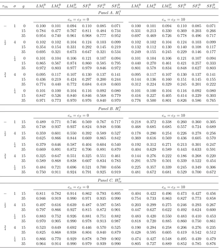
thus allowing for both upward and downward volatility shifts, with the chosen magnitudes being substantial for illustrative purposes. The other simulation DGP settings are as in Figures 3 and 4, however for brevity we now only consider a subset of the values for g given by g

= _f0;15;35_g. The results are shown in Tables 1 (a) and (b); these include the previously-considered homoskedastic case (obtained by setting = 1) as a benchmark for sizes and powers (note that in the tables, SupF is abbreviated to SF). Table 1 (a) considers the stochastic parameter variation of HS_{, while Table 1 (b) considers the non-stochastic parameter variation}

ofHN. Size results are reported only in Panel A of Table 1 (a), to avoid unnecessary duplication. In Panel A of Table 1 (a) the alternative is H₁S (intercept variation). Beginning with empirical sizes of our procedures (g = 0), we see that heteroskedasticity has only a modest e¤ect when compared to the benchmark homoskedastic case (particularly for the LM-based procedures). This suggests that the wild bootstrap is performing reasonably well in reproducing the patterns of heteroskedasticity present. Turning to …nite sample power, in general terms we see that the upward volatility shift considered signi…cantly decreases powers relative to the benchmark homoskedastic powers, while the downward shift considered has the opposite e¤ect. These e¤ects are observed for both volatility break timings considered. An examination of the power levels between the procedures reveals that under heteroskedasticity, the patterns of relative powers are generally similar to those observed in the homoskedastic case. For an alternative of HS

x (slope parameter variation), from Panel B it appears that both upward and 6_{We also ran simulations forT= 200. These results were little di¤erent from those discussed here forT = 100}

downward volatility shifts can lead to a decrease in power when compared to the homoskedastic benchmark (although this e¤ect is rather small for the downward shift). The patterns of relative power levels between the procedures again largely mimic what we see under homoskedasticity. As might be expected, under the alternative H₁S_x (intercept and slope parameter variation), Panel C shows that the e¤ect of a volatility shift on test power involves a mixture of the e¤ects seen under H₁S and H_xS. In very general terms, the volatility e¤ect on LMB₁ andSupFB₁ under

HS

1x is most similar to that for H1S, the impact on LMBx and SupFBx under H1Sx is closer to

that for H_xS, while the e¤ect of the volatility shift on LMB_1x and SupFB_1x for H₁S_x is a hybrid of the e¤ects seen under H₁S and H_xS. In Table 1 (b), where the alternatives are H₁N, H_xN

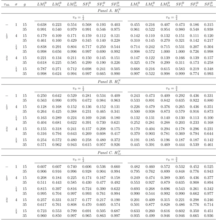
and H₁N_x, volatility shifts are seen to have qualitatively similar e¤ects on power, relative to the homoskedastic case, to those seen in Table 1 (a) forH₁S,H_xS andH₁S_x, respectively.

8

An Empirical Application

To illustrate how our proposed instability test procedures may be used in practice, we apply them to the U.S. annual equity series analysed in Welch and Goyal (2008), which is updated to cover the period 1926-2015 (T = 90) and is available at http://www.hec.unil.ch/agoyal/. Our yt variables are Rt, the log of the total return (including dividends) on the S&P 500 stock market index from year t 1 to t, and EPt, the equity premium, which subtracts the

corresponding risk-free rate (the Treasury Bill rate) fromRt. Thextpredictor variables (in each

case included in the bivariate PR with a one-period lag) are: the dividend yield, DYt, de…ned as the di¤erence between the log of dividends and the log of one-period lagged prices; the dividend payout ratio, DEt, de…ned as the di¤erence between the log of dividends and the log of earnings; and the long term rate of returns, LT Rt, the long term rate on government bonds.

While 1926-2015 represents the full sample period, we also consider the sub-sample 1926-2007, which pre-dates the global …nancial crisis, allowing analysis of any potential di¤erences when excluding the more recent years of instability.

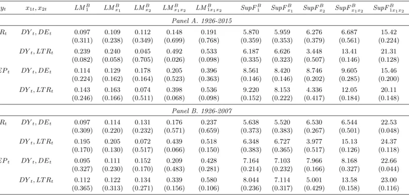
The results are shown in Table 2(a). The main entries are the computed values of the LMB₁,LMB_x,LMB_1x,SupFB₁,SupFB_x and SupFB_1x statistics. For theLM-based procedures, the number of lagged di¤erence terms in xtadded to the …tted regression (7) is determined using BIC selection starting from a maximum value of6. The same number of lagged di¤erence terms is employed for the SupF-based procedures in the …tted regression (10).

The entries in parentheses in the column labelled xt are bootstrap p-values for a standard KPSS statistic applied to each predictor (with the long run variance estimate based on the quadratic spectral kernel with automatic bandwidth selection), obtained using the wild boot-strap method of Cavaliere and Taylor (2005) with499bootstrap replications. Thesep-values are small in all cases, implying rejection of the null of stationarity against the unit root alternative for each series. As is well known, the KPSS test also rejects stationarity with high probability when the series under test displays local-to-unit root behaviour, so at the very least these results are indicative of a high degree of persistence being present in each of the predictor series.

The entries in parentheses underneath the main entries are the bootstrap p-values for the LMB₁,LMB_x,LMB_1x,SupFB₁,SupFB_x andSupFB_1xstatistics, based onB= 499bootstrap replica-tions. Considering …rst the results for the full sample period 1926-2015, strong evidence against

H0 being true is provided by theLMB1 andLMBx tests statistics for theRt-DYtpairing, and, to

a lesser extent, for theEPt-DYtpairing viaLMB_x. No evidence againstH0 is seen (i.e. no

rejec-tion at convenrejec-tional signi…cance levels) for theDEtand LT Rtpredictors, regardless of whether Rt orEPt is employed. Turning to the pre-crisis sub-sample, evidence againstH0 is again seen

for Rt-DYt (now also including SupFB_1x at the 0.10-level). Some evidence is also found again for EPt-DYt, this time via the SupFB1x test rather than the LMBx test. The change of sample

period has no e¤ect on the lack of rejections when using theDEt and LT Rt predictors. Table 2(a) also reports, under _jIV_j, the absolute value of the heteroskedasticity-robust IV

t-test of Breitung and Demetrescu (2015) for predictability ofytbyxt 1. This statistic combines

fractional and sine function instruments and tests the signi…cance of the estimated coe¢ cient on xt 1, having a standard normal limit distribution under the null of no predictability. Its

p-value is reported in parentheses. According to _jIV_j, there is strong evidence of predictability in both the Rt-LT Rt and EPt-LT Rt relationships when the 1926-2007 sub-sample is

consid-ered. Interestingly, neither of these pairings were found to be subject to parameter instability according to our battery of bootstrap procedures.

To informally examine the extent to which parameter instability appears present in these PRs, Figure 5 plots rolling window IV coe¢ cient estimates and approximate 0.10-level standard error bounds. These are based on a rolling window length set at_b0:25T_c observations, and the

x-axis dates correspond to the end of a given window sub-sample. Although it is di¢ cult to make any …rm conclusions, on examining Figure 5, we might be led to tentatively conclude that the most pronounced parameter variation is associated with the Rt-DYt and EPt-DYtpairings (Figures 5(a) and 5(d)). This would be in line with our bootstrap test outcomes in Table 2(a). Also, it is credible to consider that the least pronounced parameter variation observed is associated with Rt-DEt and EPt-DEt (Figures 5(b) and 5(e)), which would tie in with the generally largep-values for the associated instability tests. The estimated parameter values are also generally fairly close to zero, which is in line with _jIV_j in Table 2(a) …nding no evidence of predictability. The parameter estimates for Rt-LT Rt and EPt-LT Rt (Figures 5(c) and 5(f))

display relative constancy at positive values over much of the sample period, which is compatible with our instability tests not rejecting, yet at the same time_jIV_jindicating predictability for the earlier sub-sample. That the rolling parameter estimates reduce to insigni…cant levels towards the end of the full sample period could explain why_jIV_jdoes not reject for the full sample; on the other hand, it appears from the instability test results that this change is not substantial enough, in either magnitude or duration, to be detected by our test procedures.

In Table 2(b) we consider instability tests allowing for multiple predictors, using two predic-tors together by combiningDYt, the predictor for which most evidence of instability was found,