Majority-Inverter Graph: A New Paradigm for Logic Optimization

(1)

Majority-Inverter Graph: A New Paradigm for

Logic Optimization

Luca Amar´u,

Student Member, IEEE

, Pierre-Emmanuel Gaillardon,

Member, IEEE

,

Giovanni De Micheli,

Fellow, IEEE

Abstract— In this paper, we propose a paradigm shift in representing and optimizing logic by using only majority (MAJ) and inversion (INV) functions as basic operations. We represent logic functions by Majority-Inverter Graph (MIG): a directed acyclic graph consisting of three-input majority nodes and regu-lar/complemented edges. We optimize MIGs via a new Boolean algebra, based exclusively on majority and inversion operations, that we formally axiomatize in this work. As a complement to MIG algebraic optimization, we develop powerful Boolean methods exploiting global properties of MIGs, such as bit-error masking. MIG algebraic and Boolean methods together attain very high optimization quality. Considering the set of IWLS’05 benchmarks, our MIG optimizer (MIGhty) enables a 7% depth reduction in LUT-6 circuits mapped by ABC while also reducing size and power activity, with respect to similar AIG optimization. Focusing on arithmetic intensive benchmarks instead, MIGhty enables a 16% depth reduction in LUT-6 circuits mapped by ABC, again with respect to similar AIG optimization. Employed as front-end to a delay-critical 22-nm ASIC flow (logic synthesis + physical design)MIGhtyreduces the average delay/area/power by 13%/4%/3%, respectively, over 31 academic and industrial benchmarks. We also demonstrate delay/area/power improve-ments by 10%/10%/5% for a commercial FPGA flow.

Index Terms— Design methods and tools, Optimization, Ma-jority Logic, Boolean Algebra, DAG, Logic Synthesis.

I. INTRODUCTION

N

OWADAYS,Electronic Design Automation(EDA) tools are challenged by design goals at the frontier of what is achievable in advanced technologies. In this scenario, extend-ing the optimization capabilities of logic synthesis tools is of paramount importance.

In this paper, we propose a paradigm shift in representing and optimizing logic, by using only majority (MAJ) and inversion (INV) as basic operations. We use the terms in-version and complementation interchangeably. We focus on majority functions because they lie at the core of Boolean function classification [1]. Thanks to that, majority inher-its the expressive power from many other function classes. Together with inversion, majority can express all Boolean functions. Based on these primitives, we present in this work the Majority-Inverter Graph (MIG), a logic representation structure consisting of three-input majority nodes and regu-lar/complemented edges. MIGs include anyAND/OR/Inverter Graphs (AOIGs), containing also the popular AIGs [2]. To provide native manipulation of MIGs, we introduce a novel Boolean algebra, based exclusively on majority and inversion operations [3]. We define a set of five transformations forming a sound and complete axiomatic system. Using a sequence of these primitive axioms, it is possible to manipulate ef-ficiently a MIG and reach all points in the representation

The authors are with the Integrated Systems Laboratory, Swiss Federal In-stitute of Technology, Lausanne, EPFL, 1015 Lausanne, Switzerland (e-mail: [email protected]). Copyright (c) 2015 IEEE. Personal use of this material is permitted. However, permission to use this material for any other purposes must be obtained from the IEEE by sending an email to [email protected].

space. We apply MIG algebra axioms locally, to design fast and efficient MIG algebraic optimization methods. We also exploit global properties of MIGs to design slower but very effective MIG Boolean optimization methods [4]. Specifically, we take advantage of the error masking property of majority operators. By selectively inserting logic errors in a MIG, successively masked by majority nodes, we enable strong simplifications in logic networks. MIG algebraic and Boolean methods together attain very high optimization quality. For example when targeting depth reduction, our MIG optimizer, MIGhty, transforms a ripple carry structure into a carry look-ahead like one. Considering the set of IWLS’05 benchmarks, MIGhty enables a 7% depth reduction in LUT-6 circuits mapped by ABC [2] while also reducing size and power activity, with respect to similar AIG optimization. Focusing on arithmetic intensive benchmarks,MIGhtyenables a 16% depth reduction in LUT-6 circuits, again with respect to similar AIG optimization. Employed as front-end to a delay-critical 22-nm ASIC flow MIGhty reduces the average delay/area/power by 13%/4%/3%, respectively, over academic and industrial benchmarks, as compared to a leading commercial ASIC flow. We demonstrate improvements in delay/area/power metrics by 10%/10%/5% for a commercial 28-nm FPGA flow.

The remainder of this paper is organized as follows. Section II gives background on logic representation and optimization. Section III presents MIGs with their properties and associ-ated Boolean algebra. Section IV proposes MIG algebraic optimization methods and Section V describes MIG Boolean optimization methods. Section VI shows experimental results for MIG-based optimization and compares them to the state-of-the-art academic tools. Section VI also shows results for MIG-based optimization employed as front-end to commercial ASIC and FPGA design flows. Section VII is a conclusion.

II. BACKGROUND ANDMOTIVATION

This section presents first a background on logic represen-tation and optimization for logic synthesis. Then, it introduces the necessary notations and definitions for this work.

A. Logic Representation

The (efficient) way logic functions are represented in EDA tools is key to design efficient hardware. On the one hand, logic representations aim at having the fewest number of primitive elements (literals, sum-of-product terms, nodes in a logic network, etc.) in order to (i) have small memory footprint and (ii) be covered by as few library elements as possible. On the other hand, logic representation forms must be simple enough to manipulate. This may require having a larger number of primitive elements but with simpler manipulation laws. The choice of a computer data-structure is a trade-off between compactness and manipulation easiness.

(2)

In the early days of EDA, the standard representation form for logic was the Sum Of Product (SOP) form, i.e., a dis-junction (OR) of conjuctions (AND) made of literals [5]. This standard was driven by PLA technology whose functionality is naturally modeled by a SOP [6]. Other two-level forms, such as product-of-sums or EX-SOP, have been studied at that time [17]. Two-level logic is compact for small sized functions but, beyond that size, it becomes too large to be efficiently mapped into silicon. Yet, two-level logic has been supported by efficient heuristic and exact optimization algorithms. With the advent of VLSI, the standard representation for logic moved from SOP to Directed Acyclic Graphs(DAGs) [7]. In a DAG-based logic representation, nodes correspond to logic functions (gates) and directed edges (wires) connect the nodes. Nodes’ functions can be internally represented by SOPs lever-aging the proven efficiency of two-level optimization. From a global perspective, general optimization procedures run on the entire DAG. While being potentially very compact, DAGs without bounds on the nodes’ functionality are not easy to optimize. This is because this kind of representation demands that optimization techniques deal with all possible types and sizes of functions which is impractical. On top of that, the cumulative memory footprint for eachfunctionally unbounded node is potentially very large. Restricting the permissible node function types alleviates this issue. At the extreme case, one can focus on just one type of function per node and add complemented/regular attributes to the edges. Even though in principle, this restriction increases the representation size, in practice it unlocks better (smaller) representations because it supports more effective logic optimization simplifying a DAG. A notable example of DAG where all the nodes realize the same function is Binary Decision Diagrams (BDDs) [11]. In BDDs, nodes act as 2:1 multiplexers. With additional restric-tion on the ordering of input variables, BDDs are canonical and provide very efficient manipulation procedures. For this reason, BDDs found application in various areas of EDA, such as verification, testing, optimization, automated reasoning, etc [5]. However, the price for such an optimal manipulation efficiency is the BDD size, which is often too large for direct mapping into silicon. Even though BDDs are not usually mapped directly into silicon, they support in various ways logic manipulation tasks in some optimization algorithms [9]. Another DAG where all nodes realize the same function is the And-Inverter Graph (AIG) [2], [10] where nodes act as two-input ANDs. AIGs can be optimized through traditional Boolean algebra axioms and derived theorems. Iterated over the whole AIG, local transformations produce very effective results and scale well with the size of the circuits. This means that, overall, AIGs can be made remarkably small through logic optimization. For this reason, AIG is one of the current representation standards for logic synthesis.

B. Logic Optimization

Logic optimization consists of manipulating a logic rep-resentation structure in order to minimize some target metric. Usual optimization targets are size (number of nodes/elements), depth (maximum number of levels), inter-connections (number of edges/nets), etc.

Logic optimization methods are closely coupled to the data structures they run on. In two-level logic representation (SOP), optimization aims at reducing the number of terms.

ESPRESSO is the main optimization tool for SOP [6]. Its algorithms operate on SOP cubes and manipulate the ON-, OFF- and DC-covers iteratively. In its default settingsON-, ESPRESSO uses fast heuristics and does not guarantee to reach the global optimum. However, an exact optimization of two level logic is available (under the name of ESPRESSO-exact) and often run in a reasonable time. The exact two-level optimization is based on Quine-McCluskey algorithm [18]. Moving to DAG logic representation (also called multi-level logic), optimization aims at reducing graph size and depth or other accepted complexity metrics. There, DAG-based logic optimization methods are divided into two groups: Algebraic methods, which are fast and Boolean methods, which are slower but may achieve better results [21]. Traditional al-gebraic methods assume that DAG nodes are represented in SOP form and treat them as polynomials [7], [19]. Algebraic operations are selectively iterated over all DAG nodes, until no improvement is possible. Basic algebraic operations are extraction, decomposition, factoring, balancing and substitu-tion [20], [21]. Their efficient runtime is enabled by theories of weak-division and kernel extraction. In contrast, Boolean methods do not treat the functions as polynomials but handle their true Boolean nature using Boolean identities as well as (global) don’t cares (circuit flexibilities) to get a better solution [5], [21], [24]–[26]. Boolean division and substi-tution techniques trade off runtime for better minimization quality. Functional decomposition is another Boolean method which aims at representing the original function by means of simpler component functions. The first attempts at functional decomposition [27]–[29] make use of decomposition charts to find the best component functions. Since the decomposition charts grow exponentially with the number of variables these techniques are only applicable to small functions. A different, and more scalable, approach to functional decomposition is based on the BDD data structure. A particular class of BDD nodes, called dominator nodes, highlights advantageous func-tional decomposition points [9]. BDD decomposition can be applied recursively and is capable of exploiting optimization opportunities not visible by algebraic counterparts [9], [22], [23]. Recently, disjoint support decomposition has also been considered to optimize locally small functions and speedup logic manipulation [30], [31]. It is worth mentioning that the main difficulty in developing Boolean algorithms is due to the unrestricted space of choices. This makes more difficult to take good decisions during functional decomposition.

Advanced DAG optimization methodologies, and associated tools, use both algebraic and Boolean methods. When DAG nodes are restricted to just one function type the optimization procedure can be made much more effective. This is because logic transformations are designed specifically to target the functionality of the chosen node. For example, in AIGs, logic transformations such as balancing, refactoring, and general rewriting are very effective. For example, balancing is based on the associativity axiom from traditional Boolean algebra [12], [13]. Refactoring operates on an AIG subgraph which is first collapsed into SOP and then factored out [19]. General rewriting conceptually includes balancing and refactoring. Its purpose is to replace AIG subgraphs with equivalent pre-computed AIG implementations that improve the number of nodes and levels [12]. By applying local, but powerful, transformations many times during AIG optimization it is

(3)

possible to obtain very good result quality. The restriction to AIGs makes it easier to assess the intermediate quality and to develop the algorithms, but in general is more prone to local minimum. Nevertheless, Boolean methods can still complement AIG optimization to attain higher quality of results [2], [24].

In this work, we present a new representation form, based on majority and inversion, with its native Boolean algebra. We show algebraic and Boolean optimization techniques for this data structure unlocking new points in the design space.

Note that early attempts to majority logic have already been reported in the 60’s [14]–[16], but, due to their inherent complexity, failed to gain momentum later on in automated synthesis. We address, in this paper, the unique opportunity led by majority logic in a contemporary synthesis flow. C. Notations and Definitions

We provide hereafter notations and definitions on Boolean algebra and logic networks.

1) Boolean Algebra: In the binary Boolean domain, the symbolBindicates the set of binary values{0,1}, the symbols ∧ and ∨ represent the conjunction (AND) and disjunction (OR) operators, the symbol 0 represents the complementation (INV) operator and 0/1 are the false/true logic values. Alter-native symbols for ∧ and ∨ are · and +, respectively. The standard Boolean algebra (originally axiomatized by Hunting-ton [32]) is a non-empty set(_B,∧,∨,0,0,1)subject toidentity, commutativity, distributivity, associativityandcomplement ax-ioms over ∧,∨ and 0 [1]. For the sake of completeness, we report these basic axioms in Eq. 1. Such axioms will be used later on in this work for proving theorems.

This axiomatization for Boolean algebra is sound and complete [33]. Informally, it means that logic arguments, or formulas, proved by axioms in∆are valid (soundness) and all true logic arguments are provable (completeness). We refer the reader to [33] for a more formal discussion on mathematical logic. In practical EDA applications, only sound and complete axiomatizations are of interest.

Other Boolean algebras exist, with different operators and axiomatizations, such as Robbins algebra, Freges algebra, Nicods algebra, etc. [33]. Boolean algebras are the basis to operate on logic networks.

∆

                                             Identity : ∆.I x∨0 =x x∧1 =x Commutativity :∆.C x∧y=y∧x x∨y=y∨x Distributivity : ∆.D x∨(y∧z) = (x∨y)∧(x∨z) x∧(y∨z) = (x∧y)∨(x∧z) Associativity :∆.A x∧(y∧z) = (x∧y)∧z x∨(y∨z) = (x∨y)∨z Complement :∆.Co x∨x0= 1 x∧x0= 0 (1)

2) Logic Network: A logic network is a Directed Acyclic Graph(DAG) with nodes corresponding to logic functions and directed edges representing interconnection between the nodes.

The direction of the edges follows the natural computation from inputs to outputs. The terms logic network, Boolean net-work, and logic circuit are used interchangeably in this paper. A logic network is saidirredundantif no node can be removed without altering the Boolean function that it represents. A logic network is saidhomogeneousif each node represents the same logic function and has a fixed indegree, i.e., the number of incoming edges or fan-in. In a homogeneous logic network, edges can have a regular or complemented attribute. The depth of a node is the length of the longest path from any primary input variable to the node. The depth of a logic network is the largest depth among all the nodes. The size of a logic network is the number of its nodes.

3) Self-Dual Function: A logic functionf(x, y, .., z)is said to beself-dualiff =f0(x0, y0, .., z0)[1]. By complementation, an equivalentself-dual formulation isf0 =f(x0, y0, .., z0).

4) Majority Function: Then-input (nbeing odd) majority function M returns the logic value assumed by more than half of the inputs [1]. For example, the three input majority function M(x, y, z) is represented in terms of ∧,∨ by (x∧

y)∨(x∧z)∨(y∧z). Also(x∨y)∧(x∨z)∧(y∨z)is a valid representation for M(x, y, z). The majority function is self-dual[1].

III. MAJORITY-INVERTERGRAPHS

In this section, we present MIGs and their representation properties. Then, we show a new Boolean algebra natively fitting the MIG data structure. Finally, we discuss the error masking capabilities of MIGs from an optimization standpoint. A. MIG Logic Representation

Definition 3.1: An MIG is a homogeneous logic network with an indegree equal to 3 and each node representing the majority function. In a MIG, edges are marked by a regular or complemented attribute.

To determine some basic representation properties of MIGs, we compare them to the well-knownAND/OR/Inverter Graphs (AOIGs) (which include AIGs). In terms of representation expressiveness, the elementary bricks in MIGs are majority operatorswhile in AOIGs there are conjunctions (AND) and disjunctions (OR). It is worth noticing that a majority operator M(x, y, z) behaves as the conjunction operator AN D(x, y)

when z = 0 and as the disjunction operator OR(x, y) when z = 1. Therefore, majority is actually a generalization of both conjunction and disjunction. Recall that M(x, y, z) =

xy+xz+yz. This property leads to the following theorem. Theorem 3.1: MIGs⊃AOIGs.

Proof:In both AOIGs and MIGs, inverters are represented by complemented edge markers. An AOIG node is always a special case of a MIG node, with the third input biased to logic 0 or 1 to realize an AND or OR, respectively. On the other hand, a MIG node is never a special case of an AOIG node, because the functionality of the three input majority cannot be realized by a unique AND or OR.

As a consequence of the previous theorem, MIGs are at least as good as AOIGs but potentially much better, in terms of representation compactness. Indeed, in the worst case, one can replace node-wise AND/ORs by majorities with the third input biased to a constant (0/1). However, even a more compact MIG

(4)

representation can be obtained by fully exploiting its node functionality rather than fixing one input to a logic constant.

Fig. 1 depicts a MIG representation example for f =

x3·(x2+ (x01+x0)0). The starting point is a traditional AOIG.

Such AOIG has 3 nodes and 3 levels of depth, which is the best representation possible using just AND/ORs. The first MIG is obtained by a one-to-one replacement of AOIG nodes by MIG nodes. As shown by Fig. 1, a better MIG representation is possible by taking advantage of the majority function. This transformation will be detailed in the rest of this paper. In this way, one level of depth is saved with the same node count.

AOIG%!%MIG% AND% OR% OR% x0% x1% x3% x2% f% MAJ% MAJ% MAJ% x0% x1% x3% x2% f% 1% 1% 1% MAJ% MAJ% f% MAJ% x3% 1% 1% x2% x3% x0% x1% MIG%!%MIGopt%

Fig. 1: MIG representation for f = x3·(x2+ (x01+x0)0).

Complementation is represented by bubbles on the edges. MIGs inherit from AOIGs some important properties, like universality and AIG inclusion. This is formalized by the following.

Corollary 3.2: MIGs⊃AIGs.

Proof: MIGs⊃AOIGs ⊃AIGs =⇒ MIGs⊃AIGs Corollary 3.3: MIG is an universal representation form.

Proof: MIGs⊃AOIGs ⊃AIGs that are universal repre-sentation forms [10].

So far, we have shown that MIGs extend the representation capabilities of AOIGs. However, we need a proper set of manipulation tools to handle MIGs and automatically reach compact representations. For this purpose, we introduce here-after a new Boolean algebra, based on MIG primitives. B. MIG Boolean Algebra

We present a novel Boolean algebra, defined over the set

(B, M,0,0,1), where M is the majority operator of three variables and0 is the complementation operator. The following five primitive transformation rules, referred to as Ω, form an axiomatic systemfor(_B, M,0,0,1). All variables belong toB.

Ω

                               Commutativity :Ω.C M(x, y, z) =M(y, x, z) =M(z, y, x) Majority :Ω.M if(x=y):M(x, x, z) =M(y, y, z) =x=y if(x=y0): M(x, x0, z) =z Associativity :Ω.A M(x, u, M(y, u, z)) =M(z, u, M(y, u, x)) Distributivity : Ω.D M(x, y, M(u, v, z)) =M(M(x, y, u), M(x, y, v), z) Inverter Propagation : Ω.I M0(x, y, z) =M(x0, y0, z0) (2) AxiomΩ.C defines a commutativity property. AxiomΩ.M declares a 2 over 3 decision threshold. Axiom Ω.A is an associative law extended to ternary operators. Axiom Ω.D establishes a distributive relation over majority operators. Axiom Ω.I expresses the interaction between M and com-plementation operators. It is worth noticing that Ω.I does not

require operation type change like De Morgan laws, as it is well known from self-duality [1].

We prove that(B, M,0,0,1)axiomatized byΩis an actual Boolean algebra by showing that it induces a complemented distributive lattice [34].

Theorem 3.4: The set(_B, M,0_,₀_,₁₎_{subject to axioms in}_Ω

is a Boolean algebra.

Proof:The systemΩembed median algebra axioms [35]. In such scheme,M(0, x,1) =xfollows from Ω.M. In [36], it is proved that a median algebra with elements 0 and 1

satisfyingM(0, x,1) =xis a distributive lattice. Moreover, in our scenario, complementation is well defined and propagates through the operator M (Ω.I). Combined with the previous property on distributivity, this makes our system a comple-mented distributive lattice. Every complecomple-mented distributive lattice is a Boolean algebra [34].

Note that there are other possible axiomatic systems for

(B, M,0,0,1). For example, one can show that in the presence ofΩ.C,Ω.AandΩ.M, the rule inΩ.Dis redundant [37]. In this work, we consider Ω.D as part of the axiomatic system for the sake of simplicity.

1) Derived Theorems: Several other complex rules, for-mally called theorems, in (B, M,0,0,1) are derivable from Ω. Among the ones we encountered, three rules derived from

Ω are of particular interest to logic optimization. We refer to them as Ψ and are described hereafter. In the following, the symbol zx/y represents a replacement operation, i.e., it

replacesxwithy in all its appearence inz.

Ψ

                 Relevance – Ψ.R M(x, y, z) =M(x, y, zx/y0) Complementary Associativity –Ψ.C M(x, u, M(y, u0, z)) =M(x, u, M(y, x, z)) Substitution – Ψ.S M(x, y, z) = M(v, M(v0_{, M} v/u(x, y, z), u), M(v0, Mv/u0(x, y, z), u0)) (3) The first rule, relevance(Ψ.R), replaces reconvergent vari-ables with their neighbors. For example, consider the func-tion f = M(x, y, M(w, z0, M(x, y, z))). Variables x and y are reconvergent because they appear in both the bot-tom and the top majority operators. In this case, relevance

(Ψ.R) replaces x with y0 in the bottom majority as f =

M(x, y, M(w, z0, M(y0, y, z))). This representation can be further reduced tof =M(x, y, w)by usingΩ.M.

The second rule, complementary associativity(Ψ.C), deals with variables appearing in both polarities. Its rule of re-placement is M(x, u, M(y, u0, z)) = M(x, u, M(y, x, z)) as depicted by Eq. 3.

The third rule, substitution(Ψ.S), extends variable replace-ment to the non-reconvergent case. We refer the reader to Fig. 2 for an example about substitution(Ψ.S)applied to a 3-input parity function.

Hereafter, we show howΨrules can be derived from Ω. Theorem 3.5: Ψrules are derivable byΩ.

Proof:Relevance (Ψ.R): LetS be the set of all possible input patterns forM(x, y, z). LetSx=y (Sx=y0) be the subset of S such that x = y (x = y0) condition is true. Note that Sx=y∩Sx=y0 =∅andS_x₌_y∪S_x₌_y0 =S. According toΩ.M, variablez inM(x, y, z)is only relevant forSx=y0. Thus, it is

(5)

possible to replacexwithy0, i.e., (x/y0), in all its appearance inz, preserving the original functionality.

Complementary Associativity (Ψ.C):

M(x, u, M(u0, y, z)) =M(M(x, u, u0), M(x, u, y), z)(Ω.D) M(M(x, u, u0), M(x, u, y), z) =M(x, z, M(x, u, y))(Ω.M) M(x, z, M(x, u, y)) =M(x, u, M(y, x, z))(Ω.A)

Substitution (Ψ.S): We setM(x, y, z) =kfor brevity. k=M(v, v0, k) =(Ω.M)

M(M(u, u0, v), v0, k) =(Ω.M)

M(M(v0, k, u), M(v0, k, u0), v) =(Ω.D) Then, M(v0, k, u) =M(v0, kv/u, u)(Ψ.R)

andM(v0, k, u0) =M(v0, kv/u0, u)(Ψ.R)

Recalling thatk=M(x, y, z), we finally obtain:M(x, y, z) =

M(v, M(v0, Mv/u(x, y, z), u), M(v0, Mv/u0(x, y, z), u0)) 2) Soundness and Completness: The set (B, M,0,0,1) to-gether with axiomsΩand derivable theorems form our major-ity logic system. In a computer implementation of our majormajor-ity logic system, the natural data structure for (_B, M,0,0,1) is a MIG and the associated manipulation tools are Ω and Ψ

transformations. In order to be useful in practical applications, such as EDA, our majority logic system needs to satisfy fundamental mathematical properties such as soundness and completeness [33]. Soundness means that every argument provable by the axioms in the system is valid. This guarantees preserving of correctness. Completeness means that every valid argument has a proof in the system. This guarantees uni-versal logic reachability. We show that our majority Boolean algebra is sound and complete.

Theorem 3.6: The Boolean algebra (B, M,0,0,1) axioma-tized by Ωis sound and complete.

Proof: We first consider soundness. Here, we need to prove that all axioms in Ω are valid, i.e., preserve the true behavior (correctness) of a system. Rules Ω.C andΩ.M are valid because they express basic properties (commutativity and majority decision rule) of the majority operator. Rule Ω.I is valid because it derives from the self-duality of the majority operator. For rules Ω.D and Ω.A, a simple way to prove their validity is to build the corresponding truth tables and check that they are actually the same. It is an easy exercise to verify that it is true. We consider now completeness. Here, we need to prove that every valid argument, i.e., (_B, M,0_,₀_,₁₎

-formula, has a proof in the system Ω. By contradiction, suppose that a true (_B, M,0_,₀_,₁₎_{-formula, say} _α_{, cannot be}

proven true using Ω rules. Such (B, M,0,0,1)-formula α can always be reduced by Ψ.S rules into a (_B,∧,∨,0_,₀_,₁₎

-formula. This is because Ψ.S can behave as Shannon’s ex-pansion by setting v = 1anduto a logic variable. Using ∆

(Eq. 1), all(B,∧,∨,0,0,1)-formulas can be proven, including

α. However, every (_B,∧,∨,0_,₀_,₁₎_{-formula is also contained}

by (B, M,0,0,1), where ∧ and ∨ are emulated by majority operators. Moreover, rules inΩwith one input fixed to0and1

behaves as∆rules (Eq. 1). This means that alsoΩis capable to prove the reduced (_B, M,0_,₀_,₁₎_-formula _α_{, contradicting}

our assumption. Thus our system is sound and complete. As a corollary of Ωsoundness, all rules in Ψare valid. Corollary 3.7: Ψrules are valid in(B, M,0,0,1).

Proof: Ψ rules are derivable by Ω as shown in Theo-rem 3.5. Then, Ωrules are sound in (B, M,0,0,1) as shown

in Theorem 3.6. Rules derivable from sound axioms are valid in the original domain.

As a corollary of Ω completeness, any element of a pair of equivalent (B, M,0,0,1)-formulas, or MIGs, can be trans-formed one into the other by a sequence ofΩtransformations. From now on, we use MIGs to refer to functions in the

(_B, M,0,0,1) domain. Still, the same arguments are valid for

(B, M,0,0,1)-formulas.

Corollary 3.8: It is possible to transform any MIGαinto any other logically equivalent MIG β, by a sequence of transformations inΩ.

Proof: MIGs are defined over the (B, M,0,0,1) do-main. Following from Theorem 3.6, all valid arguments over

(B, M,0,0,1)can be proved by a sequence ofΩrules. A valid argument is then M(1, M(α, β0,0), M(α0, β,0)) = 0 which reads ”α is never different from β” according to the initial hypothesis. It follows that the sequence of Ω rules proving such argument is also logically transformingαinto β.

3) Reachability: To measure the efficiency of a logic sys-tem, thus of its Boolean algebra, one can study (i) the ability to perform a desired task and (ii) the number of basic operations required to perform such a task. In the context of this work, the task we care about is logic optimization. For the graph size and graph depth metrics, MIGs can be smaller than AOIGs because of Theorem 3.1. However, the complexity of Ω sequences required to reach those desirable MIGs is not obvious. In this regard, we give an insight about the majority logic system efficiency by comparing the number ofΩrules needed to get an optimized MIGs with the number of ∆ rules needed to get an evenly optimized AIGs. This type of efficiency metric is often referred to as reachability, i.e., the ability to reach a desired representation form with the smallest number of steps possible.

Theorem 3.9: For a given optimization goal and an initial AOIG, the number ofΩrules needed to reach this goal with a MIG is smaller, or at most equal, than the number of∆rules needed to reach the same goal with an AOIG.

Proof:Consider the shortest sequence of∆rules meeting the optimization goal with an AOIG. On the MIG side, assume to start with the initial AOIG replacing node-wise AND/OR nodes with pre-configured majority nodes. Note that Ωrules with one input fixed to0/1behave as∆rules. So, it is possible to emulate the same shortest sequence of ∆ rules in AOIGs withΩin MIGs. This is just an upper bound on the shortest sequence ofΩrules. Exploiting the full Ωexpresiveness and MIG compactness, this sequence can be further shortened.

For a deeper theoretical study on majority logic expresive-ness, we refer the reader to [38]. In this work, we use the mathematical theory presented so far to define a consistent logic optimization framework. Then, we give experimental evidence on the benefits predicted by the theory. Results in Section VI show indeed a depth reduction, over the state-of-the-art techniques, up to48×thanks to our majority logic sys-tem. More details on the experiments are given in Section VI. Operating on MIGs via the new Boolean algebra is one nat-ural approach to run logic optimization. Interestingly enough, other approaches are also possible. In the following, we show how MIGs can be optimized exploiting other properties of the majority operator, such as bit-error masking.

(6)

C. Inserting Safe Errors in MIG

MIGs are hierarchical majority voting systems. One notable property of majority voting is the ability to correct different types of bit-errors. This feature is inherited by MIGs, where the error masking property can be exploited for logic optimiza-tion. The idea is to purposely introduce logic errors that are succesively masked by the voting resilience in MIG nodes. If such errors are advantageous, in terms of logic simplifications, better MIG representations can be generated.

In the immediate following, we briefly review hereafter notations and definitions on logic errors [5], [39]. Then, we present the theoretical grounds for “safe error insertion” in MIGs. We define what type of errors, and at what overhead cost, can be introduced. Note that, in this work, we use the worderroneousto highlight the presence of a logic error. Our notation do not relate to testing or other fields.

Definition The logic error in function f is defined as the difference between f and its erroneous version g and is computed asf ⊕g.

In principle, a logic error can be determined for any two circuits. In practical cases, a logic error is interpreted as a perturbation Aon an original logic circuitf.

Notation A logic circuitf affected by errorAis writtenfA. For example, consider the functionf = (a+b)·c. An error A defined as ”fix variable b to0 ” (A:b = 0) leads here to fA₌_ac_{. In general, an error flips} _k_{entries in the truth table}

of the affected function. In the above example,k= 1. To insert safe (permissible) errors in a MIG we consider a node w and we triplicate the sub-trees rooted at it. In each version ofwwe introduce logic errors heavily simplifying the MIG. Then, we use the three erroneous versions ofwas inputs to a top majority node exploiting the error masking property. Unfortunately, a majority node cannot mask all types of errors. This limits our choice of permissible errors.Orthogonal errors, defined hereafter, fit our purposes. Informally, two logic errors are orthogonal if for any input pattern they cannot happen simultaneously. In the majority voting scenario the orthogonality is important because it guarantees that no two logic errors happen at the same time which would corrupt the original functionality.

Definition Two logic errorsAandB on a logic circuitf are said orthogonalif (fA_⊕_f₎_·₍_fB_⊕_f_{) = 0}_.

To give an example oforthogonalerrors consider again the function f = (a+b)·c. Here, the two errors A: a+b = 1 and B: c = 0 are actually orthogonal. Indeed, by logic simplification, we get(c⊕f)·(0⊕f) = (((a+b)c)0c+ ((a+

b)c)c0)·((a+b)c) = ((a+b)c)0c·((a+b)c) = 0. Instead, the errors A: a+b= 1 andB: c = 1 are notorthogonal for f. This is because the input(1,1,1) triggers both errors.

Now consider back a generic MIG rootw. LetA,B andC be three pairwise orthogonalerrors on w. Being all pairwise orthogonal, a top majority nodeM(wA_{, w}B_{, w}C₎ _{is capable}

to mask A, B and C orthogonal errors restoring the original functionality ofw. This is formalized in the following theorem. Theorem 3.10: Letw be a generic node in a MIG. LetA, B andC be three pairwiseorthogonal errors onw. Then the following equation holds: w=M(wA, wB, wC)

Proof: The equation w = M(wA_{, w}B_{, w}C₎ _is

log-ically equivalent to w ⊕ M(wA_{, w}B_{, w}C_{) = 0}_{. The} _⊕

(XOR) operator propagates into the majority operator as w⊕M(wA_{, w}B_{, w}C_{) =} _M₍_wA _⊕_{w, w}B _⊕_{w, w}C _⊕_w₎_.

Recalling that M(a, b, c) = ab +ac +bc we rewrite the previous expression as(wA_⊕_w₎_·₍_wB_⊕_w₎₊₍_wA_⊕_w₎_·₍_wC_⊕ w) + (wB ⊕w)·(wC ⊕w). As A, B and C are pairwise orthogonal, we have that each term is 0, so 0 + 0 + 0 = 0. So,w⊕M(wA, wB, wC) = 0.

Note that a MIGw=M(wA_{, w}B_{, w}C₎_{can have up to three}

times the size and one more level of depth as the originalw. This means that simplifications enabled by orthogonal errors A, B and C must be significant enough to compensate for such overhead. Note also that this approach resembles triple modular redundancy [40] and its approximate variants [41], but operates differently. Here, we exploit the error masking property in majority operators to enable logic simplifications rather than covering potential hardware failures. More details on how to identify advantageous orthogonal errors in MIGs will be given in Section V-A together with related Boolean optimization methods.

In the following sections, we present algorithms for alge-braic and Boolean optimization of MIGs.

IV. MIG ALGEBRAICOPTIMIZATION

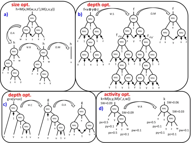
In this section, we propose algebraic optimization methods for MIGs. They exploit axioms and derived theorems of the novel Boolean algebra. Our algebraic optimization procedures target size, depth and switching activity reduction in MIGs. A. Size-Oriented MIG Algebraic Optimization

To optimize the size of a MIG, we aim at reducing the num-ber of its nodes. Node reduction can be done, at first instance, by applying the majority rule. In the MIG Boolean algebra domain this corresponds to the evaluation of the majority ax-iom (Ω.M) fromLeft to Right(L→R), asM(x, x, z) =x. A different node elimination opportunity arises from the distribu-tivity axiom (Ω.D), evaluated from Right to Left (R → L), as M(x, y, M(u, v, z)) = M(M(x, y, u), M(x, y, v), z). By applyingΩ.ML→RandΩ.DR→Lto all MIG nodes, in an

arbi-trary sequence, we can actually eliminate nodes. By repeating this procedure until no improvement exists, we designed a simple yet powerful procedure to reduce a MIG size. Embed-ding some intelligence in the graph exploration direction, e.g., the sequence of MIG nodes, immediately improves the opti-mization effectiveness. Note that the applicability of majority and distributivity depends on the particular MIG structure. Indeed, there may be MIGs where no direct node elimination is evident. This is because (i) the optimal size is reached or (ii) we are stuck in a local minimum. In the latter case, we want to reshape the MIG in order to encode new reduction opportunities. The rationale driving the reshaping process is to locally increase the number of common inputs/variables to MIG nodes. For this purpose, the associativity axioms (Ω.A,

Ψ.C) allow us to move variables between adjacent levels and the relevance axiom (Ψ.R) to exchange reconvergent variables. When a more radical transformation is beneficial, the substitution axiom (Ψ.S) replaces pairs of independent variables, temporarily inflating the MIG. Once the reshaping process has created new reduction opportunities, majority (Ω.ML→R) and distributivity (Ω.DR→L) are applied again

over the MIG to simplify it. The reshaping and elimination processes can be iterated over a user-defined number of cycles,

(7)

MAJ$ 1$ MAJ$ z$ 1$ MAJ$ 1$ z$ _MAJ$ 1$ MAJ$ y$ 1$ x$ MAJ$ 1$ y$ f=x!$!$y!$!$z!$ MAJ$ 1$ MAJ$ z$ 1$ MAJ$ 1$ z$ _MAJ$ 1$ MAJ$ y$ 1$ y$ MAJ$ 1$ y$ MAJ$ 1$ MAJ$ z$ 1$ MAJ$ 1$ MAJ$ 1$ MAJ$ y$ 1$ y$ MAJ$ 1$ MAJ$ x$ MAJ$ x$ MAJ$ x$ y$ f!$ f$_x\y!$ _f$_x\y’_!_$ MAJ$ MAJ$ f$ MAJ$ x$ y$ x$ z$ x$ z$ Ψ.S$ Ω.M$ MAJ$ MAJ$ w$ x$ x$ k=M(x,y,M(x’,z,w))$ y$ z$ Ψ.R$ _MAJ$ MAJ$ w$ x$ y$ k$ y$ z$ SW=0.09$ SW=0.09$ SW=0.03$ SW=0.06$ px=0.5$ py=0.1$ pw=0.1$ pz=0.1$ px=0.5$ px=0.5$ py=0.1$ pw=0.1$ pz=0.1$ py=0.1$ Ω.A$ MAJ$ MAJ$ MAJ$ v$ u$ x$ y$ g=x(y+uv)$ 1$ 1$ 1$ Ψ.C$ MAJ$ MAJ$ g$ MAJ$ x$ 1$ u$ v$ x$ y$ MAJ$ MAJ$ MAJ$ v$ u$ x$ y$ g$ 1$ x$ 1$ Ω.A$ Ω.M$ Ψ.R$ MAJ$ x$ MAJ$ y$ x$ z$ MAJ$ x$ w$ h=M(x,M(w,x,z’),M(z,x,y))$ MAJ$ x$ MAJ$ y$ x$ z$ MAJ$ x$ w$ z$ h$ MAJ$ x$ MAJ$ y$ x$ z$ MAJ$ x$ w$ x$ h$ h$ x$

depth&opt.&

size&opt.&

depth&opt.&

ac.vity&opt.&

a)&

b)&

c)&

d)&

Fig. 2: Examples of MIG optimization for size, depth and switching activity. calledeffort. Such MIG-size algebraic optimization strategy is

summarized in Alg. 1.

Algorithm 1 MIG Algebraic Size-Optimization Pseudocode INPUT:MIGα OUTPUT:Optimized MIGα.

for(cycles=0; cycles<effort; cycles++)do

Ω.ML→R(α); Ω.DR→L(α); Ω.A(α); Ψ.C(α); Ψ.R(α); Ψ.S(α); Ω.ML→R(α); Ω.DR→L(α); end for

reshape

eliminate

For the sake of clarity, we comment on the MIG-size algebraic optimization of a simple example, reported in Fig. 2(a). The input MIG is equivalent to the for-mula M(x, M(x, z0, w), M(x, y, z)), which has no evident simplification by majority and distributivity axioms. Con-sequently, the reshape process is invoked to locally in-crease the number of common inputs. Associativity Ω.A swaps w and M(x, y, z) in the original formula obtaining M(x, M(x, z0, M(x, y, z)), w), when variables x and z are close to the each other. After that, the relevanceΨ.Rmodifies the inner formulaM(x, z0, M(x, y, z)), exchanging variablez with xand obtaining M(x, M(x, z0_{, M}₍_{x, y, x}₎₎_{, w}₎_{. At this}

point, the final elimination process is applied, simplifying the reshaped representation as M(x, M(x, z0_{, M}₍_{x, y, x}₎₎_{, w}_{) =}

M(x, M(x, z0, x), w) =M(x, x, w) =xby usingΩ.ML→R. B. Depth-Oriented MIG Algebraic Optimization

To optimize the depth of a MIG, we aim at reducing the length of its critical path. A valid strategy for this purpose is

to move late arrival (critical) variables close to the outputs. In order to explain how critical variables can be moved, while preserving the original functionality, consider the general case in which a part of the critical path appears in the form M(x, y, M(u, v, z)). If the critical variable is x, or y, no simple move can reduce the depth of M(x, y, M(u, v, z)). Whereas, if the critical variable belongs to M(u, v, z), say z, depth reduction is achievable. We focus on the latter case, with order tz > tu ≥ tv > tx ≥ ty for the variables

arrival time (depth). Such an order can arise from (i) an unbalanced MIG whose inputs have equal arrival times, or (ii) a balanced MIG whose inputs have different arrival times. In both cases, z is the critical variable arriving later than u, v, x, y, hence the local depth is tz + 2. If we apply the

distributivity axiomΩ.Dfrom left to right (L→R), we obtain M(x, y, M(u, v, z)) =M(M(x, y, u), M(x, y, v), z)wherez is pushed one level up, reducing the local depth to tz+ 1.

Such technique is applicable to a broad range of cases, as all the variables appearing inM(x, y, M(u, v, z))are distinct and independent. However, there is a size penalty of one extra node. In the favorable cases for which associativity axioms (Ω.A,Ψ.C) apply, critical variables can be pushed up with no penalty. Furthermore, where majority axiom appliesΩ.ML→R,

it is possible to reduce both depth and size. As noted earlier, there exist cases for which moving critical variables cannot improve the overall depth. This is because (i) the optimal depth is reached or (ii) we are stuck in a local minimum. To move away from a local minimum, the reshape process is useful. The reshape and critical variable push-up processes can be iterated over a user-defined number of cycles, calledeffort. Such

(8)

MIG-depth algebraic optimization strategy is summarized in Alg. 2. Algorithm 2MIG Algebraic Depth-Optimization Pseudocode INPUT:MIGα OUTPUT:Optimized MIGα.

for(cycles=0; cycles<effort; cycles++)do

Ω.ML→R(α); Ω.DL→R(α); Ω.A(α); Ω.A(α); Ψ.C(α); Ψ.R(α); Ψ.S(α); Ω.ML→R(α); Ω.DL→R(α); Ω.A(α); end for

reshape

push-up

We comment on the MIG-depth algebraic optimization using two examples depicted by Fig. 2(b-c). The considered functions aref =x⊕y⊕zandg=x(y+u·v)with initial MIG representations derived from their optimal AOIGs. In both of them, all inputs have 0 arrival time. No direct push-up opera-tion is advantageous. The reshape process is invoked to move away from local minimum. Forg=x(y+uv), complementary associativityΨ.Cenforces variablexto appear in two adjacent levels, while for f =x⊕y⊕z substitution Ψ.S replacesx with y, temporarily inflating the MIG. After this reshaping, the push-up procedure is applicable. For g = x(y +u·v), associativity Ω.A exchanges 10 with M(u,10, v) in the top node, reducing by one level the MIG depth. Forf =x⊕y⊕z, majorityΩ.ML→Rheavily simplifies the structure and reduces

the intermediate MIG depth by four levels. The optimized MIGs have much smaller depth than their optimal AOIGs counterparts. Note that Alg. 2 produces irredundant solutions. C. Switching Activity-Oriented MIG Algebraic Optimization

To optimize the total switching activity of a MIG, we aim at reducing (i) its size and (ii) the probability for nodes to switch from logic0to1, or vice versa. For the size reduction task, we can run the same MIG-size algebraic optimization described previously. To minimize the switching probability, we want that nodes do not change values often, i.e., the probability of a node to be logic 1 (p1) is close to 0 or 1 [42]. For this

purpose, relevance Ψ.R and substitution Ψ.S can exchange variables with undesirable p1 ∼ 0.5 with more favorable

variables having p1 ∼ 1 or p1 ∼ 0. In Fig. 2(d), we show

an example where relevanceΨ.Rreplaces a variablexhaving p1= 0.5with a reconvergent variableyhavingp1= 0.1, thus

reducing the overall MIG switching activity. V. MIG BOOLEANOPTIMIZATION

In this section, we propose Boolean optimization methods for MIGs. They exploit the safe error insertion schemes presented in Section III-C. First, we introduce two techniques to identify advantageous orthogonal errors in MIGs. Second, we present our Boolean optimization technique targeting depth and size reduction in MIGs. Note that also other optimization goals are possible but are not discussed here for brevity. A. Identifying Advantageous Orthogonal Errors in MIGs

In the following, we present two methods for identifying advantageous triplets of orthogonal errors in MIGs.

1) Critical Voters Method: A natural way to discover advantageous triplets of orthogonal errors is to analyze a MIG structure. We want to identify critical portions of a MIG to be simplified thanks to these errors. To do so, we focus on nodes1 _{that have the highest impact on the final voting} 1_{In the context of the critical voters technique we consider also the primary}

inputs to be a special class of nodes with no fan-in.

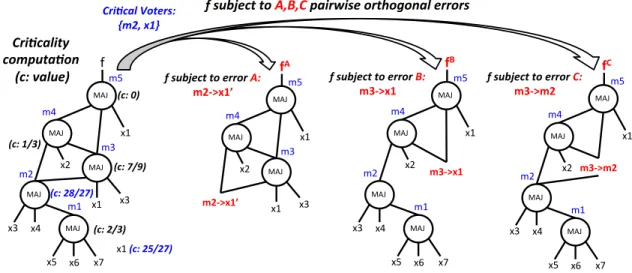
decision, i.e., influencing a Boolean function most. We call such nodescritical votersof a MIG. Critical voters can also be primary input themselves. To determine the critical voters, we rank MIG nodes based on a criticalitymetric. Thecriticality computation goes as follows. Consider a MIG node m. We label all MIG nodes whose computation depends on m. For all such nodes, we calculate the impact ofm by propagating a unit weight value from m outputs up to the root with an attenuation factor of 1/3 each time a majority node is encountered. We finally sum up all the values obtained and call this result criticality of m. Intuitively, MIG nodes with the highestcriticalityare critical voters.

For the sake of clarity, we give an example of criticality computation in Fig. 3. Node m5 has criticality of 0, since it is the root and does not propagate to any node. Node m4

has criticality of 1/3 (a unit weight propagated to m5 and attenuated by 1/3). Node m3 has criticality of 1/3 (m4) + (1/3+1)/3 (direct andm4contribution tom5) which sums up to 7/9. Node m2 has criticality of 1/3 (m3) + 4/9 (m4) + 7/27 (m5) which sums up to 28/27. Node m1 hascriticality 1/3 +criticalityofm2attenuated by factor 3 which sums up to about 2/3. Among the inputs, onlyx1has a notablecriticality being 1/3 (m3) + 1/9 (m4) + (1/3+1/9+1)/3 (m5) which sums up to 25/27. Here the two elements with highestcriticalityare m2 andx1.

We first determine two critical votersa andb and a set of MIG nodes fed directly by bothaand b, say {c1, c2, ..., cn}.

In this context, an advantageous triplet of orthogonal errors is: A: a = b0, B: c1 = a, c2 = a, ..., cn = a and C: c1 =

b, c2 = b, ..., cn = b. Consider again the example in Fig. 3.

There, the critical voters are a = m2 and b = x1, while c1=m3. Thus, the pairwiseorthogonalerrors are m2 =x10

(A),m3 =x1(B) andm3 =m2(C), as shown in Fig. 3. The actualorthogonality of A,B andC type of errors is proved in the following theorem.

Theorem 5.1: Letaandbbe two critical voters in a MIG. Let{c1, c2, ..., cn}be the set of MIG nodes fed by bothaand bin the same polarity. Then, the following errors are pairwise orthogonal: A: a=b0, B: c1=a, c2=a, ..., cn =a andC: c1=b, c2=b, ..., cn=b.

Proof: Starting from a MIG w, we build the three erroneous versions wA_{, w}B _and _wC _{as described above. We}

show thatorthogonalityholds for all 3 pairs.Pair (wA_{, w}B_):

We need to show that(wA_⊕_w₎_·₍_wB_⊕_w_{) = 0}_{. The element} wA _⊕_w _implies _a ₌ _b_{, being the difference between the}

original and the erroneous one with a = b0 (a 6= b). The element wB _⊕_w _implies _c

i 6= a (ci = a0), being the

difference between the original and the erroneous one with ci = a. However, if a = b then ci cannot be a0 because ci = M(a, b, x) = M(a, a, x) = a 6= a0 by construction.

Thus, the two elements cannot be true at the same time, making(wA_⊕_w₎_·₍_wB_⊕_w_{) = 0}_._{Pair (w}A_{, w}C_):_{This case}

is analogous to the previous one. Pair (wB_{, w}C_): _{We need}

to show that(wB_⊕_w₎_·₍_wC_⊕_w_{) = 0}_{. As we deduced before,}

the element wB_⊕_w _implies_c

i 6=a (ci =a0). Similarly, the

element wC_⊕_w _implies _c

i 6=b (ci =b0). By the transitive property of equality and congruence in the Boolean domain ci 6=a and ci 6= b implies a =b. However, if a =b, then ci = M(a, b, x) = M(a, a, x) = M(b, b, x) = a =b which

(9)

Cri$cal(Voters:(( {m2,(x1}( MAJ$ fB_# $ MAJ$ MAJ$ x1$ x2$ x4$ x3$ MAJ$ x7$ x6$ x5$ m1$ m2$ m3&>x1# m4$ m5$ MAJ$ fC_# MAJ$ MAJ$ x1$ x2$ x4$ x3$ MAJ$ x7$ x6$ x5$ m1$ m2$ m3&>m2# m4$ m5$ MAJ$ fA_# MAJ$ MAJ$ x1$ x2$ x3$ x1$ m2&>x1’# m3$ m4$ m5$ MAJ$ f$ MAJ$ MAJ$ MAJ$ x1$ x2$ x3$ x1$ x4$ x3$ MAJ$ x7$ x6$ x5$ m1$$ m2$$ m3# m4# m5# x1$(c:(25/27)( (c:(0)( (c:(7/9)( (c:(1/3)( (c:(28/27)( (c:(2/3)( Cri$cality(( computa$on(

((c:(value)( f(subject(to(error(A:( m2&>x1’#

f(subject(to(error(B:(

m3&>x1# f(subject(to(error(m3&>m2# C:(

f(subject(to(A,B,C(pairwise(orthogonal(errors#

Fig. 3: Example ofcriticalitycomputation andorthogonalerrors. true simultaneously, making(wB_⊕_w₎_·₍_wC_⊕_w_{) = 0}_.

Even though focusing on critical voters is typically a good strategy for safe error insertion in MIGs, sometimes other techniques can be also convenient. In the following, we present one of these alternative techniques.

2) Input Partitioning Method: As a complement to critical voters method, we propose a different way to derive advanta-geous triplets of orthogonal errors in MIGs. In this case, we focus on the inputs rather than looking for internal MIG nodes. In particular, we search for inputs leading to advantageous simplifications when erroneous. Analogously to thecriticality metric in critical voters, we use here a decision metric, called dictatorship[43], to select the most profitable inputs for logic error insertion. The dictatorship is the ratio of input patterns over the total (2n) for which the output assumes the same value as the selected input, in a chosen polarity [43]. For example, in the function f = (a+b)·c, the inputsa andbhave equal dictatorship of 5/8 while input c has an higher dictatorship of 7/8. The inputs with the highest dictatorship are the ones where we want to insert logic errors. Indeed, they have the largest influence on the circuit functionality and its structure. Exact computation of the dictatorship requires exhaustive simulation of an MIG structure, which is not feasible for practical reasons. Heuristic approaches to estimatedictatorship involve partial random simulation and graph techniques [43]. After exact or heuristic computation of the dictatorship, we select a subset of the primary inputs with highestdictatorship. Next, for each selected input, we determine a condition that causes an error. We require these errors to beorthogonal. Since we operate directly on the primary inputs, we already divide the Boolean space into disjoint subsets that are orthogonal. Because we need at least three errors, we need to consider at least three inputs to be made erroneous, say x, y and z. A possible partition is the following: {x 6= y, x = y = z, x = y = z0}. The corresponding errors are A: x = y for {x6=y},B: z =y0 when x=y for {x= y =z} andC: z=ywhenx=yfor{x=y=z0}. We formally proveA, B andC orthogonality hereafter.

Theorem 5.2: Consider the input split {x6=y,x=y =z, x=y =z0} in a MIG. Three errors A, B andC selectively affecting one subset but not the others are pairwiseorthogonal. Proof: To prove the theorem it is sufficient to show that

the split {x 6= y, x = y = z, x = y = z0_} _{is actually a}

partition of the whole Boolean space, i.e., a union of disjoint (non-overlapping) subsets. It is an easy exercise to enumerate all the eight possible {x, y, z} input patterns and associate with each of them the corresponding {x 6= y, x = y = z, x=y=z0}subset. By doing so, one can see that no{x, y, z} pattern is associated with more than one sub-set, meaning that all subsets are disjoint. Moreover, all together, they form the whole Boolean space.

For the sake of clarity, we report an illustrative exam-ple on the input partitioning method. The function is f =

M(x, M(x, y0, z), M(x0, y, z)). The input split is {x 6= y, x =y = z, x= y = z0} which is affected by errors A, B andC, respectively. The first errorA imposesx=y leading tofA₌_M₍_{x, M}₍_{y, y}0_{, z}₎_{, M}₍_x0_{, x, z}₎₎_{which can be further}

simplified into fA = M(x, z, z) = z by Ω.M. The second errorB imposesz=y0 when x=y. This is the case for the bottom level majority operators M(x, y0, z) and M(x0, y, z)

which are transparent whenx=y. Therefore, errorBleads to fB = M(x, M(x, y0, y0), M(x0, y, y0)) which can be further simplified into fB ₌ _M₍_{x, y}0_{, x}0_{) =} _y0 _by _Ω_.M_{. The third}

error C imposes z = y when x = y holds. Analogously to errorB, errorCleads tofC₌_M₍_{x, M}₍_{x, y}0_{, y}₎_{, M}₍_x0_{, y, y}₎₎

which can be further simplified intofC =M(x, x, y) =xby

Ω.M. A top majority node finally merges the three functions into f = M(fA, fB, fC) = M(z, y0, x) which correctly represents the objective function but has 2 fewer nodes and 1 level less than the original representation.

B. Depth-Oriented MIG Boolean Optimization

The most intuitive way to exploit safe error insertion in MIGs is to reduce the number of levels. This is because the initial overhead in w = M(wA_{, w}B_{, w}C₎_{, where} _w _is

the initial MIG and wA_{, w}B_{, w}C _{are the three erroneous}

versions, is just one additional level. This extra level is usually amply recovered during simplification and optimization of MIG erroneous branches. For depth-optimization purposes, the critical voters method introduced in Section III-C enables very good results. The reason is the following. Critical voters appear along the critical path more than once. Thus, the possibility to insert simplifying errors on critical voters directly enables a strong reduction in the maximum number of levels.

(10)

Some-MAJ$ f$ MAJ$ MAJ$ MAJ$ x1$ x2$ x3$ x1$ x4$ x3$ MAJ$ x7$ x6$ x5$ m1$ m2$ m3$ m4$ m5$ MAJ$ MAJ$ MAJ$ x1$ x2$ x4$ x3$ MAJ$ x7$ x6$ x5$ m1$ m2$ m4$ m5$ fm3/m2$ MAJ$ MAJ$ x1$ x4$ x3$ MAJ$ x7$ x6$ x5$ m1$ m2$ m5$ fm3/m2$ MAJ$ x4$ x3$ MAJ$ x7$ x6$ x5$ m1$ m2$ fm3/m2$ Ω.M$ Ω.M$ MAJ$ fm2/x1’_$_fm3/m2$ _fm3/x1$ f$ Cri$cal(Voters:(( {m2,(x1}( MAJ$ MAJ$ MAJ$ x1$ x2$ x4$ x3$ MAJ$ x7$ x6$ x5$ m1$ m2$ m4$ m5$ fm3/x1$ x1$ fm3/x1$ x1$ Ω.M$ MAJ$ MAJ$ MAJ$ x1$ x2$ x3$ x1$ m3$ m4$ m5$ fm2/x1’_$ x1$ MAJ$ MAJ$ x1$ x2$ m4$ m5$ fm2/x1’_$ x1$ x3$ MAJ$ MAJ$ x1$ x2$ m4$ m5$ fm2/x1’_$ x1$ x3$ fm2/x1’_$ x3$ Ω.M$ Ω.A$ Ω.M$

f

m3/x1

_'

f

m2/x1’

_'

f

m3/m2

_'

Cri$cal(path( Depth:(5( Size:(5( Depth:(2( Size:(3( Depth(gain:(60%( Size(gain:(40%( Cri$cal(path( Final(MIG( Original(MIG( Last(Gasp( Alg.(Opt.( Alg.(Opt.( Alg.(Opt.( Top(MAJ( Masking(Node( MAJ$ f$ x1$ x3$ _MAJ$ x4$ x3$ MAJ$ x7$ x6$ x5$ MAJ$ f$ x3$ MAJ$ x4$ x3$ MAJ$ x7$ x6$ x5$ x1$ Ω.A$

Fig. 4: MIG Boolean depth-optimization example based on critical voters errors insertion. Final depth reduction: 60%. times, using an actual MIG root for error insertion requires an

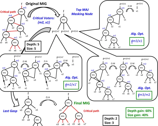
unpractical size overhead. In these cases, we bound the critical voters search to sub-MIGs partitioned on a depth criticality basis. Once the critical voters and a proper error insertion root have been identified, three erroneous sub-MIG versions are generated as explained in Section III-C. On these sub-MIGs, we want to reduce the logic height. We do so by running algebraic MIG optimization on them (Alg. 2). Note that, in principle, also MIG Boolean methods can be re-used. This would correspond to a recursive Boolean optimization. However, it turned out during experimentation that algebraic optimizations already produce satisfactority results at the local level. Thus, it makes more sense to apply Boolean techniques iteratively on the whole MIG structure rather than recursively on the same logic portion. At the end of the optimization of erroneous branches, the new MIG-roots must be given in input to a top majority voting node. This re-establishes the functional correctness. A last gasp of MIG algebraic optimization is applied at this point, to take advantage of the simplification opportunities arosen from the integration of erroneous branches. This Boolean optimization strategy is summarized in Alg. 3.

We comment on the MIG Boolean depth optimization with a simple example, reported in Fig. 4. First, the critical voters are searched and identified, being in this example the inputx1

and the nodem2(from Fig. 3). The proper error insertion root in this small example is the MIG root itself. So, three different versions of the root f are generated with errors fm2/x10_,

Algorithm 3 MIG Boolean Depth-Optimization Pseudocode INPUT:MIGα OUTPUT:Optimized MIGα.

for(cycles=0; cycles<effort; cycles++) do

{a, b}=search critical voters(α);// Critical votersa, bsearched

c=size bounded root(α, a, b);// Proper error insertion root

xn₁=common parents(α, a, b);// Nodes fed by bothaandb

cA=cb/a0;// First erroneous branch

cB_=cxn₁/a_;_{// Second erroneous branch}

cC_=cxn

1/b_;_{// Third erroneous branch}

MIG-depth Alg Opt(cA_);_{// Reduce the erroneous branch height}

MIG-depth Alg Opt(cB_);

// Reduce the erroneous branch height

MIG-depth Alg Opt(cC_);_{// Reduce the erroneous branch height} c=M(cA_{, c}B_{, c}C₎_;

// Link the erroneous branches

MIG-depth Alg Opt(c); // Last Gasp

ifdepth(c) is not reducedthen revert to previous MIG state; end if

end for

fm3/m2 and fm3/x1. Each erroneous branch is handled by fast algebraic optimization to reduce its depth. The detailed algebraic optimization steps involved are shown in Fig. 4. The most common operation is Ω.M that directly simplifies the introduced errors. The optimized erroneous branches are then linked together by a top fault-masking majority node. A last gasp of algebraic optimization on the final MIG structure further optimizes its depth. In summary, our MIG Boolean optimization techniques attains a depth reduction of 60%.

(11)

C. Size-Oriented MIG Boolean Optimization

Safe error insertion in MIGs can be used for size reduc-tion. In this case, the branch triplication overhead in w =

M(wA, wB, wC) imposes tight simplification requirements. One way to handle this situation is to enforce stricter selection metrics on critical voters. However, the benefits deriving from this approach are limited. A better solution is to change the type of error inserted and use the input partitioning method. Indeed, the input partitioning methodcan focus on the most influent inputs of a MIG, and introduces selective simplifica-tion on them. The resulting Boolean optimizasimplifica-tion procedure is similar to Alg. 2 but with depth techniques replaced by size techniques, and critical voter search replaced by input partitioning methods.

VI. EXPERIMENTALRESULTS

In this section, we test the performance of our MIG opti-mization techniques on academic and industrial benchmarks. We run logic optimization experiments (comparing logic net-works) and complete design experiments (consisting of logic synthesis and physical design) on commercial ASIC and FPGA flows. Finally, we give our vision on nanotechnology design via MIGs.

A. Methodology

We developed a majority-logic manipulation package, called MIGhty, consisting of about 8k lines of C code. It embeds various optimization commands based on the theory presented so far. In this work, we use a particular MIGhtyoptimization strategy targeting strong depth reduction interleaved with size recovery phases. The top-level optimization script is depicted by Alg. 4. This technique starts by reducing the depth by Algorithm 4 Top-Level MIG-optimization Script

INPUT: MIGα. OUTPUT:Optimized MIG α. MIG-depth Alg Opt(α);// small size overhead

MIG-reshaping(α);// reshuffling

MIG-size Alg Opt(α);// no depth overhead

MIG-depth Bool Opt(α);// pronounced size overhead

MIG-depth Alg Opt(α);// small size overhead

MIG-size Bool Opt(α);// small depth overhead

MIG-depth Alg Opt(α);// small size overhead

algebraic methods implying a small size overhead. After a fast reshaping step, it decreases the size of the MIG by level-bounded size reduction. At this point, Boolean MIG depth optimization is invoked to significantly reduce the number of levels at the price of a temporary MIG size inflation. Further level reduction opportunities are exploited in an algebraic depth reduction step. Then, size recovery is achieved by Boolean intertwined with algebraic size reduction. A small depth overhead is possible in this phase due to the size reduc-tion. Finally, a last gasp of algebraic depth optimization further compacts the MIG followed by level-bounded algebraic size reduction. All optimization steps have a runtime complexity linear w.r.t. the MIG size, i.e., are imposed to consider each node at least once.

The script in Alg. 4 is a composite optimization strategy, similarly to the class of resynscripts in ABC [2].

MIGhty reads files in Verilog or AIGER format and writes back a Verilog description of the optimized MIG. In order to simplify successive mapping steps, MIGhty reduces majority functions into AND/ORs if no size/depth overhead is implied. Thus, only the essential majority functions are written. Also, the number of inversions is minimized byΩ.I before writing. We consider IWLS’05 Open Cores benchmarks and larger arithmetic HDL benchmarks. As a case study, we also consider various adder circuits. All the Verilog files deriving from our experiments can be downloaded at [44], for the sake of reproducibility. In all benchmarks, we assumed the input signals to be available at time 0. In total, we optimized about half a million equivalent gates over 31 benchmarks.

For the pure logic optimization experiments, we use as reference tool the ABC academic synthesizer [2], with the delay oriented scriptif−g;iresyn. The initialif−g optimiza-tion strongly reduces the AIG depth by using SOP-balancing [51]. The latter iresyn optimization performs fast rewriting passes on the AIG, reducing mostly the number of nodes but potentially also the number of levels.

We chose the AIG script if−g;iresyn because its opti-mization rationale is close to our MIG optiopti-mization strategy and the respective runtimes are comparable. Note that ABC offers many other optimization scripts. Some of them may give better results under determinate conditions (benchmark type, size etc.). As the purpose of this work is primarily to assess the potential of MIG optimization w.r.t. to analogous AIG optimization, we neglect considerations and comparisons related to other ABC commands.

While comparing size and depth of MIGsvs.AIGs already gives some good intuition on a data structure and optimization effectiveness, we aim at providing results on even grounds. For this reason, we map both AIG-optimized and MIG-optimized circuits onto LUT6. We perform LUT mapping using the established ABC scriptdch−f;if −m−K 6.

For the complete design experiments, we consider a 22-nm (28-nm) commercial ASIC (FPGA) flow suite. The commer-cial flow consists of a logic synthesis step followed by place & route. In this case, we use the MIG-optimized Verilog file as input to the commercial tools in place of the original Verilog file. In other words, theMIGhty package operates as a front-end to the flows. Indeed, the efficiency of MIG-optimization helps the commercial tool to design better circuits. With the final circuit speed being our main design goal, we use an ultra-high delay effort scriptin the commercial tools.

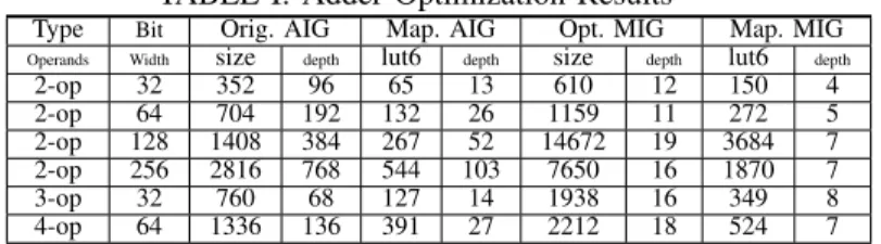
TABLE I: Adder Optimization Results

Type Bit Orig. AIG Map. AIG Opt. MIG Map. MIG

Operands Width size depth lut6 depth size depth lut6 depth

2-op 32 352 96 65 13 610 12 150 4 2-op 64 704 192 132 26 1159 11 272 5 2-op 128 1408 384 267 52 14672 19 3684 7 2-op 256 2816 768 544 103 7650 16 1870 7 3-op 32 760 68 127 14 1938 16 349 8 4-op 64 1336 136 391 27 2212 18 524 7 B. Optimization Case Study: Adders

We first test the MIG optimization capabilities for adders, that are known hard-to-optimize circuits [52]. Results for more general benchmarks are given in the next subsection. Table I shows the adder results. Our optimized MIG adders have 4 to

(12)

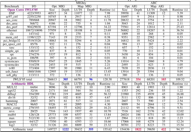
TABLE II: MIG Logic Optimization and LUT-6 Mapping Results

MIGhty ABC

Benchmark I/O Opt. MIG Map. MIG Opt. AIG Map. AIG

Open Cores IWLS’05 Size Depth LUT6 Depth Runtime (s) Size Depth LUT6 Depth Runtime (s) DSP 4223/3953 40517 34 11077 11 7.98 39958 41 11309 12 5.39 ac97 ctrl 2255/2250 10745 8 2917 3 6.52 10497 9 2914 3 8.98 aes core 789/668 20947 18 3902 4 11.78 20632 19 3754 5 8.22 des area 368/72 4186 22 735 6 1.04 5043 24 1012 7 2.11 des perf 9042/9038 67194 15 12796 3 34.22 75561 15 12814 3 25.43 ethernet 10672/10696 57959 15 18108 6 23.69 56882 22 18267 6 36.54 i2c 147/142 971 8 270 3 0.11 1009 10 268 4 0.05 mem ctrl 1198/1225 7143 19 2333 7 0.38 9351 22 2582 7 0.33 pci bridge32 3519/3528 18063 16 5294 6 3.28 16812 18 5424 7 2.22 pci spoci ctrl 85/76 932 11 276 4 0.04 994 13 287 4 0.02 sasc 133/132 621 6 152 2 0.11 657 7 152 2 0.03 simple spi 148/147 837 8 206 3 0.05 770 10 211 3 0.01 spi 274/276 3337 19 812 6 3.71 3430 24 854 7 2.28 ss pcm 106/98 397 6 104 2 0.01 381 6 104 2 0.01 systemcaes 930/819 9547 25 1845 7 5.26 11014 31 2060 8 4.79 systemcdes 314/258 2453 19 515 5 2.21 2495 21 623 5 1.05 tv80 373/404 7397 30 1980 11 6.43 7838 35 2036 11 2.97 usb funct 1860/1846 12995 19 3333 5 13.45 13914 20 3394 5 9.04 usb phy 113/111 372 7 136 2 0.11 380 7 136 2 0.05 IWLS’05 total 266613 305 66791 96 120.38 277618 354 68201 103 109.52

Arithmetic HDL Size Depth LUT6 Depth Runtime (s) Size Depth LUT6 Depth Runtime (s)

MUL32 64/64 9096 36 1852 10 2.90 8903 40 1993 11 1.90 sqrt32 32/16 2171 164 544 54 1.02 1353 292 236 55 1.22 diffeq1 354/289 17281 219 4685 45 56.32 21980 235 4939 45 16.88 div16 32/32 4374 102 818 37 4.67 5111 132 806 38 2.44 hamming 200/7 2071 61 517 14 2.01 2607 73 590 17 2.54 MAC32 96/65 9326 41 2095 11 4.30 9099 54 2044 12 7.76 metric comp 279/193 18493 77 6202 29 16.21 21112 95 6796 31 9.51 revx 20/25 7516 143 1937 40 10.70 7516 162 2176 42 12.02 mul64 128/128 25773 109 6557 31 13.84 26024 186 6751 43 10.09 max 512/130 4210 29 1023 12 1.67 2964 113 818 20 2.23 square 64/127 17550 40 4393 13 18.66 17066 168 4278 35 12.24 log2 32/32 31326 201 8809 59 23.32 30701 272 8223 73 15.54 Arithmetic total 149727 1222 39432 355 155.62 154436 1822 39650 422 94.37

48× smaller depth than the original AIGs. In all cases, the optimized MIG structure resembles a carry-look ahead design which is known to be the most depth-efficient for adders. Considering LUT mapped results, MIG-optimization enables significantly less deep circuits, having 1.75 to 14× smaller depth than LUT6 circuits mapped from the original AIGs. C. General Optimization Results

Table II shows general results forMIGhtylogic optimization and LUT-6 mapping. For the IWLS’05 and HDL arithmetic benchmarks, we see a total improvement in all size, depth and switching activity metrics, w.r.t. to AIG optimized by ABC. The switching activity is computed by the ABC command ps -p. The same improvement trend holds also for LUT mapped circuits. Since logic depth was our main optimization target, we notice there the largest reduction.

Considering the IWLS’05 benchmarks, that are large but not deep,MIGhtyenables about 14% depth reduction. At the LUT-level, we see about 7% depth reduction. At the same time, the size and switching activity are reduced by about 4% and 2%, respectively. At the LUT-level, size and switching activity are reduced by about 2% and 1%, respectively.

Focusing on the arithmetic HDL benchmarks, we see a better depth reduction. Here, MIGhty enables about 33% depth reduction. At the LUT-level, it enables about 16% depth reduction. At the same time, MIGhty reduces size and switching activity by 4% and 0.1%. At the LUT-level, this corresponds to about 1% size reduction and practically the same switching activity.

The switching activity numbers are not reported in Table II for space reasons but can be reproduced using the ABC commandps -pon the files downloadable at [44].

Table II confirms that the runtime of our tool is similar with that ofif −g;iresynABC script.

All MIG output Verilog files passed formal verification tests (ABCcecand Synopsys Formality) with success.

D. ASIC Results

Table III shows the results for ASIC design (synthesis fol-lowed by place and route) at a commercial 22-nm technology node2_{. In total, we see that by using} _MIGhty _{as front-end}

to the ASIC design flow, we obtained better final circuits, in all relevant metrics including area, delay and power. For the delay, which was our critical design constraint, we observe an improvement of about 13%. This improvement is not as large as the one we saw at the logic optimization level because some of the gain got absorbed by the interconnect overhead during physical design. However, we still see a coherent trend: We got about 4% and 3% reductions in area and power.

E. FPGA Results

Table IV shows the results for FPGA design (synthesis followed by place and route) on a commercial 28-nm technol-ogy node3_{. By employing} _MIGhty _{as front-end to the FPGA}

design flow, we obtain better final circuits, in LUT count, delay and power metrics. For the delay, that was our critical design constraint, we observe an improvement of about 10%.